MISSING DATA IMPUTATION USING MACHINE LEARNING AND NATURAL LANGUAGE PROCESSING FOR CLINICAL DIAGNOSTIC CODES
Arkopal Choudhury
A dissertation submitted to the faculty of the University of North Carolina at Chapel Hill in partial fulfillment of the requirements for the degree of Doctor of Philosophy in
the Department of Biostatistics in the Gillings School of Global Public Health.
Chapel Hill 2020
Approved by: Michael R. Kosorok Feng-Chang Lin
Anna Kucharska-Newton John S. Preisser
ABSTRACT
Arkopal Choudhury: Missing Data Imputation Using Machine Learning and Natural Language Processing for Clinical Diagnostic Codes
(Under the direction of Michael R. Kosorok)
Imputation of missing data is a common application in supervised classification problems, where the feature matrix of the training dataset has various degrees of miss-ingness. Most of the former studies do not take into account the presence of the class label in the classification problem with missing data. A widely used solution to this problem is missing data imputation based on the lazy learning technique, k-Nearest Neighbor (KNN) approach. We work on a variant of this imputation algorithm using Gray’s distance and Mutual Information (MI), called Class-weighted Gray’s k-Nearest Neighbor (CGKNN) approach. Gray’s distance works well with heterogeneous mixed-type data with missing instances, and we weigh distance with mutual information (MI), a measure of feature relevance, between the features and the class label. This method performs better than traditional methods for classification problems with mixed data, as shown in simulations and applications on University of California, Irvine (UCI) Ma-chine Learning datasets (http://archive.ics.uci.edu/ml/index.php).
learning technique which captures complex interactions between mixed type data. We propose a proximity imputation and missForest type covariate imputation with random splits while building the forest. The performance of the imputation techniques used is compared to existing techniques in various simulation settings.
ACKNOWLEDGMENTS
It has been quite a journey over the last 6 years. When I got into this program, I never imagined graduating with so many experiences - I have really learnt a lot about myself as well as life in general. I would like to thank all the wonderful people who helped me shape this journey. For academic help, I would like to thank my advisor Dr. Michael Kosorok, my committee members Dr. Anna Kucharska Newton, who worked with me in the ARIC-based projects, Dr. John Preisser, who helped me write my first collaborative manuscript in UNC Chapel Hill, Dr. Haibo Zhou who taught me Linear Models and Dr. Feng-Chang Lin, who gave me valuable suggestions to improve my first paper. I would also like to thank Crystal, Phoebe and Sujatro for helping me with various programming tips and concepts throughout my PhD life. The members of the Kosorok lab, Sebastian, Daniel, Michael (Lawson), Sean, Duyeol, Ben, Hunyong, Nikki and John - you really helped me with your ideas and insights.
me by always being there to talk to or have fun. Thanks to all those who helped my party and liven up the college town experience. I would thank Jyotishka and Shalini (Choudhury) for the wonderful parties they organized, and I really missed those. It has been tough seeing most of you leave the Triangle area, and life hasn’t been the same over the last one year without you. I would also like to thank my friends in Raleigh, Moumita, Indranil, Salil, Arnab (Chakraborty), Suman (Majumdar), Rahul (Ghoshal), Rahul (Chakraborty), Dhrubajyoti, Tuhin and Sukanya - it was a pleasure playing Mafia, cricket and board games with you. I also had the pleasure hanging out with my friends from Durham, Aritra (Dasgupta), Debarati and Sneha.
TABLE OF CONTENTS
LIST OF TABLES . . . x
LIST OF FIGURES . . . xi
LIST OF ABBREVIATIONS . . . xii
CHAPTER 1: INTRODUCTION . . . 1
CHAPTER 2: MISSING DATA IMPUTATION FOR CLAS-SIFICATION PROBLEMS . . . 4
2.1 Introduction . . . 4
2.2 Methodology . . . 10
2.2.1 Formulation of the Problem . . . 10
2.2.2 k-Nearest Neighbors (KNN) Imputation Algorithm . . . 13
2.2.3 Mutual Information (MI) for Classification . . . 18
2.2.4 Grey Relational Analysis (GRA) based KNNI . . . 22
2.2.5 Transformation of the Data . . . 24
2.2.6 The Proposed Class-weighted Grey k-Nearest Neighbor (CGKNN) Algorithm . . . 24
2.2.7 Time Complexity of the Algorithm . . . 27
2.3 Simulation Studies . . . 27
2.3.1 Performance Measure . . . 30
2.3.2 Simulation Scenarios: . . . 30
2.4 Applications to UCI Machine Learning Repository Datasets . . . 35
CHAPTER 3: RANDOM FOREST IMPUTATION OF MISS-ING COVARIATES FOR LONGITUDINAL DATA
MODELS. . . 41
3.1 Introduction . . . 41
3.2 Methodology . . . 44
3.2.1 Formulation of the Problem . . . 44
3.2.2 Classification and Regression Trees (CART) . . . 46
3.2.3 Random Forests . . . 49
3.2.4 Random Forest Imputation . . . 50
3.3 Simulation Studies . . . 55
3.3.1 Missing Completely at Random (MCAR) . . . 57
3.3.2 Missing at Random (MAR) . . . 59
3.4 Discussion . . . 61
CHAPTER 4: NATURAL LANGUAGE PROCESSING FOR CLINICAL DIAGNOSTIC CODES . . . 62
4.1 Introduction . . . 62
4.2 Methodology . . . 64
4.2.1 Principal Components Analysis (PCA) . . . 64
4.2.2 Non-negative Matrix Factorization (NMF) with Gram Schmidt Orthogonalization . . . 65
4.3 Results . . . 68
4.4 Discussions . . . 74
LIST OF TABLES
2.1 RMSE Upon Convergence for the Toy Dataset . . . 32
2.2 Classification Accuracy (%) for the Toy Dataset . . . 33
2.3 RMSE Upon Convergence for the Toy MAR Dataset . . . 34
2.4 Classification Accuracy (%) for MAR Dataset . . . 35
2.5 Characteristics of the UCI Datasets Used for Data Analysis . . . 36
2.6 Comparison of RMSE of Iris Dataset . . . 37
2.7 Comparison of RMSE of Voting Dataset . . . 38
2.8 Comparison of RMSE of Hepatitis Dataset . . . 38
3.1 RMSE Upon Convergence for MCAR Fixed Effects Model . . . 58
3.2 RMSE Upon Convergence for MCAR Mixed Effects Model . . . 58
3.3 RMSE Upon Convergence for MAR Fixed Effects Model . . . 60
LIST OF FIGURES
2.1 3D Centers of Each Class Represented Without Noise Variables . . . . 31
2.2 Convergence of RMSE for Nearest Neighbors Algorithms at 10% MCAR 32 2.3 Convergence of RMSE for Nearest Neighbors Algorithms at 20% MAR 35 2.4 MI for the Sepal and Petal Lengths and Widths of Iris Dataset . . . 36
2.5 MI for Voting Dataset . . . 36
2.6 MI for Hepatitis Dataset . . . 37
2.7 Classification Accuracy for the Iris Dataset at (a) 5% (b) 10% and (c) 20% Rates of Missingness After Using NN Imputation . . . 38
3.1 RMSE for all the RF Algorithms at 20% MCAR . . . 58
3.2 RMSE for the 5 Algorithms at 20% MAR . . . 60
4.1 Dementia Patient Clustering Diagnostics . . . 69
4.2 Importance Measures of the Clusters . . . 70
4.3 Dendrogram of Important ICD-9 Codes in Dementia Patients With Hospitalizations Binned in 30 Day Groupings . . . 71
4.4 General Meaning of 3 Digit ICD-9 Codes . . . 71
4.5 Non-dementia Patient Clustering Diagnostics . . . 72
4.6 Importance Measures of the Clusters . . . 73
LIST OF ABBREVIATIONS
ARIC Atherosclerosis Risk in Communities CA Classification Accuracy
CART Classification and Regression Trees
CGKNN Classs-weighted Gray0s k-Nearest Neighbor
CMS Centers for Medicare & Medicaid Services EHR Electronic Health Records
EM Expectation Maximization FFS Fee-for-service
FWGKNN Feature-Weighted Gray0s KNN Imputation
GKNN Gray’s KNN Imputation GRA Gray Relational Analysis GRC Gray Relational Coefficient GRG Gray Relational Grade
HEOM Heterogeneous Euclidean Overlap Metric
ICD International Statistical Classification of Diseases IKNN Iterative k-Nearest Neighbors
KNN k-Nearest Neighbors Approach KNNI k-Nearest Neighbors Imputation LVQ Linear Vector Quantization MAR Missing At Random
MCAR Missing Completely At Random MI Mutual Information
MICE Multiple Imputation Using Chained Equations
NMF Non-negative Matrix Factorization NNI Nearest Neighbor Imputation
OOB Out of Bag
OTFI On The Fly Imputation
PCA Principal Components Analysis
PLANN Partial Logistic Artificial Neural Network PMM Predictive Mean Matching
RF Random Forest
RMSE Root Mean Squared Error
CHAPTER 1: INTRODUCTION
Missing data imputation has been an area of research for quite some time now. It had been been first worked on by Donald B. Rubin and Roderick J.A. Little since the 1970s (Rubin 1977, Little and Rubin 1987). However most of the applications has been on simple problems involving missing data where parametric models have been chosen as a method of imputation and in most cases, the data matrix had just a few missing values (the percentage of missingness was low). There has been relatively less work done on imputation (substitution by estimation) of missing values by
non-parametric methods like nearest neighbors, principal components, trees, etc. Non-parametric methods not only provide a flexible setting to apply the imputation methods on, but also are less biased than parametric methods in general. The only disadvantage suffered by non-parametric methods is the interpretability but it is counteracted by the other advantages and thus we prefer to look at these methods. The other setting where missing data imputation has not been worked out on is in relation to supervised classification problems when the outcome variable is known. Thus, we explore methods which will make use of the outcome variable while
imputing the values in the data matrix. In Chapter 2 of this manuscript we look into the Class-weighted Gray’s k-Nearest Neighbor (CGKNN) technique, which is a method of imputation for classification problems and works well for heterogeneous mixed type data too. This technique takes the class variable into account while imputing the data matrix in classification problem and this leads to better classification performance after imputation of the data matrix.
covariates are missing over different time periods, but the outcome is present at each time period. This is different from loss due to follow up as in the latter case, we would have the outcome missing as well for later time periods. An example of the former type of missingness would be the Atherosclerosis Risk in Communities (ARIC) Study Cohort where 15,792 participants who took part in the 1st visit back in
1987-1989 across 4 states in the USA (ARIC investigators 1989) and only 6,538 people returned for the 5th visit in 2011-2013. Out of the 9,254 individuals who did not come to the 5th visit, for a fraction of them, certain variables of interest could be ascertained through phone calls. Diabetes is one such outcome measured in the 5th visit for the 6,538 participants and some of the remaining 9,254 participants partially lost to follow up. However, a lot of covariate information is missing for participants whose diabetic status was ascertained through phone calls. There are not many studies in non-parametric missing data imputation techniques in longitudinal studies. We use a modified random forest technique using random splits (Ishwaran and Lu 2008) to impute the characteristics of the longitudinal dataset which has missingness due to follow-up or other reasons, followed by a prediction of the outcome using a suitable model. We are particularly interested in extending this idea from simulation settings to measuring the prevalence of diabetes among the ARIC participants and the factors which affect it, but due to the partial drop-outs, this measure would be biased. We use the Out-Of-Bag (OOB) error estimate of random forests to compute our imputation performance. The details of this is discussed in Chapter 3 which deals with variety of random forest imputation techniques in longitudinal datasets..
participants at the 5th visit and enrolled in continuous Medicare Fee-For-Service (FFS) Insurance in the 6 months prior to their visit, so that their hospitalization diagnostic (ICD-9) codes are available. Our aim is to distinguish between the hospitalization of patients who have been diagnosed with dementia from those without dementia at the 5th visit in the ARIC study, by clustering their
hospitalization diagnostic codes using text mining methods. The cognitive status diagnosis is taken from the 5th visit of the ARIC study. Our initial clustering of ICD codes using Non-negative Matrix Factorization (NMF) looks good when combined with Gram Schmidt Orthogonalization. We hope to get meaningful patterns of comorbidity preceding dementia using better text mining methods, to predict the onset of the disease. The details of this is discussed in Chapter 5, which deals with using natural language processing to cluster ICD codes in hospitalization records and distinguish between the comorbidity patterns of the patients with and without a dementia, before the official diagnosis of the disease.
The rest of this manuscript is organized as follows. A new method of missing data imputation for classification problems used nearest neighbors is introduced and shown in rigorous details in Chapter 2. A random forest based missing data
CHAPTER 2: MISSING DATA IMPUTATION FOR CLASSIFICATION PROBLEMS
2.1 Introduction
Many of the commonly used classification algorithms such as Classification and Regression Trees (CART) (Breiman et al. 1984) and Random Forests (Breiman 2001) do not have rigorous techniques for handling missing values in training data. Ignoring the datapoints with missing values and running the classification algorithm on
complete cases only leads to loss of vital information (Little and Rubin 2002). The occurrence of missing data is one of the biggest challenges for data scientists solving classification problems in real-world data (Duda et al. 2012). These datasets can come from any walk of life, ranging from medical data (Troyanskaya et al. 2001) and survey responses to equipment faults and limitations (Le Gruenwald 2005). The reason for missingness can be human error in inputting data, incorrect measurements,
non-response to surveys, etc. For example, an industrial database maintained by Honeywell, a company manufacturing and servicing complex equipment, has more than 50% missing data (Lakshminarayan et al. 1999) despite regulatory requirements for data collection. In wireless sensor networks, often due sensor faults, local
(Newman et al. 2008).
Classification problems are aimed at developing a classifier from training data so that a new test observation can be correctly classified into one of the groups/classes. The class membership is assumed to be known for each observation of the training set whereas the corresponding attributes/features may have some missing values. The test dataset consists of new observations having the corresponding features but no class labels. The goal of the classification problem is to assign class labels to the test set (Alpaydin 2009). In our problem setup, we assume that some of the features are missing at random (MAR) for the training as well as the test dataset. One approach to classification is ignoring the observations with missing values and building a classifier. This is only feasible when the missingness is insignificant, however, and it has been demonstrated that even with a 5% missingness, proper imputation increases the classification accuracy (Farhangfar et al. 2008). We focus on imputation of
missing values in the training as well as the test dataset so as to improve the overall performance of the classifier on the test data. Our proposed method takes into
account the class label during imputation of the training features, and this ensures an overall improvement in classification.
modeling of missing features and the relationship between them. Usually, incomplete datasets obtained from studies cannot be modeled accurately. The problem with single imputation techniques, in general, is they reduce the variance of the imputed dataset. These techniques are unable to calculate the standard error or confidence interval of the imputed values in the dataset. They are also very case-specific as they can meaningfully impute data only when the model is known or when the data is either numerical or discrete.
To solve the problems of single imputation, multiple imputation strategies generate several imputed datasets from which confidence intervals can be calculated. Multiple imputation is a process where several imputed datasets are created and the variance between these datasets reflect their uncertainty measures (Rubin 1977, Farhangfar et al. 2007). The earliest multiple imputation technique was the Expectation-Maximization (EM) Algorithm (Dempster et al. 1977). The EM Algorithm and its variants such as EM with bootstrapping (Honaker et al. 2011), assumes a parametric density function which fails miserably for features without a parametric density. A recent generalization of the EM Algorithm called Pattern Alternating Maximization with Lasso Penalty (MissPALasso) (Städler et al. 2014) has been applied to datasets with high dimensionality (p >> n), but also assuming
normality. Bayesian multiple imputation algorithms have been applied only to multivariate normal samples (Li 1988, Rubin and Schafer 1990).
Regression Imputation (Gelman and Hill 2006) is also a popular multiple
iteratively impute the missing values and also uses the class label of each sample as a predictor variable (Stein and Kowalczyk 2016). In Multiple Imputation using Chained Equations (MICE), the conditional distribution of each missing feature must be specified given the other features (Buuren and Oudshoorn 1999). It is assumed that the feature matrix has a full multivariate distribution from which the conditional distribution of each feature is derived. The full distribution need not be specified, as long as the distribution of each feature is stated, a feature called fully conditional specification (Buuren 2007). MICE can handle mixed types of data. It has options for predictive mean matching, linear regression, binary and polytomous logistic
regression, etc., and uses the Gibbs sampler to generate multiple imputations. However, for a given set of conditional distributions, a multivariate distribution may not exist (Buuren et al. 2006). The ideas of MICE and SRMI are combined in the MissForest approach (Stekhoven and Bühlmann 2011) which fits a random forest on the missing feature, using the other features as covariates and then predicts the missing values. This procedure is iterative and can handle mixed data, complex interactions, and high dimensions.
(Troyanskaya et al. 2001). The sequential KNN method was proposed using cluster-based imputation (Kim et al. 2004), followed by an iterative variant of the KNN imputation (IKNN) (Brás and Menezes 2007), both of which improves on KNNI. The Shelly Neighbors (SN) method improves the KNN rule by selecting only neighbors forming a shell around the missing datum, among the k closest neighbors (Zhang 2011). The first significant work in improving KNN imputation for
classification based problems uses a Mutual Information (MI)-weighted distance metric as a measure of closeness of a feature to the class label (García-Laencina et al. 2009). The method is called Mutual Information based k-Nearest Neighbor
(MI-KNN) Imputation. However, the distance metric used is Euclidean distance, which does not perform well with mixed-type data (Huang and Lee 2006).
Alternatively, Grey Relational Analysis is shown to be more appropriate for capturing proximity between two instances with mixed data as well as missingness. Based on this, a Grey KNN (GKNN) imputation approach was built based on Grey distance instead of Euclidean distance and it was shown to outperform traditional KNN imputation techniques (Huang and Lee 2004, Zhang 2012). This grey distance-based KNN imputation is weighted by mutual information between features (measure of inter-feature relevance) and shown to outperform IKNN, GKNN and Fuzzyk-Means Imputation (FKMI) (Li et al. 2004) in most settings, and is called the Feature
Weighted Grey k-Nearest Neighbor (FWGKNN) method (Pan et al. 2015). However, this method does not take into account each feature’s association with the class label, which is crucial when dealing with classification problems. The FWGKNN method also assumes inter-dependency of features.
instances, and then find thek-Nearest Neighbors of an instance with missing values. Using k-Nearest Neighbors, the missing value is imputed according to the weighted Grey distance. Our contributions can be summarized as follows:
1. We use a combination of Mutual Information between each feature and the classifier variable Y to weigh the Grey distance between instances in the feature matrix X. This metric is suited for tuning out any unnecessary features for classification and then finding the nearest neighbors relevant for imputation. 2. We solve an imputation problem with no underlying assumptions on the
structure of the feature matrixX except that the data is missing completely at random (MCAR) or missing at random (MAR). Our method (CGKNN) is non-parametric in nature and does not assume any dependence between the individual features. This performs well even when the features are independent of each other.
3. The proposed CGKNN imputation method is suited well for classification problems where the training as well as the test datasets have missing values. The feature matrix can be mixed-type, i.e., have categorical and numeric data. Our method is suitable for mixed-data classification problems faced with missing values. Moreover, our problem approach takes much less time to initialize than the most similar alternative method, Feature Weighted Grey k-Nearest Neighbor (FWGKNN).
The remainder of this paper is organized as follows. In Section 2, we review the KNN imputation techniques used in previous work and then provide a detailed
evaluate our imputation method (CGKNN) in different simulation settings with classification where we artificially introduce missingness. We compare it with standard multiple imputation algorithms MICE and MissForest as well as the
previous KNN based algorithms, Iterative KNNI (IKNN), Mutual Information based KNNI (MI-KNN), Grey KNNI (GKNN) and Feature-Weighted Grey KNNI
(FWGKNN). In section 4, we demonstrate how our algorithm performs with
classification tasks involving 3 UCI Machine Learning Repository datasets. We also check for improvement of classification accuracy after imputation of the missing data. Our method gives the best classification performance out of all evaluated methods. We conclude with a discussion and scope for future work in section 5.
2.2 Methodology
In this section, we pose the missing data problem which is encountered in classification tasks. We introduce the nearest neighbor (NN) approach and the previous works done on implementing variations on the KNN imputation approach. This is followed by the concepts of mutual information (MI) and grey relational analysis (GRA) used by our method of Class-weighted Greyk-Nearest Neighbor (CGKNN) imputation approach (Choudhury and Kosorok 2020). We then formalize our imputation algorithm and calculate its time complexity.
2.2.1 Formulation of the Problem
datasetX. In practice, we obtain a random sample of size n of incomplete data associated with a population(X, Y, D), called the training data (Hastie et al. 2009) used to train the classifier
D ={(Xi, Yi, Di)}ni=1, (2.1)
where all the class labels in {Yi}ni=1 are observed, Xi = (Xij)pj=1 = (Xi1, ..., Xip) represents the pfeatures of the i-th observation along with indicator variables Di = (Dij)pj=1 such that
Dij =
0, Xij is missing 1, otherwise.
(2.2)
Without loss of generality, we can assume for eachi, the observation Xi = (Xij)pj=1 contains p0 categorical features for j ∈ {1,2, ..., p0} and p1 continuous features for j ∈ {p0+ 1, ..., p0+p1} such thatp0+p1 =p. Let the j-th categorical feature contain kj different values and the j-th continuous variable representing the (p0+j)-th
feature ofXi, indexed by j ∈ {1, ..., p1}take values from a continuous set Cj ⊂R. For each of the categorical features, we can map thekj different values to the firstkj natural numbers, such that Xi ∈ {1, ..., k1} ×...× {1, ..., kp0} ×C1×...×Cp1 ⊂Rp.
In this setting, we can assume that{(Xi, Yi)}ni=1 satisfy the model
Yi =g(Xi), i= 1,2, ..., n, (2.3)
whereg(.) is an unknown function mapping a p-dimensional number (belonging to a subspace of Rp) to a discrete set G representing the class labels and Yi ∈G. We assume thatG contains m values and thus the classification problem is based on m classes.
{(Xi, Yi)}ni=1 to estimate g(.), which is referred to as ‘training’ a classifierg(.)ˆ . Given a new set of ` observations, X0 ={Xi0}`i=1, called the test dataset (Hastie et al. 2009), the classifier predicts the corresponding class Y0 ={Yi0}`
i=1 using Yˆi0 = ˆg(Xi0). Note that the test dataset X0 can also contain missing values. Many classification
algorithms have been shown to perform better in terms of classification accuracy after imputing the missing values in the feature matrix X (Farhangfar et al. 2008, Luengo et al. 2012) and then training the classifier. In this paper, we propose a nearest neighbor based imputation algorithm which is used to impute the missing values in X and then train the classifierg(.)ˆ . The same algorithm can be extended to the test dataset and impute the missing values in X0.
In general, there are three different missing data mechanisms as defined in the statistical literature (Little and Rubin 2002):
1. Missing Completely at Random (MCAR): When the missingness of X does not depend on the missing or observed values of X. In other words, usingD is as defined in (3.2),
P(D|X) = P(D), for allX (2.4)
2. Missing at Random (MAR): When the missingness of X depends on the
observed values ofX but not on the missing values ofX. If we split the training datasetX into two parts, observed Xobs and missingXmis, then
P(D|X) = P(D|Xobs), for all Xmis (2.5)
estimates of the missing values.
P(D|X) = P(D|Xobs, Xmis) (2.6)
For our problem, we assume that the missing data mechanism ofX is either MCAR or MAR.
2.2.2 k-Nearest Neighbors (KNN) Imputation Algorithm
KNN is a widely used instance-based, lazy-learning algorithm (Wu et al. 2008). The basic assumption behind instance-based learning methods is that the instances of a dataset with missing values would lie “close” to other instances with similar
properties (Aha et al. 1991). The KNN approach has been extended to imputation of missing data in various datasets (Troyanskaya et al. 2001). KNN imputation
techniques work well when the distribution of the dataset is unknown. The basic algorithm works by calculating k nearest observations (out of the n−1possible observations) from a particular observation with missing values. The distances are calculated using pre-imputed values in each observation. After calculating thek closest neighbors, mean of the other observations is used for imputation of continuous features and mode is used for imputation of the categorical features. Note that we do not create any predictive model in KNN imputation since it is an instance-based learning algorithm. Observations with multiple missing values of different type (continuous or categorical) can be imputed by KNN imputation.
2.2.2.1 Distance Metric for Mixed Data
(HEOM) (Batista and Monard 2003), denoted as d(Xa, Xb), is defined as
d(Xa, Xb) =
v u u t p X j=1
dj(Xaj, Xbj)2 , (2.7)
dj(Xaj, Xbj) =
1, Daj ∗Dbj = 0 from (3.2) d0(Xaj, Xbj), Xj is categorical
dN(Xaj, Xbj), Xj is quantitative
(2.8)
d0(Xaj, Xbj) =
0, Xaj =Xbj
1, Xaj 6=Xbj
(2.9)
dN(Xaj, Xbj) = |Xaj−Xbj| max(X.j)−min(X.j)
, (2.10)
wheremax(X.j)means the maximum value of n observations of feature X.j and min(X.j) means the minimum value of X.j when it is quantitative. The distance ranges from 0 to1 and also takes the value 1, when either of the observations are missing.
2.2.2.2 KNN Imputation
Let us focus on the problem where the j-th input feature of Xi is missing (i.e., Dij = 0 from (2.2)) and has to be imputed. The distances from Xi to all other instances ({Xk}nk=1,k6=i) in the training set are computed using HEOM defined by (2.7)-(2.10), the k-nearest neighbors are chosen with least distances. Let
AXi ={a`}k`=1 represents the set of k-nearest neighbors ofXi arranged in increasing order of its distance as defined by (2.7)-(2.10). The k-closest cases are selected after instances with missing entries in the incomplete feature are imputed using mean or mode imputation, depending on the type of feature (Troyanskaya et al. 2001).
After choosing k-nearest neighbors, the missing value imputation is estimated from the feature values of AXi. For continuous variables, the imputed value (Xeij) is
e
Xij = (1/k)Pk
`=1a`j. The weighted version of this average is based Xi (Dudani 1976), such that
e
Xij =
Pk
`=1w` a`j k∗Pk
`=1w`
, w` = 1
d(Xi, a`)
2, (2.11)
wherew` denotes the corresponding weight of the `-th nearest neighbor a` and d(Xi, a`) is as defined in (2.7)-(2.10).
For categorical or discrete variables, we impute the mode of the j−th feature of {a`}k
`=1 toXije . This assumes all neighbors have the same importance in the
imputation stage (Troyanskaya et al. 2001). An improvement to this is assigning a weightw` to each a`, with closer neighbors having greater weights. Using an approach similar to a distance-weighted KNN classifier (Dudani 1976), a suitable choice ofw` is
w`(Xi) =
d(ak, Xi)−d(a`, Xi) d(ak, Xi)−d(a1, Xi)
, (2.12)
d(ak, Xi) = d(a1, Xi), that is, all the distances are equal. Otherwise, for k (>1) neighbors, 0≤w` ≤1. Suppose thej-th input feature X.j has V possible discrete values with nv being the number of samples inAXi whose j−th feature has value v, v = 1,2, ..., V. The weighted mode is chosen by the category v∗ calculated by the category with the maximum weight in AXi given by
v∗ = arg max v
( nv X
`=1
w`(Xi)
)
Algorithm 1 Iterative KNN (IKNN) Imputation (García-Laencina et al. 2009) Input: (X, Y, D) with X ⊂Rn×p containing missing entries and Y the class labels. Output: Imputed feature matrix Xe with no missing values.
Procedure:
1. Initialization: Given the training dataset X, the missing values ofp0 categor-ical features are imputed by mode imputation and the missing values of the p1 continuous features are imputed by mean imputation using the observed data. We call the initially imputed matrix Xe0.
2. Choosing k: We use this imputed matrix, Xe0, to calculate the optimum value
ofkusing 10-fold cross validation (Stone 1974) to minimize the misclassification rate of predicting the class labelsY. This is thek used for choosing the nearest neighbors.
3. Iterative Step: Consider the iteration number t (≥ 1). In the t-th iteration, the imputed matrixXet is obtained by imputing the missing continuous features
(with correspondingDij = 0) using (2.11) and missing categorical features using (2.12)-(2.13). This step is repeated until the stopping criteria is reached. 4. Stopping Criterion: We stop at thed-th iteration when a stopping criteria is
met. The stopping criteria we propose is
max i,j:Dij=0|Xe
d
ij −Xeijd−1|< , (2.14)
2.2.3 Mutual Information (MI) for Classification
We can see that the above imputation algorithm does not consider the class label Y while computing the k-nearest neighbors. We can solve this using an effective procedure where the neighborhood is selected by considering the input feature
relevance for classification (García-Laencina et al. 2009). This input feature relevance for classification is measured by calculating the Mutual Information (MI) between the feature X.j and the class variable Y.
2.2.3.1 Notion of MI
Suppose a discrete random variable X has a probability density function (pdf) given by p(x) =P(X =x) where x∈Support(X). The entropy of a random variable X is given by
H(X) =− X
x∈Supp(X)
p(x)log p(x), (2.15)
wherelog has base2 in information theory, with the unit of entropy being bits. Now consider two random variables,X and Y. The joint entropy of X and Y is defined as
H(X, Y) =−X
x∈X
X
y∈Y
p(x, y)log p(x, y), (2.16)
wherep(x, y) is the joint pdf of X and Y, both of them being discrete. The conditional entropy for the same pair of variables is given by
H(Y|X) = −X
x∈X
X
y∈Y
p(x, y)log p(y|x), (2.17)
For continuous random variables, the entropy ofX is defined by
H(X) = −
ˆ
x
p(x)log p(x)dx, (2.18)
and the joint and conditional entropy of continuous random variables X and Y is given by
H(X, Y) = −
ˆ
x
ˆ
y
p(x, y)log p(x, y)dy dx, (2.19) H(Y|X) = −
ˆ
x
ˆ
y
p(x, y)log p(y|x)dy dx, . (2.20)
Mutual information (MI) is based on entropy and it quantifies the uncertainty of X givenY. For discrete random variablesX and Y it is
I(X;Y) = X x∈X
X
y∈Y
p(x, y)log p(x, y)
p(x)p(y) , (2.21)
and for continuous random variables it is
I(X;Y) =
ˆ
x
ˆ
y
p(x, y)log p(x, y)
p(x)p(y) dx dy (2.22) The entropy and MI satisfy the following relationship
I(X;Y) =H(Y)−H(Y|X), (2.23)
which is the reduction of the uncertainty of Y when X is known (Kullback 1997) since it can be re-written as I(X;Y) =H(X) +H(Y)−H(X, Y). Compared to the
with MI being0 for two independent variables.
2.2.3.2 Computation of MI in Classification Problems
Consider the class label Y for an m-class classification problem and let the number of observations in they-th class be ny such thatn1+n2+...+nm =n, as mentioned in (2.1). In terms of classification problems, we are interested in finding the relevance of the j-th feature X.j with the class label Y, which is measured by their Mutual Information (MI) given by
I(X.j;Y) =H(Y)−H(Y|X.j), (2.24)
In this equation, we have to estimate H(Y) and H(Y.j) to get I(Xˆ .j;Y). Note that Y is always discrete and the entropy of class variableY can be computed using (2.15) as
ˆ
H(Y) = −
m
X
y=1 ˆ
p(y)log p(y),ˆ (2.25)
where we estimate p(y) by p(y) =ˆ ny/n. The estimation of H(Y|X.j) can be obtained from (2.17) when X.j is discrete and from (2.20) when X.j is continuous. For discrete feature variables, estimating the probability densities can be achieved by means of a histogram approximation (Kwak and Choi 2002). We can estimatep(x, y)ˆ and p(yˆ |x) by histogram approximation to get
ˆ
H(Y|X.j) = −
X
x∈Supp(X.j) m
X
y=1 ˆ
p(x, y)log p(yˆ |x), (2.26)
we need to estimate the conditional density of x.j at them classes represented byy and not the joint density. We can use a Parzen window estimation approach to estimate p(x.j)(Kwak and Choi 2002) given by
ˆ p(x.j) =
1 n
n
X
i=1
φ(x.j−xij, h), (2.27)
whereφ(.)is the window function and h is smoothing parameter. Rectangular and Gaussian functions are suitable window functions (Duda et al. 2012) and ifh is selected appropriately,p(xˆ .j) converges to p(x.j)(Kwak and Choi 2002). We can calculate p(x.j|y)using the Parzen window approach
ˆ
p(x.j|y) = 1 ny
X
i∈Iy
φ(x.j−xij, h), (2.28)
whereIy is the set of observations with class label y. Finally, we the use Bayes rule and (2.27)-(2.28) to estimate p(y|x.j) as
ˆ
p(y|x.j) = ˆ
p(x.j|y) ˆp(y) ˆ
p(x.j)
, (2.29)
and then estimateH(Y|X.j)from (2.20) by replacing the integral by summation over training observations and usingp(x, y) =p(x)p(y|x)to arrive at
b
H(Y|X.j) =−
X
x.j ˆ p(x.j)
ny
X
y=1 ˆ
p(y|x.j)log p(yˆ |x.j). (2.30)
(García-Laencina et al. 2009), such that
λj =
I(X.j;Y)
Pp
j0=1I(X.j0;Y)
, (2.31)
and then the distance between instances is calculated similar to (2.7):
dI(Xa, Xb) =
v u u t
p
X
j=1
λjdj(Xaj, Xbj)2, (2.32)
wheredj(Xaj, Xbj) is as defined in (2.8). Using this feature relevance weighted
distance, replacing dwith dI (from (2.32)) in (2.11)-(2.12), and following Algorithm 1, we obtain the MI-KNN imputation algorithm (García-Laencina et al. 2009).
2.2.4 Grey Relational Analysis (GRA) based KNNI
Grey System Theory (GST) has been developed to tackle systems with partially known and partially missing information (Deng 1982). The system was named grey since missing data is represented by black whereas known data is white, and this system contains both missing and known data. To obtain Grey-basedk-nearest neighbors, we used Grey Relational Analysis (GRA) in our algorithm which is calculating Grey Distance between two instances. Grey distance measures similarity of two random instances, which involves the Grey Relational Coefficient (GRC) and the Grey Relational Grade (GRG).
Consider the setup in (2.1) where the training dataset has n observations and p features. The Grey Relational Coefficient (GRC) between two instances/observation Xa and Xb, when thej-th feature is continuous and observed for both instances, is
GRC (Xaj, Xbj) =
∆min + ρ∆max
|Xaj−Xbj| + ρ∆max
where∆min = mincmink|Xak−Xck|,∆max= maxcmaxk|Xak−Xck|, ρ∈[0,1] (usually ρ= 0.5 is taken (Deng 1982)),b, c∈ {1,2, ..., n}, and, k, j ∈ {1,2, ..., p} and
for categorical featurej,GRC(Xaj, Xbj)is 1 if they have the same values, 0 otherwise. If either Xaj orXbj is missing, then GRC(Xaj, Xbj) is 0. The Grey Relational Gradient (GRG) between the instances is defined as:
GRG(Xa, Xb) = 1 p
p
X
j=1
GRC(Xaj, Xbj), (2.34)
wherea ∈ {1,2, ..., n}. We note that if GRG(Xa, Xb)is larger than GRG(Xa, Xc) then the difference betweenXa and Xb is less than the difference betweenXa and Xc, which is the opposite of the Heterogenous Euclidean Overlap Metric (HEOM) (2.7) defined in Section 2.2.2.1. The Grey Relational Gradient satisfies the following axioms which makes it a distance metric (Deng 1982):
1. Normality: The value of GRG(Xa, Xb) is between 0 and 1.
2. Dual Symmetry: Given only two observationsXa and Xb in the relational space, then GRG(Xa, Xb) = GRG(Xb, Xa).
3. Wholeness: If 3 or more observations are made in the relational space then GRG(Xa, Xb) is generally not equal to GRG(Xb, Xa) for any b.
4. Approachability: GRG(Xa, Xb) decreases as the difference between Xaj and Xbj increases, other values in (2.33) and (2.34) remaining constant.
GRA is generally preferred over metrics such as Heterogeneous Euclidean Overlap Metric (HEOM) for grey systems with missing data (Huang and Lee 2004). It gives us a normalized measuring function for both missing/available and
due to its wholeness over the entire relational space. So instead of d(Xa, Xb) in (2.7), if we use GRG(Xa, Xb)to select the k-nearest neighbors and then proceed with the KNN Imputation technique without using weights, then it becomes Grey KNN (GKNN) Imputation (Zhang 2012).
2.2.5 Transformation of the Data
Before we apply our version of the algorithm, we make some transformation of the continuous features contained in the training dataset, since we deal with a wide variety of features whose ranges vary vastly. For example, the range of marks in a 10 point exam would be less than the range of marks for a 100 point exam, and both these marks may be in the same training dataset. The distance metric and
subsequently the k-nearest neighbor would be biased unless the ranges of the continuous variables are normalized. In our algorithm, we transformed thej-th feature of observation Xi as
Xij0 = Xij −minaXaj maxaXaj−minaXaj
, (2.35)
wherea, i ∈ {1,2, ..., n} and j ∈ {1,2, ..., p}. Thus (2.35) ensures all the continous
variables are between 0 and 1. Note that the distance metric associated with categorical variables (Euclidean or Grey-based) lie within 0 and 1 as well.
2.2.6 The Proposed Class-weighted Grey k-Nearest Neighbor (CGKNN)
Algorithm
Xb as follows
GRG(Xa, Xb) = p
X
j=1
λj GRC(Xaj, Xbj). (2.36)
Since GRG(Xa, Xb) increases for closer neighbors unlike the other distance metrices, we used(Xa, Xb) = 1−GRG(Xa, Xb)in section 2.2.2.2 and then measure the distance between instances to choose thek-nearest neighbors,{a`}k`=1. From (2.11), we derive that the corresponding weights ofa` are
w` =
1
(1−GRG(Xi, a`))2
. (2.37)
Using these weights, we impute the continuous variables, and the new definition of d(Xa, Xb) in (2.12)-(2.13) is used to impute the categorical variables for our
Algorithm 2 Class-weighted Grey k-Nearest Neighbor (CGKNN) Imputation
Input: (X, Y, D)withX ⊂Rn×pcontaining missing entries andY themclass labels. Output: Imputed feature matrix Xe with no missing values.
Procedure:
1. Data pre-processing: First we transform the continuous features of X as suggested by 2.2.5 using (2.35) so that their ranges equal 1.
2. Initialization: We use the class labels inY to split X into {Xy}my=1. For each classy, given Xy, we pre-impute the missing values ofp
0 categorical features by mode imputation and the missing values of thep1 continuous features by mean imputation using the observed data in that class. We call it Xe0.
3. Mutual Information: Calculate the mutual information or the class weights λj of the attributes X.j using (2.24)-(2.31).
4. Choosing k: We use this imputed matrix, Xe0, to calculate the optimum value
of k using 10-fold cross validation by minimizing the misclassification rate. 5. Iterative Step: Consider iteration t(≥1) and class y. For each instance i in
the classy which has a missing value, calculate the GRG of that instance with all other instances of the classy. We find thek nearest neighbors{v`}k`=1. Using the weightsw` as described in (2.37), the imputed matrixXey,t is obtained with
d(Xa, Xb) = 1−GRG(Xa, Xb). This is repeated for each y until all missing values are imputed to obtain Xet = {Xey,t}my=1. If the stopping criterion is not
met, then the iteration on t continues.
6. Stopping Criterion: We stop at thed-th iteration when a stopping criteria is met. The stopping criteria we propose is
max i,j:Dij=0|Xe
d ij −Xed
−1 ij |<10
2.2.7 Time Complexity of the Algorithm
Consider the setup (2.1) with n observations, pfeatures and m classes. The time complexity for calculating the GRG in the biggest class containing (say) nj
observations is O(njp) and the average processing time for sorting theGRGs is O(njlognj). If we assume d iterations are taken for the algorithm to converge, then the algorithm has a complexity of O(d n2j plognj) to impute an nj ×p matrix. We do this for m classes and thus the time complexity for imputing ann×pmatrix is O(md n2
j plognj). Now, generally nj < n whenever m >1, which implies
lognj <logn, and nj∗m≥n since nj was the biggest class. This gives rise to the inequality
O(md n2j plognj)< O(d n2 plogn).
We initially calculate the Mutual Information of each attribute with the class
variable, which takesO(n p) time along with the imputation of the mean/mode which again takes O(p) time and choosing an optimumk which takes O(10∗n p r)time if we assumer values of k are tested using 10-fold cross-validation. So our total complexity becomes O(md n2
j plognj+np+p+ 10npr) which can be approximated toO(md n2
j plognj) if the value of nj is large compared to r. We note that this time complexity is similar to Grey KNNI (GKNN) and Feature-Weighted Grey KNNI (FWGKNN) but less than the O(d n2 plogn) complexity of Iterative KNNI (IKNN) and the Grey-Based Nearest Neighbor (GBNN) algorithm (Huang and Lee 2004).
2.3 Simulation Studies
We compare our method with 6 other well-established methods which are as follows:
• MICE (Multiple Imputation using Chained Equations): The MICE algorithm developed by Van Buuren and Oudshoorn (Buuren and Oudshoorn 1999) uses multiple imputation assuming that the columns ofX are Fully Conditionally Specified (FCS). We assume an imputation model for predicting missing values in each variable, based on the other variables. Generally, for continuous covariates, predictive mean matching is used for imputation. For categorical covariates, logistic regression is used for unordered covariates and proportional odds model for ordered covariates.
• MissForest: This is an iterative imputation method based on a random forest developed by Stekhoven and Buhlmann (Stekhoven and Bühlmann 2011). This non-parametric algorithm is basically similar to MICE except that each
predictive mode for imputation is random forest for both categorical and continuous variables. This method has an inbuilt imputation error estimate using the out-of-bag error estimate.
• Iterative k-Nearest Neighbor imputation (IKNN): In this method, k nearest instances are computed from the instance with a missing value, using Euclidean Distance as metric. Initial imputation is done using mean or mode imputation, followed by a calculation of the weighted mean or mode of the k nearest neighbors for each missing attribute. This process is done iteratively until the matrix is imputed with convergence between successive iteration steps. • Mutual Information based k-Nearest Neighbor imputation
Euclidean distance to measure the distance between instances, with the mutual information being the weights (García-Laencina et al. 2009). All imputed instances and all complete instances are considered to be known information for estimating missing values iteratively. The missing values are then imputed based on the weighted mean or mode of the nearest neighbors.
• Grey k-Nearest Neighbor imputation (GKNN): We use mean or mode imputation for an initial imputed matrix. This imputation method uses GRA to calculate the distance between instances and thus calculatek nearest neighbors for missing value imputation (Zhang 2012). The dataset is divided into separate parts based on the class label and imputation method is simultaneously
performed on each of them. The imputed values are again weighted mean or mode of thek nearest neighbors, with the distances and weights calculated by GRA.
• Feature Weighted Grey k-Nearest Neighbor (FWGKNN): This
2.3.1 Performance Measure
We measure the performance of each algorithm according to the following metrics:
• Root mean square error (RMSE): This measures how accurate or precise the imputation algorithm is as follows:
RM SE =
v u u t 1 np n X i=1 p X j=1
(Xij −X˜ij) 2
, (2.39)
whereei is the true value, ˜ei is the imputed value of the missing data, and m denotes the number of missing values.
• Classification accuracy (CA):We develop the imputation algorithm to assist in classification. After imputation of the dataset X, it is used in a suitable classification algorithm, whose accuracy is defined intuitively as follows:
CA= 1 n
n
X
i=1
I( ˜Yi =Yi), (2.40)
wheren is the number of observations of X,Y˜i is the predicted class value, Yi is the actual class value andI(.) is the indicator function.
2.3.2 Simulation Scenarios:
2.3.2.1 Missing Completely at Random (MCAR) Example
artificial problem. Two cubes belong to class 1, and they are centered on (0,0,0)and (−0.2,−0.4,0.4). The remaining two cubes are labeled with the class 2, being
centered on(−0.6,−0.6,0.5) and (0.4,−0.2,−0.2). In all the cubes, the width is equal to 0.20, and they are composed of 100 samples which are uniformly distributed inside the cube. In this problem, the MI values between the three attributes and the target class are computed: 0.69 for x1, 0.67 for x2, and 0.38 forx3.
Figure 2.1: 3D Centers of Each Class Represented Without Noise Variables
To this 3 dimensional, 2 class dataset we add 20 U[-1,1] variables. For these irrelevant variables, the MI between the feature and class variable is almost 0. We try to find out what happens when we add irrelevant attributes to classification. We insert 10% and 20% of missing data to x1, which is most relevant according to MI. The missingness of data inx1 is generated completely at random, which means it does not depend on the variable values in the matrixX.
discards the irrelevant features, and the selected neighborhood for missing data estimation tends to provide reliable values for solving the classification task. We provide a detailed analysis of how all the 6 algorithms performed in this simulation setting withn = 400, p= 23 and m= 2 classes in Table 2.1. Note that we used predictive mean matching as the imputation model for MICE. We also
Table 2.1: RMSE Upon Convergence for the Toy Dataset
Missing Rate MICE MissForest IKNN MI-KNN GKNN FWGKNN CGKNN 10% 0.2067 0.0915 0.2585 0.1023 0.2443 0.1155 0.0983
20% 0.3847 0.1943 0.3746 0.1852 0.3372 0.1803 0.1598
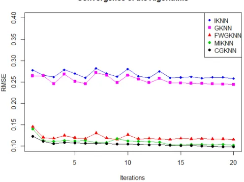
We empirically show the convergence of the nearest neighbor-type algorithms by plotting the RMSE against the iterations for the various algorithms in the case where 10% of the data is missing completely at random. The number of iterations plotted in Figure 3.2 is the maximum iterations taken by all of the algorithms to converge.
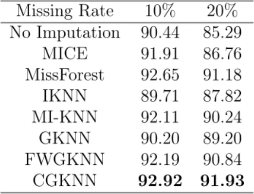
We also calculated the classification accuracy using the Naive Bayes method on the non-imputed and imputed datasets with 10% and 20% missing data, with the help of 10-fold cross validation process, using 80% of the data as training data. The
resulting improvement in accuracy for both the cases is highest for our CGKNN Algorithm, as shown in Table 2.2.
Table 2.2: Classification Accuracy (%) for the Toy Dataset Missing Rate 10% 20%
No Imputation 90.44 85.29
MICE 91.91 86.76
MissForest 92.65 91.18
IKNN 89.71 87.82
MI-KNN 92.11 90.24
GKNN 90.20 89.20
FWGKNN 92.19 90.84
CGKNN 92.92 91.93
2.3.2.2 Missing at Random (MAR) Example
For this section, we illustrate how our method performs with respect to the six other techniques. We simulate our data from the multivariate normal distribution and then artificially introduce missingness in the data, at random (MAR), by letting the probability of missingness depend on the observed values. We take the number of classes m= 4, the number of attributes p= 5 and generate n= 100 observations for each class. Specifically,
Xi(k) ∼N(µ(k),Σ(k)), i= 1,2, ...,100, k = 1, ...,4,
two different classes during simulation. Also, the missingness is induced using a logistic model on the missingness matrixD. In real life, we often encounter covariates which are demographic in nature and thus non-missing. For this example, we assume Xi1(k), Xi2(k) and Xi3(k) to be non-missing and the missingness of Xi4(k) and Xi5(k) to be dependent on these demographic, non-missing variables, for each class k. Recall the n∗p missing matrixD, which we modify to a layered 3D matrix D(k), k = 1, ..,4with n∗p∗m entries. We assume D(k)i1 , Di2(k), D(k)i3 to be all 1 and
D(k)i4 ∼Ber(expit(p11+p21∗Xi1(k)+p31∗Xi2(k)+p41∗Xi3(k))), (2.41) Di5(k)∼Ber(expit(p12+p22∗X
(k)
i1 +p32∗X (k)
i2 +p42∗X (k)
i3 )) (2.42)
whereexpit(x) = 1+eexx and p
0
ijs are vectors of size p= 5 chosen by us.
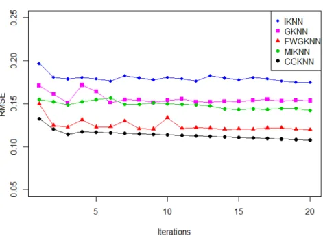
We provide a detailed analysis of how all the 6 algorithms performed in this simulation setting with n= 100, p= 5 and m = 4 classes in Table 2.3. Note that we used predictive mean matching as the imputation model for MICE. The plot for empirical convergence of the nearest neighbors algorithms are given in figure 2.3 when there is 20% missing data.
Table 2.3: RMSE Upon Convergence for the Toy MAR Dataset
Missing Rate MICE MissForest IKNN MI-KNN GKNN FWGKNN CGKNN
10% 0.1301 0.0902 0.1407 0.1071 0.1299 0.1229 0.0887
20% 0.2084 0.1177 0.1750 0.1423 0.1508 0.1196 0.1075
Figure 2.3: Convergence of RMSE for Nearest Neighbors Algorithms at 20% MAR
Table 2.4: Classification Accuracy (%) for MAR Dataset Missing Rate 10% 20%
No Imputation 75.13 72.50
MICE 79.09 77.32
MissForest 83.75 80.11
IKNN 85.48 83.91
MI-KNN 88.26 86.37
GKNN 86.38 84.12
FWGKNN 89.01 87.30
CGKNN 90.29 87.31
2.4 Applications to UCI Machine Learning Repository Datasets
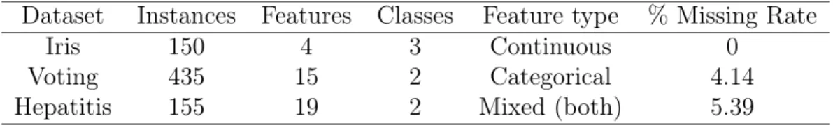
We evaluate the effectiveness of our imputation algorithm on 3 datasets obtained from UCI Machine Learning Repository (Newman et al. 2008), the Iris (Fisher’s Iris Dataset), Voting and Hepatitis datasets, having respectively, characteristics
Table 2.5: Characteristics of the UCI Datasets Used for Data Analysis Dataset Instances Features Classes Feature type % Missing Rate
Iris 150 4 3 Continuous 0
Voting 435 15 2 Categorical 4.14
Hepatitis 155 19 2 Mixed (both) 5.39
We represent the Mutual Information (MI) of each feature in these datasets in the graphs shown in Fig. 2.4 - 2.6, and use it as the weights for our CGKNN algorithm.
Figure 2.4: MI for the Sepal and Petal Lengths and Widths of Iris Dataset
Figure 2.6: MI for Hepatitis Dataset
We then introduce 3 different rates of artificial missingness at random (MAR) -5%, 10% and 20%. Then we run each of the imputation algorithms and calculate the RMSE of imputation after each algorithm converges. For MICE, we used predictive mean matching for continuous variables and polytomous logistic regression for categorical variables. Looking at Table 2.6 - Table 2.8 note that in almost all cases, our algorithm CGKNN performs better than the other algorithms, usually at higher percentages of missing values. MICE performs the worst in most cases, followed by MissForest, probably because they do not take into account any sort of feature relevance.
Table 2.6: Comparison of RMSE of Iris Dataset
Missing Rate MICE MissForest IKNN MI-KNN GKNN FWGKNN CGKNN
5% 0.0729 0.0619 0.0588 0.0503 0.0534 0.0506 0.0509
10% 0.1205 0.1302 0.1107 0.1025 0.1038 0.0995 0.0950
20% 0.1427 0.1420 0.1241 0.1146 0.1246 0.1106 0.1001
Table 2.7: Comparison of RMSE of Voting Dataset
Missing Rate MICE MissForest IKNN MI-KNN GKNN FWGKNN CGKNN
5% 0.0928 0.0919 0.0874 0.0791 0.0820 0.0770 0.0779
10% 0.1029 0.1002 0.0949 0.0870 0.0929 0.0868 0.0827
20% 0.1521 0.1601 0.1574 0.1446 0.1099 0.1088 0.1049
Table 2.8: Comparison of RMSE of Hepatitis Dataset
Missing Rate MICE MissForest IKNN MI-KNN GKNN FWGKNN CGKNN
5% 0.0913 0.0890 0.0785 0.0711 0.0792 0.0739 0.0714
10% 0.1029 0.1002 0.1107 0.0870 0.1038 0.0994 0.0921
20% 0.1967 0.1858 0.1592 0.0839 0.0980 0.0898 0.0823
algorithm also converges quite fast with respect to classification accuracy as shown in Fig. 2.7.
2.5 Discussion
Missing data is a classical drawback for most classification algorithms. However, most of the missing data imputation techniques have been developed without taking into account the class information, which is always present for a supervised machine learning problem. k-Nearest Neighbors is a good technique for imputation of missing data and has shown to perform well against many other imputation procedures. We have proposed a method which not only takes into account the class information, but also uses a better metric to calculate the nearest neighbors in KNN imputation. Our Class-weighted Greyk-Nearest Neighbor (CGKNN) approach has same time
complexity as the previous algorithms and even better than some KNN imputation algorithms like Grey-Based k-Nearest Neighbor (GBNN) and Iterativek-Nearest Neighbor (IKNN) imputation. We have shown that it outperforms all the other algorithms in simulated settings, as well as high rates of missingness in actual (non-simulated) datasets as far as imputation is concerned. We also show that it improves the accuracy of classification better than other imputation procedures. We do not make any assumptions regarding the variables of the feature matrix and thus, for any classification problem, our method can be used to impute missing data in the feature matrix.
theoretical problem to consider.
Another potentially interesting future research topic would be to extend this idea to regression problem where the outcome Y is continuous instead of categorical. The imputation of the data matrix X could be done with the help of information fromY since they are assumed to be related in a regression setting. We could also look into better methods of measuring the relationship between the features and class variable than mutual information (MI) and then use them as weights for the Grey distance. Another potential future research paper is to develop an algorithm which imputes and classifies simultaneously, thus yielding a better classification in a single step instead of imputation and classification at two different stages. This idea has already been worked on in Learning Vector Quantization (LVQ) (Villmann et al. 2006) but can be vastly improved.
CHAPTER 3: RANDOM FOREST IMPUTATION OF MISSING COVARIATES FOR LONGITUDINAL DATA MODELS
3.1 Introduction
Longitudinal studies are prone to huge losses or missingness in terms of the number of participants due to follow up. Particularly in older populations, the reason for this loss to follow up is death. The other reasons may be serious like loss of
mobility, shifting to a different part of the country, loss of memory or may be trivial like non-compliance. For all reasons other than death, the participants may be called up to partially recover the data, without a proper physical visit. An example is the Atherosclerosis Risk in Communities (ARIC) Study Cohort where there are 15,792 participants who took part in the 1st visit back in 1987-1989 across 4 states in the USA (ARIC investigators 1989) and only 6,538 people returned for the 5th visit in 2011-2013, which represents just 41.7 % of the original number of participants. For these 6,538 participants, diabetes was an outcome which was universally measured and a lot of other covariates were taken like blood pressure, glucose levels, etc. But these covariates had some missingness due to non-response (during the visit), storage problems or fault of the data collector. For the remaining 9,254 participants, those who were alive were called up to partially collect data on covariates for which physical visit was not needed. Diabetes status was ascertained for some of these 9,254 patients lost to follow-up, along with a few covariate values. However, most covariate values could not be recorded.
for some of the participants due to lack of a physical visit or other data recording problems. As shown in many studies (Enders 2010), ignoring observations with missing values and going ahead with the inference problem to be addressed leads to a loss of power and information. Some imputation problems are only for continuous data (Aittokallio 2009) whereas many parametric imputation techniques have a high computational complexity (Liao et al. 2014). Most of the parametric techniques have a bias associated with it if the model is misspecified. To ease the restrictions, fully conditional specification of the covariates had been used, but it is not easy to specify for complicated interactions (Bartlett et al. 2015).
Due to the complexities of dealing with imputation parametrically,
dropout those who died before being examined at the next ARIC visit.
The first research done in machine learning-based imputation of longitudinal data was using Partial Logistic Artificial Neural Network (PLANN) regularised within the evidence-based framework with Automatic Relevance Determination (ARD), together known as PLANN-ARD (Fernandes et al. 2008). For the simplicity and robustness of non-parametric methods, machine learning methods have been often preferred in missing data imputation. A promising approach can be random forests, developed first by Tin Kam Ho and then worked on by Breiman (Breiman 2001) and patented on by Adele Cutler (3185828).
Random forests have a huge advantage over traditional machine learning algorithms because it is comparatively faster to train, addresses complicated non-linear interactions, handles mixed data type and can easily scale to high
dimensions without over-fitting. Random forest as an imputation technique has been studied before. The performance of the imputation technique is given by the
Out-of-Bag (OOB) error of the RF models used in imputation. The first stride in random forest imputation was using the proximity algorithm by the R-package randomForest developed from Breiman’s original idea (Liaw et al. 2002). The next approach in this area was using “on-the-fly imputation” algorithm which involves growing a survival tree simultaneously while imputing the missing values in the dataset (Ishwaran and Lu 2008). The third approach involves unsupervised learning in the imputation problem, where each covariate is treated as a dependent variable which is the outcome of a random forest grown from the other covariates. This approach is called missForest (Stekhoven and Bühlmann 2011) and is quite popular since it has been shown to outperform MICE and IKNN (Iterative k-Nearest
Neighbors) algorithms.
using random splits while growing the tree to increase the computational speed of the methods (Tang and Ishwaran 2017). We apply various random forest imputation methods to simulated longitudinal datasets with datapoints missing both completely at random (MCAR) and at random (MAR). We compare the performance with traditional non-parametric imputation techniques like MICE (Buuren and Oudshoorn 1999) and iterative kNN (IKNN) (Troyanskaya et al. 2001).
The remainder of this chapter is organized as follows. In Section 2, we formally state the problem of missingness in longitudinal data and then propose the various imputation techniques using random forests. We shall show the variant of random forest imputation which we propose for longitudinal data. In Section 3, we test our proposed imputation methods, including their randomized versions, against MICE and Iterative kNN (IKNN) imputation in various simulation settings with data missing completely at random and at random. We check how our method performed against all the other methods. We conclude with a discussion of application to the ARIC dataset and scope for future work in Section 4.
3.2 Methodology
3.2.1 Formulation of the Problem
As stated before, we deal with longitudinal datasets where the response is observed or recorded for each timepoint either by a physical visit or phone call. Due to various reasons, the covariate values may be missing partially or wholly for a few participants at certain timepoints. Let X ={Xijk}n
i=1 be the n×t×p data matrix whereXijk represents thek-th covariate of the i-th subject/individual at time pointj. We assume there are n individuals, p covariates and t time points. Similarly,
response at time point j. Y can be a continuous or categorical variable observed across t timepoints. There are n subjects for t time points. We consider the longitudinal data{(Xijk, Yij)}n
i=1 with n subjects. We assume the following model to be satisfied by the data
E(Yij|Xij) =f(Xij), i={1,2, ..., n}, j ={1,2, ..., t}, (3.1)
wheref(.)is a continuous or categorical real-valued function, Xij ={Xijk}pk=1 has
missing entries and Y is completely observed. Now, there may be demographic covariates inX which do not change with time and are recorded for each of the n subjects in the initial visit. We still make t copies of these demographic variables so that the data matrix X has a dimension of n×t×p and is easier for notation - but it will be treated differently during imputation as we will soon explain.
We denote the missing entries in the data matrixX by the indicator matrix D={Dijk}ni=1 with same dimensionality as X and
Dijk =
0, Xijk is missing 1, otherwise.
(3.2)
We assume the data matrix contains mixed-type data. Without loss of generality, we can assume for each (i, j) pair, the subject Xij ={Xijk}pk=1 contains p0 categorical features forj ∈ {1,2, ..., p0} and p1 continuous features for j ∈ {p0+ 1, ..., p0+p1} such thatp0+p1 =p. Let the j-th categorical feature contain kj different values and the j-th continuous variable representing the (p0+j)-th feature of Xi, indexed by j ∈ {1, ..., p1} take values from a continuous setCj ⊂R. For each of the categorical
We assume that the data is missing at random (MAR), that is, the distribution of D does not depend on the missing values inX but rather the observed values,
P(D|X) = P(D|Xobs), for all Xmis (3.3)
We propose tree-based approaches to impute the n×t×p data matrix X, since it will have complicated interactions between the pdimensional covariates
{Xij}, i= 1,2, ..., n, j = 1,2, ..., t.. Decision trees divide the feature matrix intuitively into classes and assigns a predicted value to each partition (Friedman et al. 2001). Classification and Regression Trees (CART) have been built in 1984 (Breiman et al. 1984) as a reproducible method to use decision trees to model the outcome variable. We then move on to random forest (RF), first introduced by Tin Kam Ho (Ho 1995), and later developed by Leo Breiman (Breiman 2001) and Adele Cutler who registered “Random Forests” as a trademark (3185828), which aggregates several trees that make decisions after some random selection at each internal tree node.
3.2.2 Classification and Regression Trees (CART)
In this section, we generally state how Classification and Regression Trees
those with {X..k > c} fall into the other area made by the split. A splitting point is called an internal node. The terminal nodes are the final end points.
We can define the regions in the partitioned data matrixX as Rm, m= 1, ..., M, whereM is the number of terminal nodes. Let the average outcome of the terminal nodem be written as
b
cm = n X i=1 t X j=1
YijI{Xij. ∈Rm}
Pn
a=1
Pt
b=1I{Xab.∈Rm} ,
then we may estimate f(Xij) =E[Yij|Xij]with
b
f(Xij) = M
X
m=1
b
cmI{Xij. ∈Rm}.
So the predicted value of a new data point is equal to the average of observed
outcomes across all training set data points, over all different timepoints, in the same terminal node as the new data point.
In the greedy approach to build a tree, all thep variables and their possible cut points are considered at each node, and we move forward with the cut point which gives a maximum gain in terms of a suitable criteria. To choose the variable and cut point for each node, minimization of the sum of squares is performed:
min k,c min a X
i,j:Xij.∈Rl(k,c)
(Yij −a)2+ min b
X
i,j:Xij.∈Rg(k,c)
(Yij −b)2
,
given in section 3.2.4. The stopping criteria for tree growth is a minimum (terminal) node size. In other words, a terminal node must have at least the minimum node size. When all terminal nodes can no longer be split, growing the tree is completed, and we call this the maximal treeT0.
To decrease over-fitting, cost-complexity pruning is then used to cut back the maximal tree. DefineT to be a subtree of T0, and |T| to be the total number of nodes
in the tree T. A sequence of subtrees is constructed by sequentially collapsing non-terminal nodes that lead to the smallest value of
1 M M X m=1 X
i,j:Xij.∈Rm
(Yij −bcm)
2.
The tree within this sequence that minimizes the cost complexity criterion,
Cα(T) = M
X
m=1
X
i,j:Xij.∈Rm
(Yij −bcm)
2+αM,
is then selected as the final tree. α may be chosen by minimizing the cross-validated sum of squares.
The above concept of regression may also be extended to classification (since the name is Classification and Regression Trees) in longitudinal studies where the
splitting criteria are based on node impurity measures such as misclassification error or Gini index. The predicted class of a data point in a classification problem withK distinct classes is
arg max k∈1:K
{pbmk},
wherepbmk is the proportion of observations in terminal nodem with the classk. In