Lecture 14
Least squares estimation
Plan of the lecture:
1. Estimator
1.1 Point estimators 1.2 Consistency
1.3 Asymptotic normality 1.4 Efficiency
1.5 Robustness 1.6 Other properties 2. Least squares estimation
1 Estimator
In statistics, an estimator is a statistic (a function of the observable sample data) that is used to estimate an unknown population parameter (which is called the estimand); an estimate is the result from the actual application of the function to a particular sample of data.
It is possible to construct many estimators for a given parameter: the construction and comparison of estimators forms estimation theory. In the context of decision theory, an estimator is a type of decision rule, and the performance of an estimator may be evaluated through the use of loss functions.
To estimate a parameter of interest (e.g., a population mean, a binomial proportion, a difference between two population means, or a ratio of two population standard deviations), the usual procedure is as follows:
1. Select a random sample from the population of interest. 2. Calculate the point estimate of the parameter.
3. Calculate a measure of its variability, often a confidence interval. 4. Associate with this estimate a measure of variability.
There are many types of estimators, including point estimators, interval estimators,
density estimators, as well as function estimators.
1.1 Point estimators
Suppose we have a fixed parameter that we wish to estimate. Then an estimator is a function that maps a sample design to a set of sample estimates. An estimator of is usually denoted by the symbol . A sample design can be thought of as an ordered pair where is
a set of samples (or outcomes), and is the probability density function. The probability density
function maps the set to the closed interval , and has the property that the sum (or integral) of the values of , over all in , is equal to . For any given subset of , the sum or integral of over all in is .
For all the properties below, the value , the estimation formula, the set of samples, and
the set probabilities of the collection of samples, can be considered fixed. Yet since some of the definitions vary by sample (yet for the same set of samples and probabilities), we must use in the notation. Hence, the estimate for a given sample is denoted as .
1. For a given sample , the error of the estimator is defined as , where is
the estimate for sample , and is the parameter being estimated. Note that the error depends not only on the estimator (the estimation formula or procedure), but on the sample.
2. The mean squared error of is defined as the expected value (probability-weighted
average, over all samples) of the squared errors; that is, . It is
used to indicate how far, on average, the collection of estimates are from the single parameter being estimated. Consider the following analogy. Suppose the parameter is the bull's-eye of a target, the estimator is the process of shooting arrows at the target, and the individual arrows are estimates (samples). Then high means the average distance of the arrows from the bull's-eye is high, and low means the average distance from the
bull's-eye is low. The arrows may or may not be clustered. For example, even if all arrows hit the same point, yet grossly miss the target, the is still relatively large. Note, however, that if the is relatively low, then the arrows are likely more highly
clustered (than highly dispersed).
3. For a given sample , the sampling deviation of the estimator is defined as , where is the estimate for sample , and is the expected value of the
estimator. Note that the sampling deviation depends not only on the estimator, but on the sample.
4. The variance of is simply the expected value of the squared sampling deviations; that
is, . It is used to indicate how far, on average, the collection
of estimates are from the expected value of the estimates. Note the difference between and variance. If the parameter is the bull's-eye of a target, and the arrows are
estimates, then a relatively high variance means the arrows are dispersed, and a relatively low variance means the arrows are clustered. Some things to note: even if the variance is low, the cluster of arrows may still be far off-target, and even if the variance is high, the diffuse collection of arrows may still be unbiased. Finally, note that even if all arrows grossly miss the target, if they nevertheless all hit the same point, the variance is zero.
5. The bias of is defined as . It is the distance between the average of the collection of estimates, and the single parameter being estimated. It also is the
expected value of the error, since . If the parameter is the
bias means the average position of the arrows is on target. They may be dispersed, or may be clustered. The relationship between bias and variance is analogous to the
relationship between accuracy and precision.
6. is an unbiased estimator of if and only if . Note that bias is a property of
the estimator, not of the estimate. Often, people refer to a "biased estimate" or an "unbiased estimate," but they really are talking about an "estimate from a biased estimator," or an "estimate from an unbiased estimator." Also, people often confuse the "error" of a single estimate with the "bias" of an estimator. Just because the error for one estimate is large, does not mean the estimator is biased. In fact, even if all estimates have astronomical absolute values for their errors, if the expected value of the error is zero, the estimator is unbiased. Also, just because an estimator is biased, does not preclude the error of an estimate from being zero (we may have gotten lucky). The ideal situation, of course, is to have an unbiased estimator with low variance, and also try to limit the number of samples where the error is extreme (that is, have few outliers). Yet unbiasedness is not essential. Often, if we permit just a little bias, then we can find an estimator with lower and/or fewer outlier sample estimates.
7. The , variance, and bias, are related: , i.e.
. In particular, for an unbiased estimator, the variance equals the .
8. The standard deviation of an estimator of (the square root of the variance), or an estimate of the standard deviation of an estimator of , is called the standard error of .
1.2 Consistency
A consistent sequence of estimators is a sequence of estimators that converge in probability to the quantity being estimated as the index (usually the sample size) grows without bound. In other words, increasing the sample size increases the probability of the estimator being close to the population parameter.
Mathematically, a sequence of estimators is a consistent estimator for parameter if and only if, for all , no matter how small, we have
The consistency defined above may be called weak consistency. The sequence is
strongly consistent, if it converges almost surely to the true value.
An estimator that converges to a multiple of a parameter can be made into a consistent estimator by multiplying the estimator by a scale factor, namely the true value divided by the asymptotic value of the estimator. This occurs frequently in estimation of scale parameters by measures of statistical dispersion.
1.3 Asymptotic normality
An asymptotically normal estimator is a consistent estimator whose distribution around the true parameter approaches a normal distribution with standard deviation shrinking in
proportion to as the sample size grows. Using to denote convergence in distribution, is asymptotically normal if
,
for some , which is called the asymptotic variance of the estimator.
The central limit theorem implies asymptotic normality of the sample mean as an estimator of the true mean. More generally, maximum likelihood estimators are asymptotically normal under fairly weak regularity conditions.
1.4 Efficiency
Two naturally desirable properties of estimators are for them to be unbiased and have minimal mean squared error ( ). These cannot in general both be satisfied simultaneously: a biased estimator may have lower mean squared error ( ) than any unbiased estimator: despite
having bias, the estimator variance may be sufficiently smaller than that of any unbiased estimator, and it may be preferable to use, despite the bias.
Among unbiased estimators, there often exists one with the lowest variance, called the minimum variance unbiased estimator ( ). In some cases an unbiased efficient estimator
exists, which, in addition to having the lowest variance among unbiased estimators, satisfies the Cramér-Rao bound, which is an absolute lower bound on variance for statistics of a variable.
Concerning such "best unbiased estimators", see also Cramér-Rao bound, Gauss-Markov
1.5 Robustness
Strictly speaking, a robust statistic is resistant to errors in the results, produced by deviations from assumptions (e.g. of normality). This means that if the assumptions are only approximately met, the robust estimator will still have a reasonable efficiency, and reasonably small bias, as well as being asymptotically unbiased, meaning having a bias tending towards as
the sample size tends towards infinity.
1.6 Other properties
Sometimes, estimators should satisfy further restrictions (restricted estimators) – e.g., one might require an estimated probability to be between zero and one, or an estimated variance to be nonnegative. Sometimes this conflicts with the requirement of unbiasedness.
2 Least squares estimation
In many practical contexts, we want to form an estimate of the value of a random variable given the value of a related random variable , which may be viewed as some form of “measurement” of . For example, may be the range of an aircraft and may be a
noise-corrupted measurement of that range. In this section we discuss a popular formulation of the estimation problem, which is based on finding the estimate that minimizes the expected value of the squared error (hence the name “least squares”).
If the value of is not available, we may consider finding an estimate (or prediction) of . The estimation error is random (because is random), but the mean squared error is a number that depends on and can be minimized over . With respect to this criterion, it turns out that the best possible estimate is , as we proceed to verify.
Let . For any estimate , we have
)2= ( )2+2 +( )2= ( )2+( )2,
where we used the fact . The first term in the right-hand side is the variance of
Figure 1: The mean squared error , as a function of the estimate , is a quadratic in
and is minimized when . The minimum value of the mean squared error is .
Suppose now that we observe the experimental value of some related random variable , before forming an estimate of . How can we exploit this additional information? Once we are told that takes a particular value , the situation is identical to the one considered earlier, except that we are now in a new “universe,” where everything is conditioned on . We can therefore adapt our earlier conclusion and assert that minimizes the conditional
mean squared error . Note that the resulting estimate depends on the experimental value of (as it should). Thus, we call the least-squares estimate of
given the experimental value .
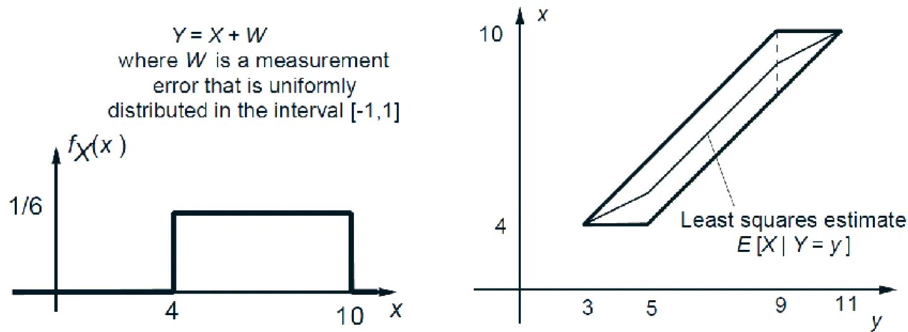
Example 1. Let be uniformly distributed in the interval and suppose that we observe with some random error , that is, we observe the experimental value of the random variable .
We assume that is uniformly distributed in the interval , and independent of . What is the least squares estimate of given the experimental value of ?
We have for , and , elsewhere. Conditioned on being equal to some , is the same as , and is uniform over the interval .
Thus, the joint PDF is given by
,
Given an experimental value of , the conditional PDF of is uniform on the corresponding vertical section of the slanted rectangle. The optimal estimate is the
midpoint of that section. In the special case of the present example, it happens to be a piecewise linear function of .
Figure 2: The PDFs in Example 1. The least squares estimate of given the experimental value of the random variable depends on and is represented by the piecewise linear
function shown in the figure on the right.
As Example 1 illustrates, the estimate depends on the observed value and should be viewed as a function of ; see Fig. 3. To amplify this point, we refer to any function of
the available information as an estimator. Given an experimental outcome of , an estimator (which is a function) produces an estimate (which is a number). However, if is left
unspecified, then the estimator results in a random variable . The expected value of the squared estimation error associated with an estimator is
.
Out of all estimators, it turns out that the mean squared estimation error is minimized when . To see this, note that if is any number, we have
.
.
This inequality is true for every possible experimental value of . Thus,
,
which is now an inequality between random variables (functions of ). We take expectations of
both sides, and use the law of iterated expectations, to conclude that
for all functions .
Figure 3: The least squares estimator.
Key Facts about Least Mean Squares Estimation
is minimized when :
, for all .
is minimized when :
, for all .
Out of all estimators of based on , the mean squared estimation error
is minimized when :
, for all functions .
Let us introduce the notation
, ,
for the (optimal) estimator and the associated estimation error, respectively. Note that both and are random variables, and by the law of iterated expectations,
.
The equation remains valid even if we condition on , because
.
We have used here the fact that is completely determined by and therefore . For similar reasons,
.
Taking expectations and using the law of iterated expectations, we obtain
.
Note that , which yields . We square both sides of
the latter equality and take expectations to obtain
.
(The last equality holds because and .) In summary, we have
established the following important formula, which is just another version of the law of conditional variances.
Example 2. Let us say that the observed random variable is uninformative if the mean squared estimation error is the same as the unconditional variance of .
When is this the case? Using the formula
,
we see that is uninformative if and only if . The variance of a random variable is zero if and only if that random variable is a constant, equal to its mean. We conclude that is uninformative if and only if , for every realization of .
If and are independent, we have and is indeed uninformative, which is quite intuitive. The converse, however, is not true. That is, it is possible for to be always equal to the constant , without and being independent.
Estimation Based on Several Measurements
So far, we have discussed the case where we estimate one random variable on the basis
of another random variable . In practice, one often has access to the experimental values of
several random variables , that can be used to estimate . Generalizing our earlier discussion, and using essentially the same argument, the mean squared estimation error is minimized if we use as our estimator. That is,
, for all functions .
This provides a complete solution to the general problem of least squares estimation, but is sometimes difficult to implement, because:
(a) In order to compute the conditional expectation , we need a complete probabilistic model, that is, the joint PDF of random variables.
(b) Even if this joint PDF is available, can be a very complicated function of .
.
Given a particular choice of , …, , , the corresponding mean squared error is
,
and it is meaningful to choose the coefficients , …, , , in a way that minimizes the above
expression. This problem is relatively easy to solve and only requires knowledge of the means, variances, and covariances of the different random variables. We develop the solution for the case where .
Linear Least Mean Squares Estimation Based on a Single Measurement
We are interested in finding and that minimize the mean squared estimation error , associated with a linear estimator of . Suppose that has already
been chosen. How should we choose ? This is the same as having to choose a constant to
estimate the random variable and, by our earlier results, the best choice is to let .
It now remains to minimize, with respect to , the expression
,
which is the same as
[ ] [ ]= 2+ 2 2 2 cov( , ),
where is the covariance of and :
.
This is a quadratic function of , which is minimized at the point where its derivative is
,
where
is the correlation coefficient. With this choice of , the mean squared estimation error is given by
.
Linear Least Mean Squares Estimation Formulas
The least mean squares linear estimator of based on is
.
The resulting mean squared estimation error is equal to