A Rough Set View on Bayes’ Theorem
Zdzisław Pawlak*University of Information Technology and Management, ul. Newelska 6, 01 447 Warsaw, Poland
Rough set theory offers new perspective on Bayes’ theorem. The look on Bayes’ theorem offered by rough set theory reveals that any data set (decision table) satisfies the total probability theorem and Bayes’ theorem. These properties can be used directly to draw conclusions from objective data without referring to subjective prior knowledge and its revision if new evidence is available. Thus, the rough set view on Bayes’ theorem is rather objective in contrast to subjective “classical” interpretation of the theorem. © 2003 Wiley Periodicals, Inc.
MOTTO: “It is a capital mistake to theorise before one has data” Sherlock Holmes (A Scandal in Bohemia)
1. INTRODUCTION
This article is a continuation of some ideas presented in Ref. 1, which were inspired by the research of Łukasiewicz on the relationship between logic and probability.2 He first pointed out connections between implication and Bayes’
theorem. His observation is the starting point of the approach presented in this study. Before we start our considerations, let us briefly recall some facts and opinions about Bayes’ theorem.
In his article3Bayes considered the following problem: “Given the number of
times in which an unknown event has happened and failed: required the chance that the probability of its happening in a single trial lies somewhere between any two degrees of probability that can be named.”
In fact “. . . it was Laplace (1774 –1886)—apparently unaware of Bayes’ work—who stated the theorem in its general (discrete) form”.4
Bayes’ theorem has the following form
P共H兩D兲⫽P共D兩H兲⫻P共H兲/P共D兲 *e-mail: [email protected].
INTERNATIONAL JOURNAL OF INTELLIGENT SYSTEMS, VOL. 18, 487– 498 (2003) © 2003 Wiley Periodicals, Inc. Published online in Wiley InterScience
where P(H) is called the prior probability of a hypothesis H and expresses our knowledge aboutH before having dataD; P(H兩D)— called the posterior proba-bility ofH givenD—tells us what is known about H after obtaining data.
Currently, Bayes’ theorem is the basis of statistical interference. “The result of the Bayesian data analysis process is the posterior distribution that represents a revision of the prior distribution on the light of the evidence provided by the data”.5
Bayes’-based inference methodology raised much controversy and criticism, e.g., “Opinion as to the values of Bayes’ theorem as a basis for statistical inference has swung between acceptance and rejection since its publication in 1763.”6
“The technical results at the heart of the essay is what we now know asBayes’ theorem.However, from a purely formal perspective there is no obvious reason why this essentially trivial probability result should continue to excite interest”.4
Rough set theory offers new insight into Bayes’ theorem. The look on Bayes’ theorem presented here is completely different from that used in the Bayesian data analysis philosophy. It does not refer either to prior or posterior probabilities, inherently associated with Bayesian reasoning, but it reveals some probabilistic structure of the data being analyzed. It states that any data set (decision table) satisfies total probability theorem and Bayes’ theorem. This property can be used directly to draw conclusions from data without referring to prior knowledge and its revision if new evidence is available. Thus, in the presented approach the only source of knowledge is the data and there is no need to assume that there is any prior knowledge besides the data.
Moreover, the proposed approach to Bayes’ theorem shows a close relation-ship between logic of implications and probability, which was first observed by Łukasiewicz2 and also independently studied by Adams7 and others. Bayes’
theorem in this context can be used to “invert” implications, i.e., to give reasons for decisions. This is a very important feature of utmost importance to data mining and decision analysis, because it extends the class of problem, which can be considered in these domains.
Besides, we propose a new form of Bayes’ theorem in which the basic role is played by strength of decision rules (implications) derived from the data. The strength of decision rules is computed from the data or it also can be a subjective assessment. This formulation gives a new look on Bayesian method of inference and also simplifies essentially computations.8
It is also interesting to note a relationship between Bayes’ theorem and flow graphs.
Let us also observe that the rough set view on Bayes’ theorem is rather objective in contrast to subjective “classical” interpretation.
2. INFORMATION SYSTEMS AND APPROXIMATION OF SETS
In this section we define basic concepts of rough set theory: information system and approximation of sets. Rudiments of rough set theory can be found in Ref. 1.
An information system is a data table in which its columns are labeled by attributes, rows are labeled by objects of interest, and entries of the table are attribute values.
Formally, by an information system we will understand a pair S ⫽ (U, A), where U and A are finite, nonempty sets called the universe and the set of attributes, respectively. With every attribute a 僆 A we associate a set Va of its values, called the domain ofa. Any subsetBofAdetermines a binary relationI(B) onU, which will be called an indiscernibility relation and is defined as follows: (x, y) 僆 I(B) if and only ifa(x) ⫽ a(y) for everya 僆 A, where a(x) denotes the value of attributeafor elementx. Obviously,I(B) is an equivalence relation. The family of all equivalence classes ofI(B), i.e., a partition determined byB, will be denoted byU/I(B) or simply byU/B; an equivalence class ofI(B), i.e., block of the partitionU/B, containingx will be denoted byB(x).
If (x, y) belongs to I(B) we will say that x and y are B-indiscernible (indiscernible with respect to B). Equivalence classes of the relation I(B) (or blocks of the partitionU/B) are referred to as B-elementary sets or B-granules.
If we distinguish in an information system two disjoint classes of attributes, called condition and decision attributes, respectively, then the system will be called a decision table and will be denoted byS⫽(U,C,D), whereCandDare disjoint sets of condition and decision attributes, respectively.
Thus, the decision table determines decisions that must be taken when some conditions are satisfied. In other words, each row of the of the decision table specifies a decision rule that determines decisions in terms of conditions.
Observe that elements of the universe, in the case of decision tables, are simply labels of decision rules.
Suppose we are given an information systemS ⫽(U,A),X債 U, andB 債 A. Our task is to describe the setXin terms of attribute values fromB. To this end, we define two operations assigning to everyX 債 U two sets B
*(X) and B*(X) called the B-lower and the B-upper approximation of X, respectively, and are defined as follows:
B
*共X兲⫽
艛
x僆U 兵B共x兲 : B共x兲債X其 B*共X兲⫽艛
x僆U
兵B共x兲 : B共x兲艚X⫽A其
Hence, theB-lower approximation of a set is the union of allB-granules that are included in the set, whereas theB-upper approximation of a set is the union of all B-granules that have a nonempty intersection with the set. The set
BNB共X兲⫽B*共X兲⫺B*共X兲 will be referred to as theB-boundary region ofX.
If the boundary region ofXis the empty set, i.e.,BNB(X)⫽A, thenXis crisp (exact) with respect toB; in the opposite case, i.e., ifBNB(X) ⫽ A, Xis referred to as rough (inexact) with respect toB.
3. ROUGH MEMBERSHIP
Rough sets also can be defined using rough membership function instead of approximations,9which is defined as follows:
X
B: U 3 关0, 1兴 and
X
B共x兲⫽兩B共x兲艚X兩 兩B共x兲兩
where X 債 U andB 債 A and兩X兩 denotes the cardinality ofX.
The function measures the degree thatxbelongs toXin view of information aboutx expressed by the set of attributesB.
The rough membership function has the following properties:
(1) X B
(x) ⫽ 1 iffx僆 B *(X) (2) X
B
(x) ⫽ 0 iffx 僆U ⫺ B*(X) (3) 0 ⬍ X
B
(x) ⬍ 1 iffx 僆 BNB(X)
(4) U⫺X B
(x) ⫽ 1⫺ X B
(x) for anyx 僆 U (5) X艛Y
B
(x) 肁 max(X B
(x), Y B
(x)) for any x僆 U (6) X艚Y
B
(x) 聿 min(X B
(x),Y B
(x)) for anyx 僆 U
Compare these properties with those of fuzzy membership. Obviously, rough membership is a generalization of fuzzy membership.
The rough membership function can be used to define approximations and the boundary region of a set, as shown below:
B*共X兲⫽兵x僆U :X B共
x兲⫽1其 B*共X兲⫽兵x僆U: X
B共 x兲⬎0其 BNB共X兲⫽兵x僆U: 0⬍X
B共 x兲⬍1其
4. INFORMATION SYSTEMS AND DECISION RULES
Every decision table describes decisions determined when some conditions are satisfied. In other words, each row of the decision table specifies a decision rule that determines decisions in terms of conditions.
Let us describe decision rules more exactly. LetS⫽(U,C,D) be a decision table. Everyx僆U determines a sequencec1(x), . . . ,cn(x),d1(x), . . . ,dm(x), where {c1, . . . , cn} ⫽ C and {d1, . . . , dm} ⫽ D. The sequence will be called a decision rule induced by x (in S) and denoted by c1(x), . . . , cn(x) 3 d1(x), . . . , dm(x) or, in short,C 3x D.
The number suppx(C, D) ⫽ 兩C(x) 艚 D(x)兩 will be called a support of the decision rule C3x D and the number
x共C, D兲⫽
suppx共C,D兲 兩U兩 490
will be referred to as the strength of the decision ruleC3xD. With every decision ruleC3xD, we associate the certainty factor of the decision rule, denoted cerx(C, D) and defined as follows:
cerx共C,D兲⫽
兩C共x兲艚D共x兲兩 兩C共x兲兩 ⫽
suppx共C,D兲 兩C共x兲兩 ⫽
x共C,D兲 共C共x兲兲 where (C(x)) ⫽ [兩C(x)兩/兩U兩].
The certainty factor may be interpreted as a conditional probability that y belongs to D(x) given y belongs toC(x), symbolically x(D兩C).
If cerx(C, D) ⫽ 1, thenC 3x D will be called a certain decision rule inS; if 0⬍cerx(C,D)⬍1, the decision rule will be referred to as an uncertain decision rule inS. Furthermore, we will also use a coverage factor10 of the decision rule,
denoted covx(C, D), defined as
covx共C,D兲⫽
兩C共x兲艚D共x兲兩 兩D共x兲兩 ⫽
suppx共C,D兲 兩D共x兲兩
⫽x共C,D兲
共D共x兲兲
where (D(x)) ⫽ [兩D(x)兩/兩U兩]. Similarly,
covx共C,D兲⫽x共C兩D兲
IfC3xD is a decision rule, thenD3xCwill be called an inverse decision rule. The inverse decision rules can be used to give explanations (reasons) for decisions.
Let us observe that
cerx共C,D兲⫽DC共x兲共x兲 and covx共C,D兲⫽CD共x兲共x兲
Moreover, it is worthwhile to mention that the certainty factor of a decision rule C 3x D is, in fact, the coverage factor of the inverse decision rule D 3x C.
That means that the certainty factor expresses the degree of membership ofx to the decision class D(x), given C, whereas the coverage factor expresses the degree of membership ofx to condition classC(x), givenD.
Decision rules often are represented in a form of “if, . . . , then, . . . ,” impli-cations. Thus, any decision table can be transformed in a set of “if, . . . , then, . . . ,” rules, called a decision algorithm.
Generation of minimal decision algorithms from decision tables is a complex task and we will not discuss this issue here. The interested reader is advised to consult the references, e.g., Ref. 11.
5. PROBABILISTIC PROPERTIES OF DECISION TABLES
Decision tables have important probabilistic properties, which are discussed next.
LetC3x Dbe a decision rule inSand let⌫ ⫽C(x) and⌬ ⫽ D(x). Then, the following properties are valid:
冘
y僆⌫
cery共C,D兲⫽1 (1)
冘
y僆⌬
covy共C,D兲⫽1 (2)
共D共x兲兲⫽
冘
y僆⌫
cery共C,D兲䡠共C共y兲兲
⫽
冘
y僆⌫
y共C,D兲 (3)
共C共x兲兲⫽
冘
y僆⌬
covy共C,D兲䡠共D共y兲兲
⫽
冘
y僆⌬
y共C, D兲 (4)
cerx共C,D兲⫽
covx共C,D兲䡠共D共x兲兲 ¥y僆⌬covy共C,D兲䡠共D共y兲兲
⫽x共C, D兲
共C共x兲兲 (5)
covx共C,D兲⫽
cerx共C,D兲䡠共C共x兲兲 ¥y僆⌫cery共C,D兲䡠共C共y兲兲
⫽x共C, D兲
共D共x兲兲 (6)
That is, any decision table, satisfies Equations 1– 6. Observe that Equations 3 and 4 refer to the well-known total probability theorem, whereas Equations 5 and 6 refer to Bayes’ theorem.
Thus, to compute the certainty and coverage factors of decision rules accord-ing to Equations 5 and 6, it is enough to know the strength (support) of all decision rules only. The strength of decision rules can be computed from data or can be a subjective assessment.
6. DECISION TABLES AND FLOW GRAPHS
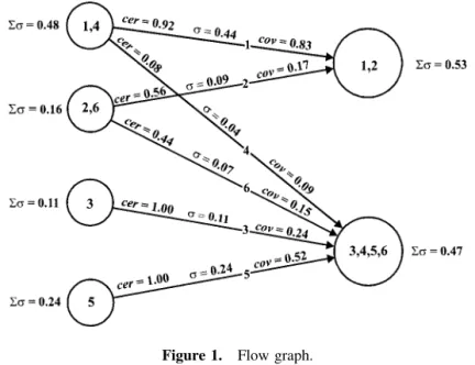
With every decision table, we associate a flow graph, i.e., a directed, con-nected, acyclic graph defined as follows: to every decision ruleC3xD, we assign a directed branch x connecting the input node C(x) and the output node D(x). With every branchxof the flow graph, we associate the number␥(x)⫽x(C,D), called throughflow of x. The throughflow of the graph is governed by Equations 1– 6.
Equations 1 and 2 are obvious. Equation 3 states that the outflow of the output node amounts to the sum of its inflows, whereas Equation 4 says that the sum of outflows of the input node is equal to its inflow. Finally, Equations 5 and 6 reveal how throughflow in the flow graph is distributed between its inputs and outputs.
Observe that Equations 1– 6 can be regarded as flow conservation equations similar to those introduced by Ford and Fulkerson12in flow networks. However, flow graphs introduced in this study differ essentially from flow networks and refer to other aspects of flow than those considered in Ref. 12.
In addition, let us mention that the concept of the flow graph can be formulated in more general terms, independently from decision tables and it can find quite new applications.
7. ILLUSTRATIVE EXAMPLES
Now we will illustrate the ideas considered in the previous sections by simple tutorial examples. These examples intend to show clearly the difference between “classical” Bayesian approach and that proposed by the rough set philosophy.
Example 1. This example will show clearly the different role of Bayes’ theorem in classical statistical inference and that in rough set– based data analysis.
Let us consider the data table shown in Table I. In Table I the number of patients belonging to the corresponding classes is given. Thus, we start from the original data (not probabilities) representing outcome of the test.
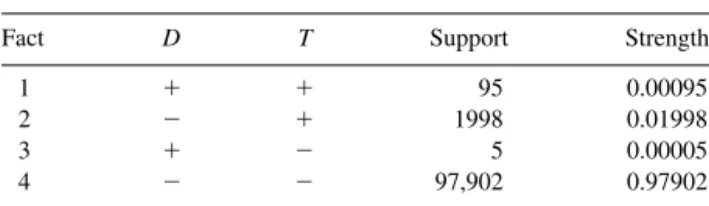
Now, from Table I we create a decision table and compute strength of decision rules. The results are shown in Table II. In Table II,D is the condition attribute, whereas T is the decision attribute. The decision table is meant to represent a “cause-effect” relation between the disease and the result of the test. That is, we expect that the disease causes a positive test result and lack of the disease results in negative test result.
The decision algorithm is given below: Table I. Data table.
T⫹ T⫺
D 95 5
D 1998 97,902
Table II. Decision table.
Fact D T Support Strength
1 ⫹ ⫹ 95 0.00095
2 ⫺ ⫹ 1998 0.01998
3 ⫹ ⫺ 5 0.00005
(1⬘) If (disease, yes) then (test, positive) (2⬘) If (disease, no) then (test, positive) (3⬘) If (disease, yes) then (test, negative) (4⬘) If (disease, no) then (test, negative)
The certainty and coverage factors of the decision rules for the foregoing decision algorithm are given in Table III. The decision algorithm and the certainty factors lead to the following conclusions:
● Ninety-five percent of persons suffering from the disease have positive test results
● Two percent of healthy persons have positive test results
● Five percent of persons suffering from the disease have negative test result
● Ninety-eight percent of healthy persons have negative test result
That is to say that if a person has the disease, most probably the test result will be positive and if a person is healthy, the test result most probably will be negative. In other words, in view of the data, there is a causal relationship between the disease and the test result.
The inverse decision algorithm is the following:
(1) If (test, positive) then (disease, yes) (2) If (test, positive) then (disease, no) (3) If (test, negative) then (disease, yes) (4) If (test, negative) then (disease, no)
From the coverage factors we can conclude the following:
● That 4.5% of persons with positive test result are suffering from the disease
● That 95.5% of persons with positive test result are not suffering from the disease
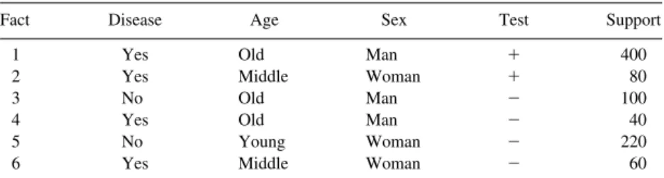
Table IV. Decision table.
Fact Disease Age Sex Test Support
1 Yes Old Man ⫹ 400
2 Yes Middle Woman ⫹ 80
3 No Old Man ⫺ 100
4 Yes Old Man ⫺ 40
5 No Young Woman ⫺ 220
6 Yes Middle Woman ⫺ 60
Table III. Certainty and coverage.
Rule Strength Certainty Coverage
1 0.00095 0.95 0.04500
2 0.01998 0.02 0.95500
3 0.00005 0.05 0.00005
4 0.97902 0.98 0.99995
● That 0.005% of persons with negative test results are suffering from the disease
● That 99.995% of persons with negative test results are not suffering from the disease
That means that if the test result is positive, it does not necessarily indicate the disease but negative test results most probably (almost for certain) do indicate lack of the disease. That is to say that the negative test result almost exactly identifies healthy patients.
For the remaining rules the accuracy is much smaller and, consequently, test results are not indicating the presence or absence of the disease. ■
Example 2. Now, let us consider a little more sophisticated example, shown in Table IV. Attributes disease, age, and sex are condition attributes, whereas test is the decision attribute.
The strength, certainty, and coverage factors for the decision table are shown in Table V. The flow graph for the decision table is presented in Fig. 1.
The following is a decision algorithm associated with Table IV: Table V. Certainty and coverage.
Fact Strength Certainty Coverage
1 0.44 0.92 0.83
2 0.09 0.56 0.17
3 0.11 1.00 0.24
4 0.04 0.08 0.09
5 0.24 1.00 0.52
6 0.07 0.44 0.15
(1) If (disease, yes) and (age, old) then (test,⫹) (2) If (disease, yes) and (age, middle) then (test,⫹) (3) If (disease, no) then (test,⫺)
(4) If (disease, yes) and (age, old) then (test,⫺) (5) If (disease, yes) and (age, middle) then (test,⫺)
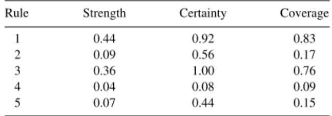
The certainty and coverage factors for the foregoing algorithm are given in Table VI. The flow graph for the decision algorithm is presented in Fig. 2.
The certainty factors of the decision rules lead to the following conclusions:
● Ninety-two percent of ill and old patients have positive test results
● Fifty-six percent of ill and middle-aged patients have positive test results
● All healthy patients have negative test results
● Eight percent of ill and old patients have negative test results
● Forty-four percent of ill and middle-aged patients have negative test results
In other words:
● Ill and old patients most probably have positive test results (probability⫽0.92)
● Ill and middle-aged patients most probably have positive test results (probability⫽0.56)
● Healthy patients have certainly negative test results (probability⫽1.00)
Table VI. Certainty and coverage factors.
Rule Strength Certainty Coverage
1 0.44 0.92 0.83
2 0.09 0.56 0.17
3 0.36 1.00 0.76
4 0.04 0.08 0.09
5 0.07 0.44 0.15
Figure 2. Flow graph for the decision algorithm.
Now let us examine the following inverse decision algorithm:
(1⬘) If (test,⫹) then (disease, yes) and (age, old) (2⬘) If (test,⫹) then (disease, yes) and (age, middle) (3⬘) If (test,⫺) then (disease, no)
(4⬘) If (test,⫺) then (disease, yes) and (age, old) (5⬘) If (test,⫺) then (disease, yes) and (age, middle)
Using the inverse decision algorithm and the coverage factor we get the following explanation of test results:
● Reasons for positive test results are most probably disease and old age (probability⫽ 0.83)
● Reason for negative test result is most probably lack of the disease (probability⫽0.76)
■ It is seen clearly from Examples 1 and 2 the difference between Bayesian data analysis and the rough set approach. In the Bayesian inference, the data are used to update prior knowledge (probability) into a posterior probability, whereas rough sets are used to understand what the data tell us.
8. CONCLUSION
Bayesian inference consists in updating subjective prior probabilities by means of data to posterior probabilities.
In the rough set approach, Bayes’ theorem reveals data patterns, used next to draw conclusions from data, in the form of decision rules, which refer to objective probabilities computed from data. Furthermore, the proposed approach enables us to apply Bayes’ theorem to give reasons for decisions by using reversed decision rules. Moreover, the association of flow graphs with decision tables gives new dimension to decision process analysis.
Acknowledgments The authors thank anonymous referees for critical comments.
References
1. Pawlak Z. Logic, probability, and rough sets. In: Karhumaki J, Maurer H, Paun G, Rozenberg G, editors. Jewels are forever, contributions on theoretical computer science in honor of Arto Salomaa. Berlin: Springer-Verlag; 1999. pp 364 –373.
2. Łukasiewicz J. Die logishen Grundlagen der Wahrscheinilchkeitsrechnung. Krako´w, 1913. In: Borkowski L, editor. Jan Łukasiewicz—selected works. Amsterdam: North Holland Publishing Co.; Warsaw: Polish Scientific Publishers; 1970. pp 16 – 63.
3. Bayes T. An essay toward solving a problem in the doctrine of chances. Philos Trans R Soc 1763;53:370 – 418; Reprint Biometrika 1958;45:296 –315.
5. Berthold M, Hand DJ. Intelligent data analysis. An introduction. Berlin: Springer-Verlag; 1999.
6. Box GEP, Tiao GC. Bayesian inference in statistical analysis. New York: Wiley; 1992. 7. Adams EW. The logic of conditionals, an application of probability to deductive logic.
Dordrecht: D. Reidel Publishing Co.; 1975.
8. Pawlak Z. Rough sets, decision algorithms and Bayes’ theorem. Eur J Oper Res 2002; 136:181–189.
9. Pawlak Z, Skowron A. Rough membership functions. In: Yager R, Fedrizzi M, Kacprzyk J, editors. Advances in the Dempster-Shafer theory of evidence. New York: Wiley; 1994. pp 251–271.
10. Tsumoto S, Tanaka H. Discovery of functional components of proteins based on PRIM-EROSE and domain knowledge hierarchy. Soft Computing, San Jose, CA, 1995. pp 780 –785.
11. Polkowski L, Skowron A, editors. Rough sets in knowledge discovery; Heidelberg: Physica-Verlag; 1998. 1:1– 601; 2:1–576.
12. Ford LR, Fulkerson DR. Flows in networks. Princeton, NJ: Princeton University Press; 1962.