P/N 4000126-10 RevA
Quantity One
®
User Guide for Version 4.2.1
Windows and Macintosh
Bio-Rad Technical Service Department
Phone: (800) 424-6723, option 2, option 3 (510) 741-6576
Fax: (510) 741-5802
E-mail: [email protected] (U.S.)
[email protected] (International)
Notice:
No part of this publication may be reproduced or transmitted in any form or by any means, electronic or mechanical, including photocopy, recording, or any information storage or retrieval system, without permission in writing from Bio-Rad.
Quantity One is a registered trademark of Bio-Rad Laboratories. The Discovery Series is a trademark of Bio-Rad Laboratories. All other trademarks and registered trademarks are of their respective companies. WASTE text engine © 1993–1997 Marco Piovanelli
Limitations of Liability:
Bio-Rad is not responsible for the misinterpretation of results obtained by following the instructions in this guide. Whenever possible, you should contact the Technical Services Department at Bio-Rad to discuss your results. As with all scientific studies, we recommend that you repeat your experiment at least once before making any significant conclusions for presentation or publication.
Table of Contents
iii
1. Introduction ... 1-1
1.1. Overview of Quantity One ... 1-1 1.2. Digital Data and Signal Intensity ... 1-2 1.3. About Gel Quality ... 1-3 1.4. Steps Involved in Using Quantity One ... 1-3 1.5. Computer Requirements ... 1-5 1.6. Installing on a PC ... 1-7 1.7. Installing on a Macintosh ... 1-8 1.8. Starting the Program ... 1-9 1.9. Contacting Bio-Rad ... 1-17
2. General Operation ... 2-1
2.1. Graphical Interface ... 2-1 2.2. Mouse-assignable Tools ... 2-6 2.3. Keyboard Commands ... 2-7 2.4. File Commands and Functions ... 2-7 2.5. Preferences ... 2-17 2.6. User Settings ... 2-23
3. Gel Doc ... 3-1
3.1. Gel Doc Acquisition Window ... 3-2 3.2. Step I. Position Gel ... 3-4 3.3. Step II. Acquire Image ... 3-5 3.4. Step III. Select Output ... 3-8 3.5. Image Mode ... 3-9 3.6. Exposure Status ... 3-10
3.7. Display ... 3-10 3.8. Options ... 3-12
4. Chemi Doc ... 4-1
4.1. Chemi Doc Acquisition Window ... 4-2 4.2. Step I. Position Gel ... 4-4 4.3. Step II. Acquire Image ... 4-5 4.4. Step III. Select Output ... 4-9 4.5. Image Mode ... 4-11 4.6. Exposure Status ... 4-12 4.7. Display ... 4-12 4.8. Options ... 4-14
5. GS-700 Imaging Densitometer ... 5-1
5.1. GS-700 Acquisition Window ... 5-2 5.2. Step I. Select Application ... 5-4 5.3. Step II. Select Scan Area ... 5-6 5.4. Step III. Select Resolution ... 5-7 5.5. Acquire the Image ... 5-9 5.6. Calibration ... 5-10 5.7. Other Options ... 5-14
6. GS-710 Imaging Densitometer ... 6-1
6.1. GS-710 Acquisition Window ... 6-2 6.2. Step I. Select Application ... 6-4 6.3. Step II. Select Scan Area ... 6-7 6.4. Step III. Select Resolution ... 6-8 6.5. Calibration ... 6-9 6.6. Acquire the Image ... 6-13 6.7. Other Options ... 6-14
Contents
v
7. GS-800 Imaging Densitometer ... 7-1
7.1. GS-800 Acquisition Window ... 7-2 7.2. Step I. Select Application ... 7-3 7.3. Step II. Select Scan Area ... 7-6 7.4. Step III. Select Resolution ... 7-7 7.5. Calibration ... 7-8 7.6. Acquire the Image ... 7-12 7.7. Other Options ... 7-12
8. Fluor-S MultiImager ... 8-1
8.1. Fluor-S Acquisition Window ... 8-2 8.2. Step I. Select Application ... 8-4 8.3. Step II. Position/Focus ... 8-6 8.4. Step III. Set Exposure Time ... 8-8 8.5. Acquire the Image ... 8-10 8.6. Options ... 8-11 8.7. Other Features ... 8-16
9. Fluor-S MAX MultiImager ... 9-1
9.1. Fluor-S MAX Acquisition Window ... 9-2 9.2. Step I. Select Application ... 9-4 9.3. Step II. Position/Focus ... 9-7 9.4. Step III. Set Exposure Time ... 9-8 9.5. Acquire the Image ... 9-10 9.6. Options ... 9-12 9.7. Other Features ... 9-17
10. Personal Molecular Imager FX ... 10-1
10.1. Personal FX Acquisition Window ... 10-2 10.2. Step I. Select Scan Area ... 10-4 10.3. Step II. Select Resolution ... 10-5
10.4. Acquire the Image ... 10-6 10.5. Options ... 10-7
11. Molecular Imager FX ... 11-1
11.1. FX Acquisition Window ... 11-2 11.2. Step I. Select Application ... 11-4 11.3. Step II. Select Scan Area ... 11-9 11.4. Step III. Select Resolution ... 11-10 11.5. Acquire the Image ... 11-11 11.6. Options ... 11-12
12. Viewing and Editing Images ... 12-1
12.1. Magnifying and Positioning Tools ... 12-1 12.2. Density Tools ... 12-5 12.3. Showing and Hiding Overlays ... 12-7 12.4. Multi-Channel Viewer ... 12-8 12.5. Image Stack Tool ... 12-10 12.6. Colors ... 12-12 12.7. Transform ... 12-15 12.8. Resizing and Reorienting Images ... 12-21 12.9. Subtracting Background from Entire Images ... 12-26 12.10. Filtering Images ... 12-31 12.11. Invert Data ... 12-36 12.12. Text Overlays ... 12-37 12.13. Erasing All Analysis from an Image ... 12-40 12.14. Sort and Recalculate ... 12-40
13. Lanes ... 13-1
13.1. Defining Lanes ... 13-1 13.2. Lane-Based Background Subtraction ... 13-10 13.3. Compare Lanes ... 13-13 13.4. Lane-based Arrays ... 13-17
Contents
vii
14. Bands ... 14-1
14.1. How Bands Are Identified and Quantified ... 14-2 14.2. Automatically Identifying All Bands ... 14-3 14.3. Identifying and Editing Individual Bands ... 14-10 14.4. Plotting Traces of Bands ... 14-14 14.5. Band Attributes ... 14-15 14.6. Displaying Band Information ... 14-18 14.7. Gauss-Modeling Bands ... 14-21 14.8. Irregularly Shaped Bands in Lanes ... 14-25
15. Standards and Band Matching ... 15-1
15.1. Defining and Applying Standards ... 15-2 15.2. Band Matching ... 15-13 15.3. Quantity Standards ... 15-23
16. Volume Tools ... 16-1
16.1. Creating a Volume Object ... 16-1 16.2. Moving, Copying, and Deleting Volumes ... 16-6 16.3. Volume Standards ... 16-7 16.4. Volume Background Subtraction ... 16-9 16.5. Volume Arrays ... 16-11
17. Colony Counting ... 17-1
17.1. Defining the Counting Region ... 17-2 17.2. Counting the Colonies ... 17-4 17.3. Displaying the Results ... 17-5 17.4. Making and Erasing Individual Colonies ... 17-6 17.5. Using the Histogram to Distinguish Colonies ... 17-6 17.6. Ignoring a Region of the Dish ... 17-8 17.7. Saving/Resetting Your Count ... 17-10 17.8. Saving to a Spreadsheet ... 17-10
18. Differential Display and VNTRs ... 18-1
18.1. Differential Display ... 18-1 18.2. Variable Number Tandem Repeats ... 18-4
19. Reports ... 19-1
19.1. The Report Window ... 19-1 19.2. Lane and Match Reports ... 19-5 19.3. 1-D Analysis Report ... 19-7 19.4. Similarity Comparison Reports ... 19-8 19.5. Volume Analysis Report ... 19-19 19.6. Volume Regression Curve ... 19-22 19.7. VNTR Report ... 19-24
20. Printing and Exporting ... 20-1
20.1. Printing ... 20-1 20.2. Exporting an Image in TIFF Format ... 20-5
Appendix A. Cross-Platform File Exchange ... A-1
Appendix B. Other Features ... B-1
ix
Preface
1. About This Document
This user guide is designed to be used as a reference in your everyday use of Quantity One®. It provides detailed information about the tools and
commands of Quantity One for the Windows and Macintosh platforms. Any platform differences in procedures and commands are noted in the text. This guide assumes you have a working knowledge of your computer operating system and its conventions, including how to use a mouse and standard menus and commands, and how to open, save, and close files. For help with any of these techniques, see the documentation that came with your computer.
This guide uses certain text conventions to describe specific commands and functions.
Some of the illustrations of menus and dialog boxes found in this manual are taken from the Windows version of the software, and some are taken from the
Example Indicates
File > Open Choosing the Open command under the File menu.
Dragging Positioning the cursor on an object and holding down the left mouse button while you move the mouse.
CTRL+S Holding down the Control key while typing the
letter s. Right-click/
Left-click/ Double-click
Clicking the right mouse button/ Clicking the left mouse button/ Clicking the left mouse button twice.
Macintosh version. Both versions of a menu or dialog box will be shown only when there is a significant difference between the two.
2. Bio-Rad Listens
The staff at Bio-Rad are receptive to your suggestions. Many of the new features and enhancements in this version of Quantity One are a direct result of conversations with our customers. Please let us know what you would like to see in the next version of Quantity One by faxing, calling, or e-mailing our Technical Services staff. You can also use Solobug (installed with Quantity One) to make software feature requests.
1-1
1. Introduction
1.1 Overview of Quantity One
Quantity One® is a powerful, flexible software package for imaging and analyzing 1-D electrophoresis gels, dot blots and other arrays, and colonies. The software runs in a Windows or Macintosh environment and has a graphical interface with standard pull-down menus, toolbars, and keyboard commands.
Quantity Onecan image and analyze a wide variety of biological data, including radioactive, chemiluminescent, fluorescent, and color-stained samples acquired from densitometers, phosphor imagers, fluorescent imagers, and gel documentation systems.
An image of a sample is captured using the controls in the imaging device window and displayed on your computer monitor. Image processing and analysis operations are performed using commands from the menus and toolbars.
Images can be magnified, annotated, rotated, and resized. They can be printed using standard and video printers.
All data in the image can be quickly and accurately quantitated using the Volume tools.
The lane-based functions can be used to calculate molecular weights, isoelectric points, VNTRs, Rf values, and other values. The software can measure total and average quantities, determine relative and actual amounts of protein, and count colonies in a Petri dish.
The software can cope with distortions in the shape of lanes and bands. Lanes can be adjusted along their lengths to compensate for any curvature or smiling of gels.
Data captured by the imaging device are stored in a file under a user-defined name. Files can be shared among all the Discovery Series™ software, or
images can be easily converted into TIFF format for compatibility with other Macintosh and Windows applications.
1.2 Digital Data and Signal Intensity
The Bio-Rad imaging devices supported by Quantity One are light and/or radiation detectors that convert signals from biological samples into digital data. Quantity One then displays the digital data on your computer screen, in the form of gray scale or color images.
A data object as displayed on the computer is composed of tiny individual screen pixels. Each pixel has an X and Y coordinate, and a value Z. The X and Y coordinates are the pixel’s horizontal and vertical positions on the image, and the Z value is the signal intensity of the pixel.
Fig. 1-1. Representation of the pixels in two digitally imaged bands in a gel.
For a data object to be visible and quantifiable, the intensity of its clustered pixels must be higher than the intensity of the pixels that make up the background of the image. The total intensity of a data object is the sum of the intensities of all the pixels that make up the object. The mean intensity of a data object is the total intensity divided by the number of pixels in the object. The units of signal intensity are Optical Density (O.D.) in the case of the GS-700 and GS-710 densitometers, the Gel Doc and Chemi Doc with a white
2-D View 3-D View
Introduction
1-3
light source, or the Fluor-S and Fluor-S MAX MultiImagers with white light illumination. Signal intensity is expressed in counts when using the Personal FX or FX, or in the case of the Gel Doc, Chemi Doc, Fluor-S, or Fluor-S MAX when using the UV light source.
1.3 About Gel Quality
Quantity One is very tolerant of an assortment of electrophoretic artifacts. Lanes need not be perfectly straight or parallel. Bands need not be perfectly resolved.
However, for accurate lane-based quantitation, we suggest that bands be reasonably flat and horizontal. Lane-based quantitation involves calculating the average intensity of pixels across the band width and integrating over the band height. For the automatic band finder to function optimally, bands should be well-resolved.
Dots that appear as halos, rings, or craters, or that are of unequal diameter, may be incorrectly quantified using the automatic functions.
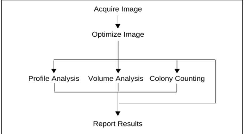
1.4 Steps Involved in Using Quantity One
Fig. 1-2. Steps Involved in Using Quantity One.
Acquire Image
Before you can use Quantity One to analyze a biological image, you need to capture the image into your computer. This may be done with one of the several Bio-Rad instruments supported by this software: the Molecular Imager FX and Personal Molecular Imager FX; the GS-700 and GS-710 Imaging Densitometers; the Gel Doc 1000/2000 and Chemi Doc gel documentation systems; and the Fluor-S and Fluor-S MAX MultiImagers. The resulting images are stored in files on your hard disk, network file server, or removable storage media.
Optimize Image
Once you have acquired an image of your sample, you may need to reduce any noise or background density caused by film fogging or the opacity of your carrier medium. A variety of functions exist to minimize background noise while maintaining data integrity.
Acquire Image
Optimize Image
Profile Analysis Volume Analysis Colony Counting
Introduction
1-5
Analyze Image
Once a “clean” image is available, you can use Quantity One to gather and analyze your data. In the case of 1-D gels, the software has tools for identifying lanes and defining, quantifying, and matching bands. Volume tools allow you to easily measure and compare the quantities of bands, spots, or arrays. The colony counting controls allow you to count the number of colonies in a Petri dish, as well as perform batch analysis.
Qualitative and quantitative data can be displayed in tabular and graphical formats.
Report Results
When your imaging and analysis are complete, you can print your results in the form of simple images, images with overlays, reports, tables, and graphs. You can export your images and data to other applications for further analysis.
1.5 Computer Requirements
This software will run on a PC as a Windows 98, NT 4.0, or 2000 application, or on a Macintosh PowerPC.
The amount of computer memory required for using the program is mainly determined by the file size of the images you will scan and analyze. Images scanned at high resolution can be quite large. For this reason, we recommend that you archive images on a network file server or removable storage media.
PC
The following are the minimum system requirements for installing and running on a PC:
Operating system: Windows 98, NT 4.0, or 2000. Processor: Pentium 166.
RAM: 64 MB for Gel Doc, Chemi Doc, and Fluor-S imaging systems. 128 MB for FX, Personal FX, and
densitometers.
Hard disk space: 3 GB. Recommended: Removable storage media (such as an Iomega Jaz drive) or a network file server. Monitor: 17" monitor, 1024 x 768 resolution, True Color (24- or
32-bit).
SCSI: Required for all Bio-Rad imaging devices except the Gel Doc and Chemi Doc. Adaptec SCSI card with EZ-SCSI software.
Printer: Optional.
Macintosh
Note: The default amount of memory assigned to this program on the
Macintosh is 64 MB. If the total RAM in your Macintosh is 64 MB or less (the minimum recommended amount is 128 MB), you should reduce the amount of memory assigned to the program to 10 MB less than your total RAM. With the application icon selected, go to File > Get Info in your Finder to reduce the memory requirements for the application. See your Macintosh computer documentation for details.
The following are the minimum system requirements for installing and running on a Macintosh:
Operating system: System 8.0 or higher. Processor/Model: PowerPC Macintosh 9500.
RAM: 64 MB for Gel Doc, Chemi Doc, and Fluor-S imaging systems. 128 MB for FX, Personal FX, and
densitometers.
Hard disk space: 3 GB. Recommended: Removable storage media (such as an Iomega Jaz drive) or network file server.
Monitor: 17" monitor, 1024 x 768 resolution, Millions of colors (24-bit).
Introduction
1-7
SCSI: Required to run all Bio-Rad imaging devices except the Gel Doc and Chemi Doc. Macintosh has built-in SCSI. Printer: Optional.
1.6 Installing on a PC
The software can be installed on a PC from a CD-ROM or you can download the installation program from the Internet. Make sure that Windows is up and running on your computer before attempting to install.
Note: Windows NT and 2000: You must be a member of the Administrators
group to install Discovery Series software on a computer. After
installation, members of the Users group must have "write" access to the Discovery Series folder to use the software.
Installing from a CD-ROM
Insert the Discovery Series™ CD-ROM into the CD-ROM drive on your computer. The installer will start automatically.
Downloading from the Internet
You can download the sofware from the Internet using Bio-Rad’s Web site. Go to www.discover.bio-rad.com, navigate to the Discovery Series download page, and select from the list of Windows applications to download. Follow the instructions to download the installer onto your computer. Then you can double-click on the Setup.exe icon on your desktop to begin running the installer.
Installed Files and Directories
The installation program will guide you through a series of screens. The installer will create a default directory tree under Program Files on your hard disk called Bio-Rad/The Discovery Series/Bin (you can select your own directory if you wish). The main program will be placed in the Bin directory. Additional directories for storing user profiles and sample images will also be created
The installer will place an application icon on your desktop and create a Discovery Series folder in the Programs folder on your Windows Start menu. Finally, after installation is complete, the installer will ask you if you want to start running the program.
1.7 Installing on a Macintosh
The software can be installed on a Macintosh from a CD-ROM or you can download the installation program from the Internet.
Installing from a CD-ROM
Insert the Discovery Series CD-ROM into the CD-ROM drive on your Macintosh. Double-click on the CD icon on your desktop, then double-click on the Install icon in the CD window.
Fig. 1-4. Installation program icon (Macintosh).
Downloading the Installation Program from the Internet
You can download the software from the Internet using Bio-Rad’s Web site. Go to www.discover.bio-rad.com, navigate to the Discovery Series download page, and select from the list of Macintosh applications to download. Follow
Introduction
1-9
the instructions to download the installer and place it on your desktop. Then you can double-click on the installer icon to begin running the installer.
Installed Files and Folders
The installer will guide you through a series of screens. The installer will create a folder on your hard drive that contains the main application and associated sample images (you can select a different folder if you wish). The installation will also create a folder called The Discovery Series in the Preferences folder in your System Folder; this contains the on-line Help and various system files.
Once installation is complete, the folder containing the application icon will appear open on your desktop.
1.8 Starting the Program
PC
The installation program creates an application icon on your desktop. To start the program, double-click on this icon.
The installer also creates a Discovery Series folder in the Programs folder on your Windows Start menu. You can start the program by selecting the application in this folder.
Fig. 1-5. Application icon.
Macintosh
After installation, the main application folder will be open on your desktop. To start the program, double-click on the application icon inside the folder.
1.8.a
Software License
When the program first opens, you should see a “Welcome” dialog box that shows the current status of your software license.
This program is protected by a software licensing system. You can have full use of the program for 30 days free of charge, after which you must purchase the software and obtain a password for continued use.
Most users will be able to start the program and begin the free trial period immediately after installation. If you open the software and see a “Free Trial” message, you can skip to section 1.8.c, Trial Period.
Unable to Obtain Authorization
If you attempt to start the program and receive an “Unable to obtain
authorization” message, you will need a hardware security key (HSK) to run the program. HSKs for both PC and Macintosh are included with the full CD-ROM package, or are available from Bio-Rad for downloaded software. If you receive this message, turn off your computer, attach the appropriate HSK as described in the following section, and restart the computer and program.
Note: Network License holders: Your network administrator is responsible for
the software license. If you have difficulty starting and running the program, contact your administrator.
1.8.b Attaching the Hardware Security Key
(If Necessary)
Before attaching the HSK, you should first attempt to start the software without the HSK. If the program opens successfully, you can skip this section.
Note: Some parallel port devices such as zip drives may be incompatible with
Introduction
1-11
PC
Fig. 1-6. PC Hardware Security Key
Before proceeding, please turn off your computer. If you have a printer attached to your computer’s parallel port, please turn that off as well.
The HSK attaches to the parallel port on the back of your PC. If a printer cable is attached to this port, disconnect it. After you have attached the HSK, you can attach the printer cable to the key itself and restart your computer and printer.
The code for the PC hardware security key is EYYCY. This is printed on the key itself.
You will also need to install the system driver that allows the computer to “read” the HSK.
Note: Windows NT and 2000 users must be in the local administrator group to
install the HSK driver.
To install the driver, click on your Windows Start menu and select Programs > The Discovery Series. Select Install HASP Hardware Security Key driver to begin installation.
Note: Windows 98 users must reboot their computer after installing the HSK.
Macintosh
Fig. 1-7. Macintosh Hardware Security Key
Before proceeding, please turn off your Macintosh.
The Macintosh HSK must be inserted in the Apple Desktop Bus (ADB) path. The ADB port is located on the back of your Macintosh.
Fig. 1-8. Apple Desktop Bus icon on back of Macintosh.
The HSK can be inserted at any point in the ADB path—between the computer and the keyboard, between the keyboard and the mouse, between the keyboard and the monitor, etc. After you have attached the HSK, you can restart your computer.
The code for the Macintosh HSK is QCDIY. This code is printed on the key itself.
1.8.c
Trial Period
When you start the program, the Software License screen will open. The type of screen you see will depend on whether you have an HSK, Network License, or neither.
Free Trial (No HSK or Network License)
If you do not have an HSK attached and do not have a Network License, the “Free Trial” screen will be displayed.
Introduction
1-13
Fig. 1-9. Free Trial screen.
Click on the Free Trial button. This will open the Software License Registration Form (see next section).
Temporary License (With HSK or Network License)
If you have an HSK attached or are using a Network License, the Software License screen will reflect the fact that you receive a 30-day temporary license (“Your license will expire on _______”).
Fig. 1-10. Temporary License screen.
Click on the Run button to begin using the software.
If you are using an HSK, some time during the 30-day license period, click on the Registration Form button to register your software. If your 30-day period has expired, a Free Trial button will appear when you open the software. Click on this button to open the Software License Registration Form and register your software.
If you are using a Network License, any time during the initial 30 days click on the Check License button. Your full Network License will be activated.
Note: Network License holders: If your Network License is not activated when
you click on Check License, notify your network administrator.
1.8.d Software Registration
Note: Network License holders do not need to register their software, and can
skip the following section.
To obtain a full individual software license, you will need to fill out in the information in the Software License Registration Form.
Introduction
1-15
Fig. 1-11. Software License Registration Form.
Note: If you do not yet have a Purchase Order Number or Software Serial
Number, you may leave these fields blank to receive a trial license.
Registering by Internet
If you have Internet access on your computer (the same computer on which you loaded the software), you can register quickly and easily.
In the Software License Registration Form, click on the Submit via Internet button.
Your information will be submitted automatically over the Internet, and a password will be generated automatically and sent back to your computer. Simply continue to run the application as before.
This password will be good for 30 days. During this period, if you have already submitted your Software Serial Number, click on Check License in the
Software License screen to update your license. (To access the Software License screen from within the application, select Help > Register.)
If you have not yet submitted your Software Serial Number, open the form again, enter the serial number, and resubmit it over the Internet. In 1–2 days, click on the Check License button to update your license.
Registering by Fax or E-mail
If you do not have Internet access, click on the Print button in the Software License Registration Form and fax the form to Bio-Rad at the number listed on the form. Alternatively, you can enter the contents of the form into an e-mail and send it to Bio-Rad at the address listed in the Registration Form. If you include your Software Serial Number in the form, Bio-Rad will contact you by fax or e-mail in 2–3 days with a full license.
If you do not include your Software Serial Number in the form, Bio-Rad will contact you in 2–3 days with a temporary 30-day license. Then, some time during the 30-day period, enter the serial number in the form and fax the revised form to Bio-Rad. Bio-Rad will contact you by fax or e-mail in 2–3 days with a full license.
Entering a Password
If you fax or e-mail your registration information, you will receive a password from Bio-Rad. You must enter this password manually.
To enter your password, click on Enter Password in the Software License screen. If you are not currently in the Software License screen, select Register from the Help menu.
Introduction
1-17
Fig. 1-12. Enter Password screen.
In the Enter Password screen, type in your password in the field. Once you have typed in the correct password, the OK light next to the password field will change to green and the Enter button will activate. Click on Enter to run the program.
1.9 Contacting Bio-Rad
Bio-Rad technical service hours are from 8:00 a.m. to 4:00 p.m., Pacific Standard Time in the U.S.
Phone: 800-424-6723, option 2, option 3 510-741-6576
Fax: 510-741-5802
E-mail: [email protected] (in the U.S.) [email protected] (International) For software registration, phone:
800-424-6723, option 1 (in the U.S.) 510-741-6996 (outside the U.S.)
2-1
2. General Operation
2.1 Graphical Interface
2.1.a
Menu Bar
Quantity One has a standard menu bar with pulldown menus that contain all the major features and functions available in the software.
Fig. 2-1. Menu bar.
• File—General file commands (Open, Save, Print), imaging device acquisition windows (Gel Doc, Chemi Doc, GS-700, GS-710, Fluor-S, Fluor-S MAX, Personal FX, FX).
• Edit—Text Overlay tools, Preferences, miscellaneous editing tools. • View—General viewing tools (Zoom Box, Grab), quick analysis tools
(Density in Box, Plot Density).
• Image—Transform function, image processing tools (Crop, Flip, Subtract Background), Invert Data.
• Lane—Lane-finding tools.
• Band—Band-finding and band-modeling tools. • Match—Standards, band matching tools. • Volume—Volume tools, array tools
• Analysis—Colony counting, Differential Display, VNTR analysis. • Reports—Analysis reports (Lanes, Matches, Volumes, VNTR),
Phylogenetic Tree, Similarity Matrix.
• Window—Tile windows commands, imitate zoom. • Help—Quick Guides, on-line Help, software registration.
Below the menu bar is the main toolbar, containing some of the most commonly used commands. Next to the main toolbar are the status boxes, which provide information about cursor selection and toolbar buttons.
2.1.b Main Toolbar
The main toolbar appears below the menu. It includes buttons for the main file commands (Open, Save, Print) and essential viewing tools (Zoom Box, Grab, etc.), as well as buttons that open the secondary toolbars and the most useful Quick Guides (Printing, Volumes, Molecular Weight, and Colony Counting).
Fig. 2-2. Main toolbar.
Tool Help
If you hold the cursor over a toolbar icon, the name of the command will pop up below the icon. This utility is called Tool Help. Tool Help appears on a time delay basis that can be specified in the Preferences dialog box under Edit > Preferences. You can also specify how long the Tool Help will remain displayed.
2.1.c
Status Boxes
There are two status boxes, which appear to the right of the main toolbar.
Fig. 2-3. Status boxes.
General Operation
2-3
The first box displays any function that is assigned to the mouse (see section 2.2, Mouse-assignable Tools). If you select a command such as Zoom Box, the name and icon of that command will appear in this status box and remain there until another mouse function is selected or the mouse is deassigned. The second status box is designed to supplement Tool Help (see above). It provides additional information about the toolbar buttons. If you hold your cursor over a button, a short explanation about that command will be displayed in this second status box.
2.1.d Secondary Toolbars
Secondary toolbars contain groups of related functions. You can open these toolbars from the main toolbar or from the View > Toolbars pulldown menu. These toolbars “float” over the application.
The secondary toolbars can be toggled between vertical, horizontal, and expanded formats by clicking on the resize button on the toolbar itself.
Fig. 2-4. Secondary toolbar formats and features.
The expanded toolbar format shows the name of each of the commands. Click on the “?” icon next to the name to display on-line Help for that command.
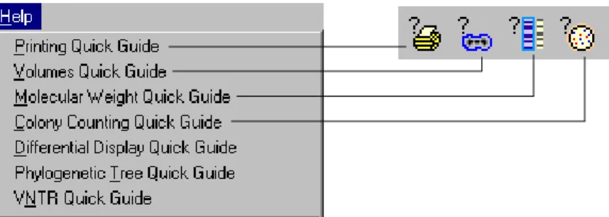
2.1.e Quick Guides
The Quick Guides are designed to guide you through the major applications of the software. They are listed under the Help menu; four of these are also available on the main toolbar.
Click on resize button Hold cursor over icon
Click on question marks for on-line help
to toggle format Expanded format
to reveal Tool Help
General Operation
2-5
Fig. 2-5. Quick Guides listed on Help menu and main toolbar.
The Quick Guides are similar in design to the secondary toolbars, but are application-specific.
Each Quick Guide contains all of the functions necessary for a particular application, from opening the image to outputting data.
Fig. 2-6. Example of a Quick Guide: Volumes
to indicate sequence for
Question marks open on-line Help
Key commands Toggle format
creating volumes, and outputting data preparing the image, Commands are numbered
Select Volumes Quick Guide from
Note: You will find that as you become more familiar with the application, you
will skip operations that are not needed for your particular images. In their expanded format, the Quick Guide commands are numbered as well as named, so that the order of operation is clear. Simply follow the steps and the Quick Guide will lead you through the analysis.
As with the secondary toolbars, you can click on the “?” next to the name of a function to display the Help text.
2.2 Mouse-assignable Tools
A number of commands don’t perform actions right away, but instead “assign” a function to your mouse (e.g., Zoom Box, Density at Cursor, Lane Background). You first select one of these tools from a menu or toolbar, then execute the command by clicking or dragging on the image.
Note: Mouse-assignable tools selected using the keyboard have slightly
different behavior. See the next section.
Fig. 2-7. Example of a mouse-assignable tool: Density at Cursor
When a “mouse-assignable” function is selected, the cursor appearance changes. The name and icon of the function appear in the status box next to the main toolbar (see section 2.1.c).
To deassign a function from the mouse, click on the toolbar button of the assigned function or click in the status box displaying the assigned function. You can also double-click on the Hide Overlays button.
General Operation
2-7
2.3 Keyboard Commands
Many commands and functions may be executed using keyboard commands (e.g., pressing the F1 key will activate the View Entire Image command). A list of key combinations and their associated commands will be displayed if you select Keyboard Layout from the Help menu.
The pulldown menus also list the shortcut keys for the menu commands.
Note: Mouse-assignable commands (see above) behave differently if you assign
them using the keyboard versus selecting them from the menus or toolbars. For example, to use the Zoom Box command as a keyboard command, position your cursor on the image where you want to begin to create the magnifying box, then press the F2 key. The command is assigned to your mouse and immediately activated, so that when you move your cursor over the image, the zoom box is created. When you click the mouse button once, the defined region is magnified and the tool is automatically deassigned from your mouse.
2.4 File Commands and Functions
This section describes the basic file commands and functions. These are selected from the File menu.
Fig. 2-8. File menu.
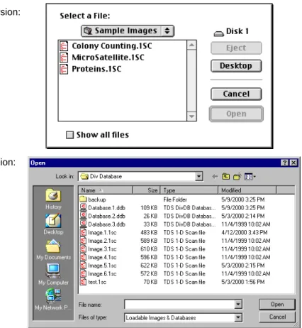
Open
To open a previously saved image, select Open from the File menu or main toolbar. This opens the Open dialog box.
General Operation
2-9
Fig. 2-9. Open dialog box.
In the dialog box, open a file by selecting the file name and clicking on the Open button. To look for files in other directories, use the directory pulldown menu at the top of the dialog box.
An image created in the Windows version of Quantity One can be opened in the Macintosh version, and visa versa. However, you must add a .1sc extension to your Macintosh files to open them in Windows.
Note: This version of Quantity One will open any image created with an earlier
version of Quantity One.
Macintosh version:
You can also open images captured by other Discovery Series software and Multi-Analyst™ software.
The application comes with a selection of sample images. In Windows, these may be found in the Discovery Series/Sample Images/1D directory. On the Macintosh, they are stored in the Sample Images folder in the Quantity One folder.
Opening TIFF Images
The Open command can also be used to import TIFF images from other software applications.
There are many types of TIFF formats that exist on the market. Not all are supported by the Discovery Series. There are two broad categories of TIFF files that are supported:
1. 8-bit Grayscale. Most scanners have an option between line art, full color, and grayscale formats. Select grayscale for use with the Discovery Series software. In a grayscale format, each pixel is assigned a value from 0 to 255, with each value corresponding to a particular shade of gray. 2. 16-bit Grayscale. Bio-Rad’s Molecular Imager (storage phosphor) and
Fluor-S imaging systems use 16-bit pixel values to describe intensity of scale. Molecular Dynamics™ and Fuji™ imagers also use 16-bit pixel
values. The Discovery Series understands these formats and can interpret images from both Bio-Rad and Molecular Dynamics storage phosphor systems.
Note: The program can import 8- and 16-bit TIFF images from both Macintosh
and PC platforms.
TIFF files that are not supported include:
1. 1-bit Line Art. This format is generally used for scanning text for optical character recognition or line drawings. Each pixel in an image is read as either black or white. Because the software needs to read continuous gradations to perform gel analysis, this on-off pixel format is not used. 2. 24-bit Full Color or 256 Indexed Color. These formats are frequently used
General Operation
2-11
Discovery Series, although most scanners that are capable of producing 24-bit and indexed color images will be able to produce grayscale scans as well.
3. Compressed Files. The software does not read compressed TIFF images. Since most programs offer compression as a selectable option, files intended for compatibility with the Discovery Series should be formatted with the compression option turned off.
Close
To close an image or scan, select File > Close. If the file has changed since it was last saved, a message box will ask you if you want to save the changes before closing.
Close All
File > Close All closes all open images. If you have made changes to any of the images, a message box will open for each unsaved image giving you the option of saving those changes.
Save
File > Save will save a new image or an old image to which you have made changes.
In Windows, new images will be given a .1sc extension when they are first saved.
Save As
File > Save As can be used to save a new image, rename an old image, or save a copy of a image in a different directory.
In Windows, new images will be given a .1sc extension when they are first saved.
Save All
Save All on the main toolbar or File menu saves all images that are currently open.
In Windows, new images will be given a .1sc extension when they are first saved.
Revert to Saved
File > Revert to Saved will reload the last saved version of the image you are working on. This is a quick way to undo any alterations you may have made to an image since you last saved it.
Any changes you have made since last saving the file will be lost. (Also, all open dialog boxes will be closed.) A message box will warn you before completing the command.
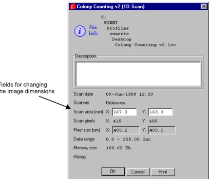
Image Info
File > Image Info displays general information about your image, including the scan date, scan area, number of pixels in the scan, data range, and the size of the scan file. There is also a field where you can type in a file description or comments.
General Operation
2-13
Fig. 2-10. Image Info box.
To print the file info, click on the Print button in the dialog box.
Change the Image Dimensions
You can change the dimensions of certain images using the Image Info dialog box.
Note: This feature is only available for images captured by a camera (such as
the Gel Doc or Fluor-S) or imported TIF images in which the dimensions are not already specified.
When you select File > Image Info for these types of images, the Image Info dialog box will include fields for changing the image dimensions.
Fig. 2-11. Image Info dialog box with fields for changing the image dimensions.
Enter the new image dimensions (in millimeters) in the appropriate fields. Note that the pixel size in the image ( in micrometers) will change to retain the same number of pixels in the image.
Reduce File Size
Image files can be quite large, and computer systems do not have unlimited memory or storage space. If you are having difficulty loading or storing a particular image, you may want to reduce the size of the file by reducing the number of pixels in the image. (You can also trim unneeded parts of an image to reduce its memory size. See section 12.8.a, Cropping Images.)
This function is comparable to scanning at a lower resolution, in that you are increasing the size of the pixels in the image, thereby reducing the total number of pixels and thus memory size.
Fields for changing the image dimensions
General Operation
2-15
Note: Reducing the file size of an image will result in some loss of resolution. In
most cases this will not affect quantitation. In general, as long as the pixel size remains less than 10 percent of the size of the objects in your image, changing the pixel size will not affect quantitation.
Select File > Reduce File Size to open the Reduce File Size dialog box.
The Reduce File Size dialog box shows you the size of the pixels in the image (Pixel Size: X by Y microns), the number of pixels in the image (Pixel Count: X by Y pixels), and the memory size of the image.
As you increase the size of the pixels, the pixel count will decrease, as will the memory size. You can increase the pixel size in either dimension (see the following figure for an example).
Fig. 2-12. Reduce File Size dialog box, before and after pixel size increase.
Pixel size in the “x” dimension increased
Pixel Count and Memory Size reduced Before:
Note: Since with most 1-D gels you are more concerned with resolving bands in
the vertical direction than the horizontal direction, you may want to reduce the file size by making rectangular pixels. That is, keeping the pixel size in the “y” dimension the same, while increasing the size in the “x” dimension. This lets you decrease the total number of pixels and therefore file size without sacrificing detail.
When you are finished, click on the OK button.
A pop-up box will give you the option of reducing the file size of the
displayed image or making a copy of the image and then reducing the copy’s size.
Reducing the file size is an irreversible process. For that reason, we suggest you make a copy of the image and reduce its file size. That way, if you lose too much resolution, you can simply delete the copy and try again. Once you are happy with the reduced image, don’t forget to delete the original. The goal is to save space!
Fig. 2-13. Confirm Reduce File Size pop-up box.
If you choose to make a copy of the image, you will be asked to enter a name for the new copy before the operation is performed.
Imaging Device Acquisition Windows
The File menu contains a list of Bio-Rad imaging devices supported by the Discovery Series software. These are:
General Operation
2-17
1. Gel Doc 1000/2000 2. Chemi Doc
3. GS-700 Imaging Densitometer 4. GS-710 Imaging Densitometer 5. Fluor-S MultiImager
6. Fluor-S MAX MultiImager 7. Personal Molecular Imager FX 8. Molecular Imager FX
Selecting a name in the File menu will open the acquisition window that allows you to scan using that instrument.
See the individual chapters on the imaging devices for more details.
Exit
File > Exit quits the application. You will be prompted to save any open files that have been changed.
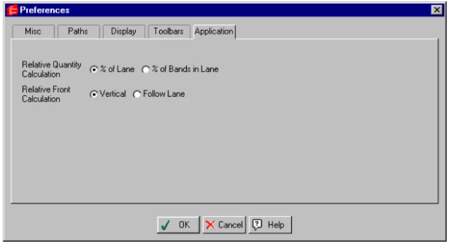
2.5 Preferences
The Preferences dialog box (accessed under the Edit menu) allows you to customize basic features of your system, such as displays and toolbars.
Fig. 2-14. Preferences dialog box.
Click on the appropriate tab to access groups of related preferences. After you have selected your preferences, click on OK to implement them.
2.5.a
Misc.
Click on the Misc tab to access the following preferences.
Memory Allowance
The Memory Allowance field allows you to specify the amount of virtual memory allocated for the application at start up. The default value of 512 megabytes is recommended. If you receive a warning message when opening the program that the amount of virtual memory is set too high, you can enter a smaller value in this field. However, this should be considered a temporary fix.
Institute Name
General Operation
2-19
GLP/GMP Mode
The GLP/GMP Mode checkbox allows you to prevent changes to an image that would change the raw image data. In GLP/GMP mode, the software will not allow the following operations to be performed:
• Reduce File Size (File menu) • Subtract Background (Image menu) • Custom Rotation (Image menu) • Noise filtering (Image menu) • Invert Data (Image menu)
If a user attempts to use any of these functions in GLP/GMP mode, he will receive a message that the function is not available.
To set GLP/GMP mode, click on the checkbox. A dialog box will pop up asking you to enter a password.
After you enter a password and click on OK, another dialog will ask you to reenter the password for confirmation. Retype the password and click on OK again.
To disable GLP/GMP mode, click on the checkbox to deselect it. The dialog box will pop up asking you to enter the password. When you click on OK, GLP/GMP Mode will be disabled.
Start Maximized
In the Windows version, the Start Maximized checkbox determines whether the application occupies the entire computer screen when first opened. If this is unchecked, the menu and status bars will appear across the top of the screen and any toolbars will appear “floating” on the screen.
2.5.b Toolbar
Click on the Toolbar tab to access the following preferences, which determine the behavior and positioning of the secondary toolbars and Quick Guides.
Show Volumes Quick Guide
If this checkbox is selected, the Volumes Quick Guide will open automatically when you open the program.
Align Quick Guide with Document
If this checkbox is selected, the Quick Guides will open flush with the edge of your documents. Otherwise, they will appear flush with the edge of the screen.
Quick Guide Placement and Toolbar Placement
These checkboxes determine which side of the screen the Quick Guides and toolbars will first open—left or right.
Placement Behavior
This setting determines whether a Quick Guide or toolbar will always pop up in the same place and format (Always Auto), or whether they will pop up in the last location they were moved to and the last format selected (Save Prior).
Toolbar Orientation
These option buttons specify whether toolbars will first appear in a vertical, horizontal, or expanded format when you open the program.
Guides Always on Top
If this checkbox is selected, Quick Guides will always float on top of images, and never be obscured by them.
Tool Help Delay and Persistence
Tool Help Delay allows you to specify the amount of time (in seconds) the cursor must remain over a toolbar icon before the Tool Help appears. First-time users may want to specify a short delay to learn the names of the toolbar
General Operation
2-21
functions, while experienced users can specify a longer delay once they are familiar with the icons.
Tool Help Persistence determines how long the Tool Help will linger on the screen after you move the cursor off a toolbar icon.
2.5.c
Application
Click on the Application tab to access the following preferences.
Relative Quantity Calculation
The Relative Quantity Calculation option allows you to define how the quantities of defined bands in lanes will be determined for all reports, histograms, and band information functions: either as a percentage of the signal intensity of an entire lane or as a percentage of the signal intensity of the defined bands in a lane.
Selecting % of Lane means that the total intensity in the lane (including bands and the intensity between bands) will equal 100 percent and the band that you select will be reported as a fraction thereof.
Selecting % of Bands in Lane means that the sum of the intensity of the defined bands in a lane will equal 100 percent, and your band will be reported as a fraction of that sum.
If you create, adjust, or remove bands with Relative Quantity defined as % of Bands in Lane, the relative quantities of all the other bands in the lane will update to reflect changes in the total intensity of defined bands.
Relative Front Calculation
The Relative Front Calculation option lets you select the method for
calculating the relative positions of bands in lanes . This affects the calculation of both Relative Front and Normalized Rf values.
1. Dividing the distance a band has traveled down a lane by the length of the lane (Follow Lane). This is useful if your gel image is curved or slanted.
2. Dividing the vertical distance a band has traveled from the top of a lane by the vertical distance from the top of the lane to the bottom (Vertical Projection).
Note: “Lane” and “band” refer here to lanes and bands as you have defined
them on your image. The top of a lane refers to the beginning of the lane line that you draw on the image, not necessarily the actual gel lane. If a lane is straight and vertical, these methods will give identical results. However, the results will differ if a lane is curved or slanted. Choose your preferred method by clicking on one of the two buttons next to the Relative Front Calculation prompt.
2.5.d Display
Click on the Display tab to access the following preferences.
Zoom %
The Zoom % field allows you to specify the percentage by which an image zooms in or out when you use the Zoom In and Zoom Out functions. This percentage is based on the size of the image.
Pan %
Pan % determines the percentage by which the image moves side to side or up and down when you use the arrow keys. This percentage is based on the size of the image.
Jump Cursor on Alert (Windows only)
When an alert box pops up in the Windows version of the application, you can set your cursor to automatically go to the OK button in the box by selecting Jump Cursor on Alert.
General Operation
2-23
Band Style
Bands in your gel image can be marked with brackets that define the top and bottom boundaries of the band, or they can be marked with a dash at the center of the band. Indicate your preference by clicking on the Brackets or Lines button next to the Band Style prompt. (This setting can be temporarily changed in the Band Attributes dialog box. However, all newly opened images will use the preferences setting.)
2.5.e Paths
Click on the Paths tab to access the following preference.
Temporary File Location
Temporary image files are normally stored in the TMP directory of your Discovery Series folder. The full path is listed in the field. To change the location of your temporary files, click on Browse and select a new directory. To return to the default TMP directory, click on the Default checkbox.
2.6 User Settings
If Quantity One is on a workstation that has multiple users, each user can have his or her own set of preferences and settings.
In multiple-user situations, the preferences and settings are associated with individual user names. On a PC with Windows 95/98/NT, your user name is the name you use to log onto the computer. On a Macintosh, your user name is the Owner Name under the File Sharing control panel.
Note: If you do not log onto your PC under Windows 95/98 or do not have a
Owner Name on your Macintosh, then you do not have a user name and your preferences and settings will be saved in a generic file.
3-1
3. Gel Doc
Fig. 3-1. Gel Doc.
Before you can begin acquiring images, the Gel Doc system must be properly installed and connected with the host computer. See the Gel Doc hardware manual for installation, startup, and operating instructions.
To use the Gel Doc, you will need to have the Bio-Rad-supplied acquisition board installed in your PC or Macintosh. The drivers for this board will be installed when you install the main software application.
Make sure that your Gel Doc camera is turned on. If the camera is not turned on, the Gel Doc acquisition window will open but the screen will be black, and you will be unable to Video Print.
Simulation Mode
Any of the imaging device acquisition windows can be opened in “simulation mode.” In this mode, an acquisition window will open and the controls will appear active, but instead of capturing real images, the window will create “dummy” images of manufactured data.
You do not need to be connected to an imaging device to open a simulated acquisition window. This is useful for demonstration purposes or practice scans.
To enter simulation mode, hold down the CTRL key and select the name of the
device from the File menu. The title of the acquisition window will indicate that it is simulated.
3.1 Gel Doc Acquisition Window
To acquire images using the Gel Doc, go to the File menu and select Gel Doc.... The acquisition window for the instrument will open, displaying a control panel and a video display window.
Gel Doc
3-3
Fig. 3-2. Gel Doc acquisition window
The Gel Doc video display window will open in “live” mode, giving you a live video display of your sample. If no image is visible, make sure the camera is on, check the cable connections, make sure the f-stop on the camera is not closed, and make sure that the protective cap is off the camera lens. Also check to see that the transilluminator is on and working.
The control panel has been arranged from top to bottom to guide you through the acquisition procedure. There are three basic steps to acquiring an image using the Gel Doc:
1. Position and focus the gel or other object to be imaged. 2. Acquire the image.
3. Select the output.
3.2 Step I. Position Gel
The Gel Doc window will open in “live” mode, giving you a live video display of your sample. In this mode, the Live/Focus button will appear selected, and frames will be captured and displayed at about 10 frames per second, depending on the speed of your computer.
You can use live mode to zoom, focus, and adjust the aperture on the camera, while positioning the sample within the area.
Note: Newer versions of the Gel Doc feature a motorized zoom lens that can be
controlled directly from the acquisition window using the Iris, Zoom, and Focus arrow buttons. Click on the Up/Down buttons while viewing your sample in the window to adjust the lens. These buttons will not be visible if you are connected to older versions of the Gel Doc without the
motorized zoom lens.
Fig. 3-3. Newer Gel Docs feature camera control buttons in the acquisition window.
You can also select the Show Alignment Grid checkbox to facilitate positioning.
The image should stay in focus while zooming. If focus is not maintained, refer to your Gel Doc hardware manual.
Note: After positioning your sample, you should check the Imaging Area
Gel Doc
3-5
the size of the area you are focusing on. To determine the size of the area you are focusing on, you can place a ruler in the Gel Doc box so that it is visible by the camera.
3.3 Step II. Acquire Image
For many white light applications, you can skip this step and save and print images directly from Live/Focus mode.
For UV light, chemiluminescent applications, or faint samples, you can take an automatic exposure based on the number of saturated pixels in the image or you can enter a specific exposure time.
Note: “Exposure” refers to the integration of the image on the camera CCD over
a period of time. The effect is analogous to exposing photographic film to light over a period of time.
Auto Expose
Auto Expose will take an exposure whose time length is determined by the number of saturated pixels in the image. This is useful if you are uncertain of the optimal exposure length.
Note: If you know the approximate exposure time you want (± 3 seconds), you
can skip this step and go directly to Manual Expose.
Click on the Auto Expose button to cancel Live/Focus mode and begin an automatic exposure. The Auto Expose button will appear selected throughout the exposure.
During the auto exposure, the image is continuously integrated on the camera CCD until it reaches a certain percentage of saturated pixels. This percentage is set in the Options dialog box. (Default = 0.75 percent. See Options below.)
Fig. 3-4. Auto Expose.
Once an image has reached the specified percent of saturated pixels, it is captured and displayed in the video display window, Auto Expose is automatically deactivated, the exposure time appears active in the Exposure Time field, and Manual Expose is activated.
Note: If you are having difficulty auto-exposing your sample, you can use
Manual Expose to adjust your exposure time directly. Most non-chemi applications only require an exposure time of a few seconds, which can be quickly adjusted using Manual Expose.
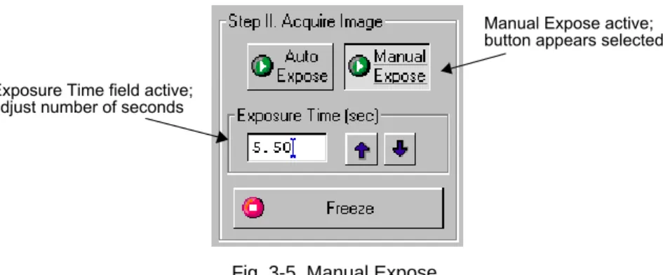
Manual Expose
If you know the approximate exposure time you want, you can click on the Manual Expose button. Manual Expose is automatically activated after Auto Expose has deactivated.
Click on Auto Expose; button appears depressed Can see Exposure Time automatically changing
Gel Doc
3-7
Fig. 3-5. Manual Expose.
With Manual Expose activated, you can adjust the exposure time directly by changing the number of seconds in the Exposure Time field. Type in a number or use the arrow buttons next to the field.
When the specified exposure time is reached, the last captured image will be displayed in the Gel Doc image window. The camera continues to integrate the image on the CCD, updating the display whenever the specified number of seconds is reached.
Once you are satisfied with the quality of the displayed image, click on the Freeze button to stop the exposure process. The last full exposure will be displayed in the image window.
Fig. 3-6. Freezing the exposure.
Manual Expose active; button appears selected Exposure Time field active;
adjust number of seconds
Click on Freeze to stop the exposure process
Note: Freeze is automatically activated if you adjust any of the subsequent
controls (e.g., Video Print, Image Mode, Display controls, etc.).
3.4 Step III. Select Output
The Gel Doc window has several output options.
Fig. 3-7. Output options.
Video Print
Clicking on Video Print will automatically send the currently displayed frame (either live or integrated) to a video printer. You can add information about your image to the bottom of the printout by selecting the appropriate checkboxes in the Options dialog box. (See Options, below.)
Annotate
Clicking on Annotate will open a separate image window displaying the captured image. The default name for the image will include the date, time, and user (if known).
The Text Overlay toolbar will also pop up to allow you to annotate your image.
Gel Doc
3-9
The image will not be saved until you select Save or Save As from the File menu.
Analyze
Clicking on Analyze will open a separate image window displaying the captured image. The default name for the image will include the date, time, and user (if known).
You can then analyze the image using the menu and toolbar functions. The image will not be saved until you select Save or Save As from the File menu.
Save
Clicking on Save will open a separate image window displaying the captured image. A Save As dialog box will automatically open displaying the default file name for the image, which will include the date, time, and user (if known). You can then change the file name and storage directory.
You can also save your image as a TIFF image for export to other applications.
3.5 Image Mode
The Image Mode option buttons allow you to set the type and scale of your data.
UV
Select this mode for fluorescent and chemiluminescent samples. With this mode selected, the data will be measured in linear intensity units.
White Light
Select this mode for reflective and transmissive samples. With this mode selected, the data will be measured in uncalibrated optical density (uOD) units.
3.6 Exposure Status
The Exposure Status bar shows the progress of your exposure. If your exposure time is greater than 1 second, the status bar display will give you a graphical representation of the remaining time before exposure is complete. If the exposure time is less than 1 second, the status bar will not refresh itself for each exposure; it will remain at 100 percent.
3.7 Display
The Display controls are useful for quickly adjusting the appearance of your image for output to a video printer. Adjusting these controls will
automatically freeze the video display and allow you to alter the image within the Gel Doc window.
Fig. 3-8. Display controls.
These controls are similar to those in the Transform dialog box.
Note: The Display controls will only change the appearance of the image. They
Gel Doc
3-11
Highlight Saturated Pixels
When this box is checked, any saturated pixels in the image will appear highlighted in red in the scan window and in the pop-up image window. To view/hide saturated pixels in the pop-up image window, use the Image > Transform command.
Invert Display
This checkbox will switch light spots on a dark background to dark spots on a light background, and visa versa. This will only affect how the image is displayed on the screen, not the actual image data.
Auto-scale
Clicking on Auto-scale will adjust your displayed image automatically. The lightest part of the image will be set to the minimum intensity (e.g., white), and the darkest will be set to the maximum intensity (e.g., black). You can then “fine tune” the display using the High, Low, and Gamma sliders described below.
High/Low Sliders
If Auto-scale doesn’t give you the appearance you want, you can use the High and Low sliders to redraw the image yourself. Dragging the High slider handle to the left will make weak signals appear darker. Dragging the Low slider handle to the right will reduce background noise.
You can also type specific High and Low values in the text boxes next to the sliders. Clicking anywhere on the slider bars will move the sliders
incrementally.
Gamma Slider
Some images may be more effectively visualized if their data are mapped to the computer screen in a nonlinear fashion. Adjusting the Gamma slider handle changes the light and dark contrast nonlinearly.
Reset
Reset will return the image to its original, unmodified appearance.
3.8 Options
Click on the Options button to open the Options dialog box. Here you can specify certain settings for your Gel Doc system.
Fig. 3-9. Available options in the Gel Doc acquisition window.
Click on OK to implement any changes you make in this box. Clicking on Defaults restores the settings to the factory defaults.
Gel Doc
3-13
DAC Settings
Note: The default DAC settings are highly recommended and should be
changed with caution.
These sliders may be used to adjust the minimum and maximum voltage settings of your video capture board. The minimum slider defines the pixel value that will appear as white in the image, while the maximum slider defines the pixel value that will appear as black. The slider scale is 0–255, with the defaults set to 60 minimum and 130 maximum.
Imaging Area
These fields are used to specify the size of your imaging area in centimeters, which in turns determines the size of the pixels in your image (i.e.,
resolution). When you adjust one imaging area dimension, the other dimension will change to maintain the aspect ratio of the camera lens.
Note: Your imaging area settings must be correct if you want to do 1:1 printing.
These are also important if you are comparing the size of objects (e.g., using the Volume Tools) between images.
Auto Exposure Threshold
When you click on Auto Expose, the exposure time is determined by the percentage of saturated pixels you want in your image. This field allows you to specify that percentage.
Typically, you will want less than 1 percent of the pixels in your image saturated. Consequently, the default value for this field is 0.75 percent.
Reminder
When this checkbox is selected, the software will warn you to turn off your transilluminator light when you exit the Gel Doc acquisition window or when your system is “idle” for more than 5 minutes.
Note: If you are performing experiments that are longer than 5 minutes (e.g.,
Video Printing Footer Information
The checkboxes in this group allow you to specify the information that will appear at the bottom of your video printer printouts.
Save Options
To automatically create a backup copy of any scan you create, select the Make Backup Copy checkbox.
With this checkbox selected, when you save a scan, a backup copy will be placed in the same directory as the scanned image. Windows backup files will have an “.sbk” extension. Macintosh backup files will have the word
“backup” after the file name.
This backup copy will be read-only, which means that you cannot make changes to it. You can open it like a normal file, but you must save it under a different file name before editing the image or performing analysis.
4-1
4. Chemi Doc
Fig. 4-1. Chemi Doc.
Before you can begin acquiring images, the Chemi Doc system must be properly installed and connected with the host computer. See the Chemi Doc hardware manual for installation, startup, and operating instructions.
To use the Chemi Doc, you will need to have the Bio-Rad-supplied acquisition board installed in your PC or Macintosh. The drivers for this board will be installed when you install the main software application.