The Distributional Impact of Public Services When Needs Differ

DISCUSSION PAPER SERIES

Forschungsinstitut zur Zukunft der Arbeit Institute for the Study of Labor

The Distributional Impact of Public Services

When Needs Differ

IZA DP No. 4826

March 2010 Rolf Aaberge Manudeep Bhuller Audun Langørgen Magne Mogstad

The Distributional Impact of

Public Services When Needs Differ

Rolf Aaberge

Statistics Norway and IZA

Manudeep Bhuller

Statistics Norway

Audun Langørgen

Statistics Norway

Magne Mogstad

Statistics Norway and IZA

Discussion Paper No. 4826 March 2010

IZA

P.O. Box 7240 53072 Bonn

Germany

Phone: +49-228-3894-0 Fax: +49-228-3894-180

E-mail: [email protected]

Any opinions expressed here are those of the author(s) and not those of IZA. Research published in

this series may include views on policy, but the institute itself takes no institutional policy positions.

The Institute for the Study of Labor (IZA) in Bonn is a local and virtual international research center and a place of communication between science, politics and business. IZA is an independent nonprofit organization supported by Deutsche Post Foundation. The center is associated with the University of Bonn and offers a stimulating research environment through its international network, workshops and conferences, data service, project support, research visits and doctoral program. IZA engages in (i) original and internationally competitive research in all fields of labor economics, (ii) development of policy concepts, and (iii) dissemination of research results and concepts to the interested public.

IZA Discussion Papers often represent preliminary work and are circulated to encourage discussion. Citation of such a paper should account for its provisional character. A revised version may be available directly from the author.

IZA Discussion Paper No. 4826 March 2010

ABSTRACT

The Distributional Impact of Public Services When Needs Differ

*

Despite a broad consensus on the need to take into account the value of public services in distributional analysis, there is little reliable evidence on how the inclusion of such non-cash income actually affects poverty and inequality estimates. In particular, the equivalence scales applied to cash income are not necessarily appropriate when including non-cash income, because the receipt of public services is likely to be associated with particular needs. In this paper, we propose a theory-based framework designed to provide a coherent evaluation of the distributional impact of local public services. The valuation of public services, identification of target groups, allocation of expenditures to target groups, and adjustment for differences in needs are derived from a model of local government spending behaviour. Using Norwegian data from municipal accounts and administrative registers we find that the inclusion of non-cash income reduces income inequality by about 15 percent and poverty rates by almost one-third. However, adjusting for differences in needs for public services across population subgroups offsets about half the inequality reduction and some of the poverty decrease.

JEL Classification: D31, H72, I30

Keywords: income distribution, poverty, public services, non-cash income, needs adjustment, equivalence scales

Corresponding author: Rolf Aaberge

Research Department Statistics Norway P.O. Box 8131 Dep. N-0033 Oslo

Norway

E-mail: [email protected]

*

We would like to thank the Norwegian Research Council for financial support, Marit Østensen and Simen Pedersen for preparing the data, and Kathleen Short, Terje Skjerpen, and two anonymous referees for helpful suggestions and comments.

1 1. Introduction

Most studies of poverty and income inequality focus exclusively on cash income and omit the value of public services. Smeeding et al. (1993; p 230) suggest that this practice may be due to the fact that “the problems inherent in the measurement, valuation, and imputation of non-cash income to individual households on the basis of micro data files are formidable.” Nevertheless, the conventional focus on cash income yields an incomplete and perhaps misleading picture of the distribution of economic well-being, not least because about half of welfare state transfers in developed countries are in-kind benefits such as health insurance, education and other services (Garfinkel et al., 2006).

As the tax burden levied on households represent a deduction from their disposable income, it is important to account for the services which governments provide to households through these taxes. The omission of public services from the definition of income may call into question the validity of income comparisons across population subgroups, over time, and between countries. Furthermore, this omission can have important policy implications given the wide range of policies that aim to fight poverty and reduce inequality. For these reasons, the Canberra Group (Expert Group on Household Income Statistics, 2001) and Atkinson et al. (2002) have expressed the need for more research on the distributional impact of public services. Definition and measurement of public in-kind benefits require solutions of conceptual as well as practical problems, which have been raised and explored in a number of studies.1

While these studies represent a significant step forward, our aim is to further develop a framework for evaluating the distributional impact of public services.

Extended income. The term extended income denotes the sum of disposable cash income and

non-cash income, where non-cash income accounts for the value of local public services received by different individuals and households. The measurement of non-cash income involves three steps: Valuation, allocation, and adjustment for differences in needs through the use of equivalence scales. Our paper departs from the previous literature in that a model of

1_{See e.g. Smeeding (1977), Ruggles and O’Higgins (1981), Gemmell (1985), Smeeding et al. (1993), Evandrou et al. (1993),}

2

local government spending behaviour forms the basis for each step. This framework therefore provides a coherent framework for evaluating the distributional impact of public services.

Valuation and allocation. From a model of local government behaviour, we derive a linear

expenditure system that proves useful in explaining differences in spending of municipalities across sectors and between population subgroups. In particular, the allocation of public service expenditure to households is based on estimates of sector-specific minimum quantities assigned to different target groups. These estimates are identified from information on sector-specific expenditures and the demographic characteristics of the population in each municipality. The estimation of the model is based on detailed local government accounts and community characteristics for Norwegian municipalities.

In our main analysis, we follow the previous literature closely in valuating public services at the cost of their provision. However, we perform a sensitivity analysis in which the value of public services is adjusted by estimated price indices that account for variation in production costs across municipalities, in line with the suggestions of Aaberge and Langørgen (2006).

Needs adjustment. The importance of accounting for needs and economies of scale in

households’ in analyses of cash income distributions is universally acknowledged. As argued by Radner (1997), however, equivalence scales designed to account for needs and economies of scale in cash income are not necessarily appropriate when analyzing extended income. For instance, the elderly tend to utilize health services more often than younger people due to different health status, and children have a genuine need for education. As a consequence, studies using the equivalence scales designed for cash income risk overestimating the equivalent incomes of groups with relatively high needs for public services. A contribution of this paper is to relax the assumption that the relative needs of different subgroups remain unchanged when the definition of income changes.

To derive an equivalence scale for extended income, we use the minimum expenditures identified in the spending model of the local governments as a basis for assessing the relative needs for public services of different target groups. The justification of this approach is that the estimated minimum expenditures can be considered as a result of central government regulations, expert opinion, and/or a consensus among local governments about how much

3

spending the different target groups need, given the budget constraint that the municipalities face. The fact that the equivalence scale is based on the same model used to derive the allocation method does not imply that the allocated non-cash income is exactly offset by the needs of the different target groups. The reason is threefold. First, the recipients live in different municipalities which have different economic capacity to produce public services. Second, local governments have discretion in their spending across service sectors, as well as in spending priorities on different target groups. And third, since the needs-adjusted equivalence scale is defined as a weighted average of the scale for cash income and the scale for non-cash income, the needs adjustment is a function of both cash and non-cash income. This means that individuals who are equal with respect to needs for public services and who belong to the same municipality, are affected differently by the needs adjustment if their cash incomes differ.

The Norwegian case. Norway emerges as an interesting country for studying the distributional impact of local public services for reasons beyond data availability and quality. First of all, Norway is a relatively large country with a dispersed population and relatively large public sector where local governments play an important role in the provision of public services. In Norway, the central government has introduced an equalization program in the grant system for local governments. However, important income components such as income from hydroelectric power plants and regional development transfers are not accounted for in the equalization scheme. Moreover, there is variation in local government spending across service sectors, as well as in spending priorities on different target groups (Aaberge and Langørgen, 2003). Consequently, some municipalities may be more effective than others in fighting poverty and reducing inequality, either because they can provide a generally higher level of services or because they are targeting vulnerable groups.

Outline. Section 2 discusses the model of local government spending behaviour and the

methods used to valuate and allocate public services, before justifying the equivalence scales for non-cash income and extended income. Section 3 describes the empirical implementation of these methods and reports estimation results from the model of local government spending. Section 4 presents empirical results showing the impact of local public services on poverty and income inequality estimates, before Section 5 concludes.

4 2. Local public services

This section describes the model of local government spending behaviour, before presenting the methods used to valuate and allocate public services and derive the equivalence scales for non-cash income and extended income.

It should be noted that it is beyond the scope of this paper to evaluate the distributional impact of public services that are not provided by local governments, most notably central government administration and infrastructure, defence, police services, secondary and post-secondary education, and public hospitals. Though figuring out how to value, allocate, and needs adjust those services is important, it is left for future research.

2.1. Spending behaviour of local governments

As was demonstrated by Aaberge and Langørgen (2003), the linear expenditure system (LES) proves helpful in explaining differences in the spending behaviour of Norwegian municipalities, provided that account is taken for heterogeneity in expenditure needs and in local preferences for allocation of income to different services. To account for heterogeneity in preferences over service sectors and target groups of local governments, we use the following specification of a Stone-Geary utility function,

(2.1)

1 1

log ,

s k

ij ij ij

i j ij

x

V  



 

  

 _ _

 



where V is utility of the local government, and x_ij is the production of service i per person of target group j. The parameter ij is interpreted as the minimum quantity per person of service i targeted to group j and can also be considered as a measure of the local government’s assessment of the need for different services targeted to different population subgroups. The parameter ij is interpreted as the marginal budget share for spending on group j in service sector i.

When the local government is assumed to allocate resources both to different service sectors and to different target groups, the budget constraint can be specified as

5

(2.2)

1 1 1 1

,

s k s k

i ij j ij j

i j i j

y  x z u z

   



 





where y is total per capita income of the local government, _i is the cost per unit in the production of service i, z_j is the population share that belongs to target group j and u_ij _{i ij}x is the spending per person on service i for target group j. Thus, u z_{ij j} is spending of type i targeted to group j measured per person in the population. By maximizing utility in (2.1) subject to the budget constraint (2.2), we obtain the following linear expenditure system,

(2.3) 1 1

1 1

, 1,2,..., , 1,2,..., , 1,

s k ij j i ij j ij i ij j

i j s k

ij i j

u z   z  y   z i s j k

         _  _     





where 1 1 s k i ij j i j

y   z

 





is discretionary income, that is, the income remaining when the minimum expenditures have been covered. Minimum expenditure in sector i targeted to group j

is defined by  _{i ij j}z . Exclusion restrictions of the type _ij 0 capture the fact that each target group does not necessarily receive all services.

Since allocation of spending to target groups, u_ij, is normally not reported in accounting data we identify the parameters of the model by imposing the following multiplicative structure on the marginal budget shares,

(2.4)

1

1

, 1,2,..., , 1,2,..., , 1,

1, 1,2,..., , ij i ij

s i i k ij j

i s j k

i s             





where _i is the marginal budget share for service sector i, and _ij is the share of sector-specific discretionary income in service sector i that is allocated to target group j. Inserting (2.4) into (2.3) and aggregating across target groups within each service sector yield

6

(2.5)

1 1 1

, 1,2,..., ,

k s k

i i ij j i i ij j

j i j

u   z  y   z i s

  

 

  _  _ 

 



 

where ui 



k_j1u zij j is expenditure (per capita) in service sector i, which is reported in the

accounting data of the municipalities. The total per capita minimum quantity in sector i is defined by _i 



k_j1_{ij j}z . Thus, owing to the additive properties of the linear expenditure system, it is possible to estimate minimum quantities for different target groups and different service sectors. By allowing the minimum quantity parameters _ij to vary across target groups, we obtain a flexible modelling framework that accounts for different needs for public services across different demographic groups. We also allow the unit cost parameters _i and the marginal budget share parameters _i to vary with observed variables. However, for the purpose of identification we assume that certain variables affect unit costs but not minimum quantities. This assumption helps to clarify the distinction between unit costs and service needs of the population.2 Specifically, we introduce the following specification for the unit cost parameters:

(2.6) _{i i0} 1 _ih( _{h h}) , 1,2,..., , h

p p i s

  _    _ 







where p_h is a variable that affects unit costs in at least one of the service sectors and p_h is the national mean of variable p_h. For instance, we assume that settlement pattern and economies of scale affect unit costs, which means that small municipalities with a dispersed population are allowed to face different unit costs in service production compared to other municipalities. By contrast, the sector-specific minimum quantities (_i) depend on population shares of different target groups which capture the local need for services such as child care, education and care for the elderly.

Equation (2.6) is expressed in terms of variables measured as deviations from national average levels. Consequently, the parameter _i0 can be interpreted as the average price level in service

2 _{Aaberge and Langørgen (2003) used a different approach by replacing the minimum expenditure terms with linear functions}

7

sector i. Minimum quantities and unit costs are, however, only identified up to a multiplicative constant, since multiplying unit costs by a constant and dividing subsistence output by the same constant cannot be traced from the reduced form parameters of the model. Natural scales of measurement for output and unit costs of local public services are not available. However, since expenditures are defined by the product of output and unit costs an appropriate scale emerges by normalizing the average price levels to 1 (_i0 1,i1,2,...,s). This means that unit cost _i

is defined as a price index with the average for the entire country equal to 1. Moreover, it follows that service outputs are measured in money terms and are interpreted as monetary values of output for an average price level. Note, however, that the normalization of prices imposes no restrictions on the model other than a choice of measurement scale for prices and outputs.

Heterogeneity in marginal budget shares is due to different preferences across municipalities for allocating discretionary income to service sectors. Let

(2.7)

0

0 1

1

, ( 1,2,..., ), 1,

0 0,

i i ih h h s

i i

s ih i

t i s

for all h

  

  



   

 







where t_h is a taste variable that affects the preferences for allocating discretionary income. For instance, the party composition of the local government council may influence such service priorities. This specification allows for different political priorities over service sectors across local governments. Such priorities are assumed to affect the allocation of discretionary income to services sectors, whereas the minimum quantities are assumed to be determined by variation in local needs that are reflected in the relative size of different target groups.

2.2 Allocation method

As noted above, the allocation of spending to different services is reported in local government accounts. Yet the allocation of spending to target groups is not observed, reflecting data availability in most countries. This means that marginal budget share _ij for different target

8

groups are not identified. A feasible solution to this problem is to utilize the information captured by the minimum quantities _ij to determine the relative priority of different target groups. By assuming that the sector-specific discretionary income is allocated to target groups by the same proportions as minimum expenditures, that is,

(2.8)

1

, 1, 2,..., , 1, 2,..., , ij j

ij k ij j j

z

i s j k

z

 





  



the local government model is fully identified. Thus, the parameter _ij can be interpreted as the proportion of the minimum quantity (and minimum expenditure) in sector i received by target group j. Inserting (2.8), (2.4) and (2.5) in (2.3) gives the following allocation of spending to target groups

(2.9)

1

, 1, 2,..., , 1, 2,..., , ij j

ij j k i ij j j

z

u z u i s j k

z

 



  



which means that sector-specific spending is allocated to target groups by the same proportions as minimum quantities (and minimum expenditures). Note that the share of expenditure received by a target group is an increasing function of the target groups’s share of the population, as well as of the estimated minimum quantity per person in the target group. As is demonstrated by (2.9), estimates of the target-group-specific expenditures u_ij can be derived from estimates of the minimum quantities _ij, and from data on sector-specific expenditures and proportions of the population belonging to various target groups.

2.3 Equivalence scales

Equivalence scales play an important role in analysis of inequality and poverty as a means for achieving interpersonal comparability of cash income. Both the methods for deriving equivalence scales and the normative assumptions made by them are subject to considerable debate. While theoretically justified equivalence scales can be constructed from the cost functions for households with different demographic characteristics, most empirical analysis typically use more pragmatic scales adjusting crudely for differences in household size and composition (see e.g. Coulter et. al. 1992). In either case, the equivalence scales designed for cash income are not necessarily appropriate when analyzing extended income, because the

9

receipt of public services (like education for children and care for the elderly) are associated with particular needs.3 If we were to use the equivalence scales designed for cash income on extended income, we risk overestimating the equivalent extended income for individuals with high needs for public services.

To derive an equivalence scale for extended income, consider a social planner employing the minimum expenditures identified in the spending model of the local governments as a basis for assessing the relative needs of different target groups. The justification for this approach is that the estimated minimum expenditures can be considered as a result of central government regulations, expert opinion, or a consensus among local governments about how much spending the different target groups need, given the budget constraint that the municipalities face. Moreover, we assume that the social planner uses the same functional form for measuring individual well-being produced by public services as is used by local governments to decide the spending on public services.

However, while the marginal budget share parameters of the utility function (2.1) of the local governments allow for heterogeneity in spending across sectors as well as across target groups, the aim of the social planner is to employ a social evaluation framework that treats individuals symmetrically and independent of where they live after adjusting for relevant non-income heterogeneity. Thus, we replace the marginal budget share parameters _ij of the utility function (2.1) with parameters that solely depend on the group- and sector-specific minimum expenditures  _{i ij j}z . The following specification

(2.10)

0 1

, 0,1,..., , 1, 2,..., , i ij j

ij s k

i ij j i j

z

i s j k

z

  

 

 

  

 

appears particular attractive since it captures the needs structure exhibited by the minimum quantity parameters. Note that sector 0 is added as a composite good that includes consumption financed by the cash income, where _0j is the minimum quantity of cash income per person for target group j and ₀ represents the price index of private consumption. Next, by inserting (2.10) in (2.1) we get

3 _{For example, the equivalence scales estimated by Jones and O’Donnell (1995) and Zaidi and Burchardt (2005) imply that the}

10 (2.11) 0 1 log s k ij ij ij

i j ij

x

W  

       _ _  



_,

which will be considered as the evaluation function of the social planner. The cost function of the social planner is given by

(2.12)

01,02,..., _{0 1 0 1}

1 1

( , , ) min log .

sk

s k s k

i ij j ij ij i ij j s k

x x x

i j i j _{i j i ij j} ij

z x

C w x z w

z               _{  }      _ _      





 

 π z

where z( z ,z ,...,z )_{1 2 k} gives the relative distribution of the population on target groups. Thus, from the social planner’s point of view C w( , , )π z gives the minimum cost (per capita) to get welfare level w for a population characterized by k target groups. By solving the minimization problem (2.12) we find that the cost function Cadmits the following decomposition

(2.13)









0 1

, , w 1 s k

i ij j i j

C w e   z

 

 



π z .

Let C w_j( , )π be defined by

(2.14)









0

, w 1 s , 1, 2,...,

j i ij

i

C w e   j k



 





π .

Inserting (2.14) in (2.13) yields the following decomposition of the cost function

(2.15)









1

, , k _j , _j j

C w C w z







π z π .

Due to the Stone-Geary structure of the social evaluation function W defined by (2.11), it is straightforward to prove that C w_j( , )π can be considered as a separate cost function for a member of target group j. The cost function C_j shows how much money the social planner has

the distribution of extended income.

11

to spend on each person in target group j to ensure that the social welfare level wis attained for each member of target group j ( j1 2, ,...,k). Thus, the associated price-adjusted target group-specific equivalence scale NPA_j is defined by

(2.16)





 

0 0 0

0 0 0

,

, 1, 2,.., ,

s s s

i ij i ij ij

j i i i

j s s s

r

ir ij ir

i i i

C w

NPA j k

C w                













 

π 1 ,

where the reference target group r is a single adult below 67 years of age,4 and the (hypothetical) reference municipality is characterized by a price vector with all prices equal to 1. It follows from (2.16) that the equivalence scale NPA_j is independent of the income levels of the target groups.5 Note that the NPA_j accounts for needs for public services as well as for needs for cash income. Since

0 0

s s

j i ij ij

i i

   

 







can be interpreted as a target-group-specific price index and

0 0

s s

j ij ir

i i

NA  

 







as an average needs-adjusted equivalence scale, NPA_j

admits the following convenient decomposition

(2.17) NPA_j _jNA_j.

In the general case the equivalence scale depends on variation in the price level across municipalities. The reason for this is that residents in high-cost municipalities require higher spending to reach the same standard of living as residents in low-cost municipalities. To pin down the distributional impact of allowing for changes in the relative needs of subgroups when we move from cash to extended income, we assume that prices do not vary across municipalities, which means thatNPA_j NA_j. To assess the importance of allowing for variation in production costs, we will allow for differences in unit costs using the more general

j

NPA equivalence scale.

4 _{Moreover, the reference household is assumed not to possess any of the characteristics that trigger additional expenditure}

needs, such as unemployment, refugee status, divorce or poverty.

5 _{This structure, called independence of base utility, has previously been discussed by Lewbel (1989) and Blackorby and}

12

Another convenient decomposition property of the equivalence scale defined by (2.16) is given by (2.18) , ,..., 2 , 1 , , ,..., 2 , 1 , , , ,..., 2 , 1 , ) 1 ( 1 1 0 0 0 0 0 k j NC k j CI k j NC CI NPA s i ir s i i ij j r j j s i ir r r j r j r j         







             

where CI_j is the equivalence scale for cash income, NC_j is the scale for non-cash income, and r

 is the weight that is given to cash income in the combined NPA scale for extended income. While the NC scale is a function of the minimum expenditures identified in the spending model of local governments, we will follow the previous literature in using a pragmatic scale for CI. In our main results, we will apply the much used EU scale for cash income, but as a robustness check we employ the OECD scale instead. The combined NA scale (and NPA scale) requires assessment of the weight _r. The empirical implementation in Section 3.4 discusses two alternative methods for determining this parameter.

The equivalence scales in equations (2.17) and (2.18) can be defined both on individual and household level. As there are no clear-cut economies of scale in the consumption of public non-cash income, such as education and health care, the local public services are treated as private goods in the NC scale for public services. The NC scale on the household level is computed by summation of individual scales over all individuals that belong to a given household. The parameter _r in equation (2.18) does not differ across individuals or municipalities. Thus, the parameter is not affected by aggregation over households. Since the EU scale is defined on the household level, it can be weighted together with the NC scale aggregated to the household level, using the parameter _r as the weight for cash income. It follows that economies of scale in consumption are included in the NA scale (and NPA scale) to the degree that the equivalence scale for cash income (the EU scale) accounts for economies of scale. A comparison of the EU

13 3. Empirical implementation

This section describes the empirical implementation of the methods outlined above using Norwegian data. We also outline the methods used to evaluate the income distribution. Specifically, Section 3.1 describes the data and some definitional issues. Estimation results of the model for local government spending are given in Section 3.2. Section 3.3 describes how the value of public services is allocated to individuals. Section 3.4 defines equivalent income measures that are utilized in the analysis of income distribution. Inequality measures and poverty thresholds are defined in Section 3.5.

3.1 Data

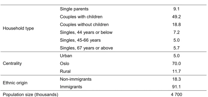
Population of study. Our analytical sample is based on administrative registers with household, geographic, and demographic information for the entire resident population of Norway in 2007. Table 3.1 shows the population composition by demographic and geographic characteristics. Roughly four out of five people live in urban municipalities, including the capital Oslo. Furthermore, nearly three-quarters of the population live as couples. In addition, immigrants make up almost one-tenth of the population.

Table 3.1 Population of study

Population group Population share (%)

Single parents 9.1

Couples with children 49.2

Couples without children 18.8

Singles, 44 years or below 7.2

Singles, 45-66 years 5.0

Household type

Singles, 67 years or above 5.7

Urban 5.0 Oslo 70.0 Centrality

Rural 11.7 Non-immigrants 18.3

Ethnic origin

Immigrants 91.1

14

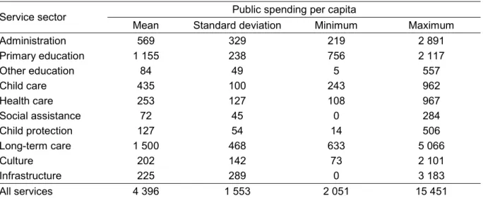
Public services and expenditure. Local government accounts in Norway provide detailed

information on specific expenditure. Table 3.2 summarizes the differences in sector-specific per capita public spending across the 431 municipalities in Norway in 2007. We see that the largest expenditure component is care for the elderly and disabled (long-term care), closely followed by primary education. These two sectors account, on average, for more than half of the total expenditure of municipalities. We also note that there are considerable differences in per capita public spending across municipalities in all service sectors.

Table 3.2 Public spending per capita on different services across municipalities

Public spending per capita Service sector

Mean Standard deviation Minimum Maximum

Administration 569 329 219 2 891

Primary education 1 155 238 756 2 117

Other education 84 49 5 557

Child care 435 100 243 962

Health care 253 127 108 967

Social assistance 72 45 0 284

Child protection 127 54 14 506

Long-term care 1 500 468 633 5 066

Culture 202 142 73 2 101

Infrastructure 225 289 0 3 183

All services 4 396 1 553 2 051 15 451

Note: Numbers are calculated by averaging spending per capita across municipalities for each sector. All numbers are in Euros (exchange rate of 9 NOK per Euro is used).

Table 3.4 shows our classification of local public services into ten different sectors, and the associated target groups. From the administrative registers, we can compute the population shares of different target groups in every municipality. We therefore have a one-to-one correspondence between our population of study and the population shares used in the estimation of the model of local government spending.

The specification of target groups aims at producing mutually exclusive groups within each service sector. By not including partially overlapping target groups, we are able to avoid misleading double-counting of minimum quantities, while at the same time accounting properly for interaction effects pertaining to population subgroups that share more than one of the characteristics that are used by local governments to target the public services.

Cash and extended income. Table 3.3 defines our cash income and extended income measure.

15

income, and public cash transfers, from which direct taxes are subtracted. We use the term extended incometo denote the sum of cash income and the value of in-kind benefits provided through public services. The data on cash income is based on Tax Assessment Files, which are collected from tax records and other administrative registers, rather than interviews and self-reporting methods. The coverage and reliability of Norwegian data on cash income are considered to be very high, as is documented by the fact that the quality of such national datasets of income received the highest rating in a data quality survey in the Luxembourg Income Study database (Atkinson et al., 1995).

Table 3.3 Definition of cash income and extended income

Market income = Employment income (earnings, self-employment income) + Capital income (interest, stock dividends, sale of stocks) Total income = Market income

+ Public cash transfers (e.g. old-age pension, unemployment and disability benefits, child benefits and single parents benefits, social assistance)

Cash income = Total income – direct taxes Extended income = Cash income + non-cash income

3.2 Estimation results

The estimation of the model defined by (2.5)–(2.7) is based on detailed local government accounts and community characteristics for Norwegian municipalities in 2007. The model accounts for spending on the ten service sectors displayed in Table 3.4, and in the estimation we also include the budget surplus (net operating result) as a sector in the model. The budget surplus is treated as a residual sector, which means that the model is representing an extended linear expenditure system, see Lluch (1973). Expenditures are defined exclusive of user fees and employer payroll taxes, and are measured on a per capita basis in the model specification. We estimate the model simultaneously by the method of maximum likelihood.

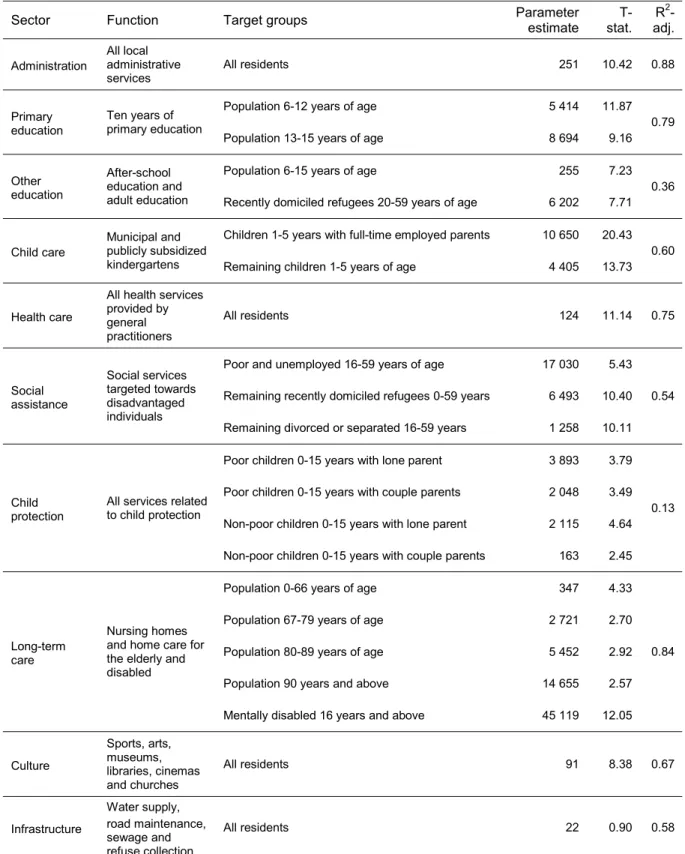
The minimum quantity parameters are displayed in Table 3.4, the unit cost parameters are displayed in Table 3.5, and Table A.1 in Appendix A presents estimates of the marginal budget share parameters. Importantly, the parameter estimates are statistically significant and of the expected signs.

Minimum quantity parameters. Consider the parameter estimates reported in Table 3.4,

16

One main finding is that there is substantial variation in the minimum quantity estimates across target groups. Below we discuss the identified target groups and associated minimum quantities in each of the ten service sectors.

Table 3.4 Estimates of minimum quantity parameters

Sector Function Target groups Parameter _{estimate stat.} T- _adj. R2

-Administration

All local administrative services

All residents 251 10.42 0.88

Primary education

Ten years of primary education

Population 6-12 years of age Population 13-15 years of age

5 414 8 694 11.87 9.16 0.79 Other education After-school education and adult education

Population 6-15 years of age

Recently domiciled refugees 20-59 years of age

255 6 202 7.23 7.71 0.36 Child care Municipal and publicly subsidized kindergartens

Children 1-5 years with full-time employed parents Remaining children 1-5 years of age

10 650 4 405 20.43 13.73 0.60 Health care

All health services provided by general practitioners

All residents 124 11.14 0.75

Social assistance Social services targeted towards disadvantaged individuals

Poor and unemployed 16-59 years of age Remaining recently domiciled refugees 0-59 years Remaining divorced or separated 16-59 years

17 030 6 493 1 258 5.43 10.40 10.11 0.54 Child protection

All services related to child protection

Poor children 0-15 years with lone parent Poor children 0-15 years with couple parents Non-poor children 0-15 years with lone parent Non-poor children 0-15 years with couple parents

3 893 2 048 2 115 163 3.79 3.49 4.64 2.45 0.13 Long-term care Nursing homes and home care for the elderly and disabled

Population 0-66 years of age Population 67-79 years of age Population 80-89 years of age Population 90 years and above Mentally disabled 16 years and above

347 2 721 5 452 14 655 45 119 4.33 2.70 2.92 2.57 12.05 0.84 Culture Sports, arts, museums, libraries, cinemas and churches

All residents 91 8.38 0.67

Infrastructure

Water supply, road maintenance, sewage and refuse collection

All residents 22 0.90 0.58

17

Consider first primary schools, which are compulsory for children 6–15 years of age. It follows that service provision increases as a function of the number of children in this age group. We also see that children aged 6–12 years receive not as much services as children aged 13–15 years. This difference is due to the fact that the latter group faces more extensive and demanding lessons, which requires teachers with higher qualifications.

Local governments operate a few other education services that are not included in the sector for primary education. The service sector “Other education” includes day care facilities for schoolchildren, music schools, special schools and adult education. Except for adult education, the relevant group that benefits from “Other education” is the age group 6-15 years. Adult education is particularly directed toward recently domiciled refugees in the age group 20-59 years. Recently domiciled refugees include refugees who have resided in Norway less than five years.

Moving on to the child-care sector, we see that the service provision increases in the population share of children in pre-school age (1-5 years). The target group is divided into children with and without time employed parents. The marginal cost is higher for the group with full-time employed parents, since these families depend more on professional day-care services, which contributes to higher demand for and coverage in kindergartens.

Next, consider child protection sector, which includes investigation of alleged child abuse, orphan homes, foster care, adoption services, and services aimed at supporting at-risk families so they can remain intact. Children less than 16 years of age are the primary target group for child protection. The estimation results show that the risk and spending is highest among children that belong to a poor family with a lone parent. Risk and spending levels are intermediate for children that are poor with couple parents or non-poor with a lone parent. The lowest spending levels are found among children that are non-poor with couple parents. Poor families include those with incomes below half of median income, where incomes are defined by after-tax private incomes exclusive of social assistance cash transfers. In-kind benefits are not included in the income definition when defining poor families that are highly prone to receive some of the municipal services.

A large share of spending in the social assistance sector is cash transfers to support families with insufficient means from other sources of income. The sector also includes some in-kind

18

benefits that aim to prevent alcohol and drugs abuse and other social problems. The potential recipients are either poor, unemployed, refugees or divorced/separated, or possess different combinations of those characteristics. To account for interaction effects between different characteristics, the potential recipients are divided into mutually exclusive target groups that include all possible combinations of the above mentioned characteristics. The estimates for each subgroup are used to identify target groups with high, intermediate and low risk and spending. The resulting target group classification shows that the poor who are also unemployed is a high-risk group for receiving social assistance. The second target group that receives intermediate spending per person is recently domiciled refugees. The third target group that receives a lower, although significant spending level, is the divorced and separated. Long-term care includes nursing homes, ambulant nurses and home care. The potential recipients are the elderly and disabled. Since elderly people have a higher probability of becoming recipients of long-term care, spending needs are higher for the elderly than for younger people. Subsistence output is increasing with age, and is highest for the elderly 90 years and above. By contrast, spending needs per person is much lower in the age group 0-66 years. However, the group of mentally disabled, which by and large is a subgroup of the age group 0-66 years, is included to account for the additional cost from being mentally disabled. This additional minimum expenditure is rather high, and is above 45,000 Euros per person in the mentally disabled group.

When it comes to administration, municipal health care, culture, and infrastructure, the target group is taken to be the whole population. The financing of local public health services is shared with the central government such that local governments pay for a basic capacity, whilst additional costs due to utilization and health care needs are financed through the national social security system. Thus the local government minimum quantity for health care does not vary as a function of socio-demographic variables. Similarly, for culture, administration and infrastructure, we have not identified any characteristic that yields variation in minimum quantities. Thus, the estimated minimum quantity is a constant, which means that the entire population is treated as the relevant target group.

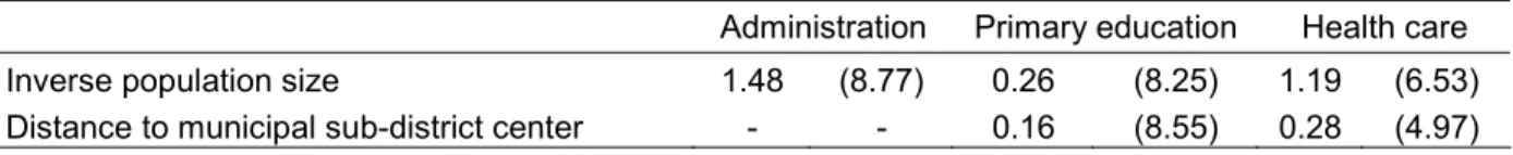
Unit cost parameters. Consider the estimated parameters for variables that affect unit costs, displayed in Table 3.5. These parameters form the basis for the price-adjusted equivalence

19

scales in equation (2.16) and the construction of price indices in equation (2.6). We see that there is significant variation in unit costs in three of the service sectors: administration, primary education and health care.

Table 3.5 Estimates of unit cost parameters

Administration Primary education Health care

Inverse population size 1.48 (8.77) 0.26 (8.25) 1.19 (6.53)

Distance to municipal sub-district center - - 0.16 (8.55) 0.28 (4.97)

Note: T-statistics are in parentheses. Number of observations = 378.

The estimated unit costs in these three service sectors are decreasing as a function of population size. The chosen functional form is the inverse population size, which captures that the decreasing function is convex and close to zero when population is sufficiently large. The positive impact of inverse population size on unit costs may originate from fixed costs in the operation of local governments. Significant parameter estimates for inverse population size are taken as proof of economies of scale. An important reason for smaller municipalities to have higher unit costs is that they use a larger share of resources on administration. Furthermore, class sizes are in general smaller in smaller municipalities, implying more teachers per student and therefore higher costs. Similarly, to maintain a basic capacity of primary physicians in smaller municipalities the physician-patient ratio becomes relatively large, which increases the unit cost.

We also find that greater dispersion of the local settlement pattern increases unit costs in education and health care. The estimated positive relationships are interpreted as reflecting costs of providing services on a decentralized level. For example, when it comes to primary education, municipalities with a high dispersion of settlement tend to supply a decentralized school structure with relatively few students per school and rather small class sizes. The aim is to provide a school structure that does not impose unreasonable travelling distances on the school children. Similarly, patients in primary health care are also entitled to have a physician within reasonable travelling distance. The costs to maintain such services are therefore higher in sparsely populated areas. To capture dispersion of settlement in the municipality, we use an explanatory variable defined as the average distance to the centre of the municipal sub-district. Note that the distance variable has no significant effect in the administration sector.

20

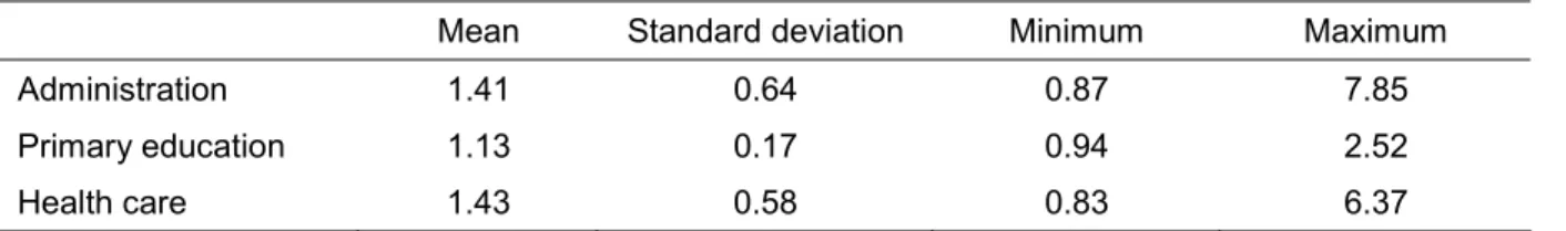
The price indices defined in equation (2.6) reflect the relative differences across municipalities in unit costs for providing different services. Summary statistics for the estimated price indices are reported in Table 3.6. Note that the mean values are above 1 because municipalities with different population sizes are given equal weights, which means that weights per capita are higher in smaller municipalities. Small municipalities are found to encounter high unit costs due to economies of scale and dispersed settlement. Moreover, we find large variation across municipalities in unit costs, particularly in administration and health care.

Table 3.6 Variation in unit costs across municipalities

Mean Standard deviation Minimum Maximum

Administration 1.41 0.64 0.87 7.85

Primary education 1.13 0.17 0.94 2.52

Health care 1.43 0.58 0.83 6.37

Note: Number of observations = 431.

3.3 Allocating local public services

In line with the allocation rule in equation (2.9), we use the above estimates to allocate the values of local public services to individuals. We assume that people who live in the same municipality and belong to the same target group, receive equal non-cash income. Specifically, the in-kind transfer from sector i received by each member of group j is then given by the estimate of u_ij, which may vary across municipalities. Thus, variation in allocated in-kind benefits across people is partly due to differences in individual characteristics that trigger expenditure needs. In addition, there is variation in local government spending across service sectors, as well as in spending priorities on different target groups.

The target groups that are treated as recipients in the analysis may deviate from the group of actual recipients. There are two reasons for this. First, we usually do not observe the group of actual recipients. Hence, the identified target groups serve to approximate groups of actual recipients. Although the simulated recipients are not necessarily the same as the actual recipients, a good approximation of the underlying distributional profiles of public services should be obtained, provided that the relevant characteristics of recipients are taken into

21

account.6 _{Second, in line with Smeeding et al. (1993), the services child protection, social}

assistance, health care, and long-term care are viewed as insurance benefits received by everyone covered by the insurance scheme, regardless of actual use. The received expenditure of such services is interpreted as expected non-cash income, which depends on the risk of becoming a recipient. Risk factors are accounted for by the characteristics of target groups that are assumed to receive the different services.

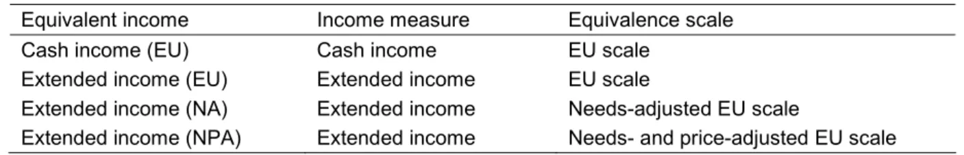
3.4 Equivalent income definitions

When analyzing poverty and inequality among households of varying size and composition, it is necessary to adjust the measure of income to enable comparison across individuals. As discussed above, interpersonal comparison of income is typically achieved by using equivalence scales. We consider four different definitions of equivalent income, depending on whether we consider cash or extended income and how we adjust for differences in needs for non-cash income. The different definitions of equivalent income are displayed in Table 3.6. Table 3.6 Alternative definitions of equivalent income

Equivalent income Income measure Equivalence scale

Cash income (EU) Cash income EU scale

Extended income (EU) Extended income EU scale

Extended income (NA) Extended income Needs-adjusted EU scale

Extended income (NPA) Extended income Needs- and price-adjusted EU scale

Following the previous literature in inequality and poverty closely, we use the EU scale to adjust for differences in cash income needs. This yields the measure of equivalent cash income, which typically forms the basis for studies of poverty and inequality. To obtain the measure of extended income, we add the value of non-cash income to cash income. In line with previous studies, we use the same scale to adjust for needs for extended income as is used to adjust cash income. Consequently, extended income is adjusted by the EU scale. Thus, the first step is to change the income measure without changing the equivalence scale. The second step is to change the equivalence scale for extended income by taking into account the needs for public services of different target groups. Needs-adjusted extended equivalent income is derived by using the NA scale from Section 2.3 to adjust for differences in needs. The NA scale is a weighted average of the EU scale for cash income and the NC scale for non-cash income. The

6 _{In the child care sector we also utilize additional information about coverage in kindergartens on the municipal level.}

22

NA scale assumes that the sector-specific price indices are constant across municipalities, which is a special case of the NPA scale defined in equation (2.19). Thus, the third step is to introduce price adjustment in the equivalence scale, so the needs adjustment is based on the NPA scale, which yields needs- and price-adjusted extended equivalent income.

In order to empirically implement the NA and NPA scales, it is necessary to assign a value to the weight they give to cash income, _rdefined in equation (2.19). In particular, we assume that the minimum quantity of cash income for the reference group,_0r, is equal to the minimum pension entitlement for a single person in the social security system. The estimate of _r is equal to 0.95. As a robustness check, we have set _0r equal to the poverty threshold derived from the equivalent cash income in the entire population. As our results barely move, we only report the results where the minimum pension is used to determine _r.

3.5 Measuring inequality and poverty

Inequality measures. To summarize the informational content of the Lorenz curve and to

achieve rankings of intersecting Lorenz curves, the conventional approach is to employ the Gini-coefficient. To examine the extent to which the empirical results depend on the choice of inequality measure, the Gini-coefficient is typically complemented with measures from the Atkinson or Theil family. However, the Gini-coefficient and inequality measures from the Atkinson or the Theil family have distinct theoretical foundations which make it inherently difficult to evaluate their capacities as complimentary measures of inequality. As demonstrated by Aaberge (2007), an alternative approach for examining inequality in the distribution of income is to rely on Gini’s Nuclear Family defined by

(3.1) 1 2





0

( ) k ( ) , 1,2,3 k

C F k u



 u L u du k

where C1 is equivalent to a measure of inequality that was proposed by Bonferroni (1930), whilst C2 is the Gini coefficient. As demonstrated by Aaberge (2000, 2007) C1 exhibits strong

downside inequality aversion and is particularly sensitive to changes that concern the poor part of the population, whilst C2 normally pays more attention to changes that take place in the

middle part of the income distribution. The C3-coefficient exhibits upside inequality aversion

23

and is thus particularly sensitive to changes that occur in the upper part of the income distribution. In this paper, we will examine the sensitivity of the empirical results to the choice of inequality measure by complementing the information provided by C2 with its two close

relatives C1 and C3. Hence, we meet the most common criticism of the Gini-coefficient, namely

that it is insensitive to redistribution of income at the lower end of the distribution.

Poverty thresholds. We follow common practice in most developed countries and specify a set of poverty thresholds as a certain fraction of the median income. Specifically, we will focus on a set of poverty thresholds defined as 60 per cent of the median of the chosen measure of income. Recognizing the inherent arbitrariness of specifying an exact poverty threshold, it can be instructive to apply other thresholds to evaluate the robustness of the results. Moreover, by applying multiple thresholds one can obtain a fuller picture of the problem of poverty in a society. Thus we will supplement the analysis with poverty thresholds defined as 50 percent of the median of the chosen measure of income.7

4. Distributional impact of public services

This section examines the impact on inequality and poverty estimates of accounting for non-cash income from local public services, and, moreover, adjusting for differences in needs for such services across individuals.

4.1 Main results

Overall inequality and poverty. Table 4.1 reports the income shares by decile for each measure of equivalent income outlined in Table 3.6. As the distribution of income may vary substantially within each decile group, we need to be cautious in drawing firm conclusions from Table 4.1 about the distributional impact of public services. With this caveat in mind, the second column indicates that local public spending is quite redistributive, given the cash income shares reported in the first column. We find that the income shares increase in lower decile groups and decrease in higher decile groups when non-cash income is added to cash income. However, the third column suggests that substituting the EU-scale with the NA-scale in the needs-adjustment of extended income offsets some of the redistributional impact of

7 _{Following official poverty statistics in Norway and several other developed countries, students and wealthy individuals are}

not counted as poor. Because we lack credible data on wealth, an individual is classified as wealthy if he or she is registered with equivalent gross financial capital greater than three times the median equivalent cash income.

24

public services. The final column shows that price-adjustment appear to have little impact on how needs-adjusted extended equivalent income is distributed across the decile groups.

Table 4.1 Income shares by deciles for different income measures

Income share by decile (%)

Cash income Extended income

Decile

EU EU NA NPA

1st 3.7 4.4 4.1 4.1

2nd 6.0 6.7 6.3 6.3

3rd 7.1 7.7 7.2 7.2

4th 8.0 8.5 8.0 8.0

5th _{8.8 9.2 8.8 8.8}

6th 9.6 9.8 9.6 9.6

7th 10.5 10.5 10.5 10.5

8th _{11.6 11.4 11.6 11.6}

9th 13.3 12.7 13.3 13.3

10th 21.2 19.2 20.5 20.6

Overall mean 32 317 38 308 31 136 31 146

Note: NA: Needs-adjusted EU scale. NPA: Needs-and price-adjusted EU scale. Income is reported in Euros (exchange rate of 9 NOK per Euro is used).

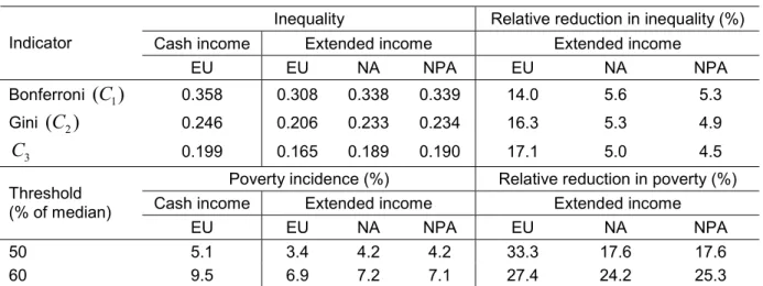
Table 4.2 Inequality and poverty by income measure

Inequality Relative reduction in inequality (%)

Cash income Extended income Extended income

Indicator

EU EU NA NPA EU NA NPA

Bonferroni (C₁) 0.358 0.308 0.338 0.339 14.0 5.6 5.3

Gini (C₂) 0.246 0.206 0.233 0.234 16.3 5.3 4.9

3

C 0.199 0.165 0.189 0.190 17.1 5.0 4.5

Poverty incidence (%) Relative reduction in poverty (%)

Cash income Extended income Extended income

Threshold (% of median)

EU EU NA NPA EU NA NPA

50 5.1 3.4 4.2 4.2 33.3 17.6 17.6

60 9.5 6.9 7.2 7.1 27.4 24.2 25.3

Note: NA: Needs-adjusted EU scale. NPA: Needs-and price-adjusted EU scale. The three inequality measures are calculated for each of the four equivalent income distributions. Poverty thresholds are calculated on the basis of median in each of the four income distributions. For each income measure, the relative reduction in inequality/poverty is given as the per cent decrease compared to inequality/poverty when cash income is used.

To investigate further the distributional impact of public services, the upper panel of Table 4.2 employs the inequality measures outlined above. When comparing the first and the second column, we see that including non-cash income reduces inequality by about 15 percent. This suggests that public services are targeted toward individuals with relatively low cash income. However, as is clear from the third column, using our method to adjust for differences in needs offset about two-third of the inequality reduction stemming from the inclusion of non-cash

25

income. Hence, the method used to make needs adjustment appears to be fairly important when drawing lessons about the redistributive nature of public services. Finally, column five demonstrates that allowing for variation across municipalities in unit costs for producing public services has little impact on inequality.

When comparing rows 1-3, we see that the findings are fairly robust to the choice of inequality measure. Interestingly, the inequality measure that is most sensitive to changes in the lower part of the distribution, C1, records the smallest (percentage) reduction when applying the EU scale

to extended income. However, the picture is reversed when using the NA or the NPA scale, in which case C1 records the largest (percentage) decrease in inequality. This illustrates that

redistribution of extended income at the lower end of the distribution plays a more important role when using our method to adjust for differences in needs.

The lower panel of Table 4.2 shows the share of the population with income below the poverty line according to the different definitions of income. We see that poverty rates are reduced by almost one-third, when we consider extended income instead of the conventional cash income measure. However, using our method to adjust for differences in needs offsets some of the poverty reduction, in particular when the relatively low poverty threshold of 50 percent of the median is used. This indicates that there is a concentration of individuals with low cash income who have relatively high needs for public services, which is ignored when one uses the EU scale to adjust extended income. Just as for the inequality estimates, allowing for variation across municipalities in unit costs for producing public services has little impact on poverty incidence.

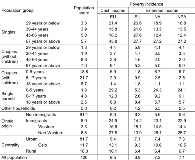
Poverty profile. Below,we investigate the impact of public services on the poverty profile. For brevity, we only report results using a poverty threshold of 60 percent of the median.

Table 4.3 shows the effect of accounting for local public services on poverty rates by household type. When focusing on cash income, the poverty rates are rather high among elderly (mostly female) living in single person households, due to the fact that the poverty thresholds exceed the guaranteed minimum pension. However, as elderly people receive a high level of publicly provided care and health services, their poverty rates drop radically when we focus on extended income. The same is true for households with children, especially single parents, since they are

26

major recipients of services such as education and child care. For these subgroups, however, the poverty rates rise again when we use our method to adjust for differences in needs. Due to the age structure and the relatively high fertility rate of Non-Western immigrants, their poverty rates also decline considerably when non-cash income are taken into account. The relatively high levels of non-cash income also reflect higher needs for public services, as their poverty rates rise again when we make needs adjustment according to the NA scale. The groups that receive the least non-cash income are singles and couples without children in the pre-retirement phase. The poverty rates for these households therefore increase when we consider extended income. However, their poverty rates fall when we use our method to adjust for needs. This finding comes as no surprise, as these households have no children who need child care or education, and their need for publicly provided long-term care is small.

Table 4.3 Poverty profile in different population groups by income measure

Poverty incidence

Cash income Extended income

Population group Population _share

EU EU NA NPA

29 years or below 3.3 21.4 26.6 18.9 18.8

30-44 years 3.9 15.8 21.6 13.5 13.5

45-66 years 5.0 18.2 27.6 12.4 12.4

Singles

67 years or above 5.7 45.8 27.7 27.2 27.2

29 years or below 1.3 4.4 5.9 4.1 4.1

30-44 years 1.9 3.7 4.7 3.5 3.5

45-66 years 8.6 2.8 4.6 2.0 2.0

Couples (without children)

67 years or above 7.0 9.1 5.3 5.0 5.0

0-5 years 18.8 6.9 1.8 6.7 6.7

6-17 years 21.7 2.9 0.9 2.5 2.5

Couples (with

children) _{18 years or above 8.7 1.4 1.8 1.1 1.1}

0-5 years 1.8 29.2 5.3 24.3 24.1

6-17 years 4.8 12.3 2.6 9.2 9.1

Single parents

18 years or above 2.5 6.8 8.4 5.7 5.7

Other households 5.0 6.2 4.2 5.5 5.5

Non-immigrants 91.1 8.0 6.2 5.6 5.6

Immigrants 8.9 24.9 14.2 23.1 22.9

Western 2.3 16.6 15.1 14.5 14,4

Ethnic origin

Non-Western 6.6 27.8 13.9 26.1 25,7

Urban 81.7 9.4 7.1 7.4 7.3

Oslo 11.7 13.1 9.3 10.6 10.5

Centrality

Rural 18.3 10.1 6.4 6.4 6.7

All population 100 9.5 6.9 7.2 7.1

Note: NA: Needs-adjusted EU scale. NPA: Needs-and price-adjusted EU scale. Poverty thresholds are calculated as 60 percent of the median in each of the four income distributions.

27

Table 4.3 also shows poverty incidence by centrality. The results show that incorporating public services into the income measure reduces the poverty rates in rural areas relative to urban areas and, especially, compared to Oslo. When we use our method to adjust for differences in needs, a similar pattern appears: While the poverty rate in rural areas is unchanged, we see that poverty rates rise again in urban areas (especially Oslo). This indicates that public transfers targeted towards individuals living in urban areas often reflect higher needs.

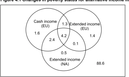
Figure 4.1 Changes in poverty status for alternative income measures

Note: NA: Needs-adjusted EU scale. Poverty thresholds are calculated as 60 percent of the median in each of the three income distributions.

Figure 4.1 demonstrates the degree of overlap in individuals’ poverty status when changing the measure of equivalent income. We immediately see that accounting for the value of non-cash income and the method used to adjust for differences in needs not only change the poverty rate, but also which individuals that are classified as poor. Specifically, only 4.2 percentage points are poor according to all three income measures. The overlap in poverty status is largest between cash income and the extended income measure using our method for needs adjustment.

4.2 Sensitivity analysis

Balanced budget. In the analysis above, we have followed standard practice in empirical

analysis of the distributional impact of public services in disregarding that the cost of their provision may differ from the direct taxes levied on individuals and households.8 In principle, if we include the value of public services we should also take into account the associated cost borne by the individuals. A possible concern is, therefore, that the direct taxes and the public

8 _{A notable exception is Garfinkel et al. (2006), who try to balance the expenditure on public services and the tax revenues.} Cash income

(EU) Extended income

(EU)

Extended income (NA) 4.2

1.3

2.4

0.1

1.4 1.6

0.5