Approximate Bayesian computation in large-scale structure: constraining the galaxy-halo connection

Approximate Bayesian computation in large-scale structure: constraining

the galaxy–halo connection

ChangHoon Hahn,

†

Mohammadjavad Vakili,

†

Kilian Walsh,

Andrew P. Hearin,

David W. Hogg

and Duncan Campbell

1_{Center for Cosmology and Particle Physics, Department of Physics, New York University, 726 Broadway, New York, NY 10003, USA} 2_{Yale Center for Astronomy and Astrophysics, Yale University, New Haven, CT 06520, USA}

3_{Flatiron institute, 160 Fifth Avenue, New York, NY 10010, USA}

4_{Center for Data Science, New York University, 60 Fifth Ave, New York, NY 10011, USA} 5_{Max-Planck-Institut f¨ur Astronomie, K¨onigstuhl 17, D-69117 Heidelberg, Germany} 6_{Department of Astronomy, Yale University, New Haven, CT 06511, USA}

Accepted 2017 April 10. Received 2017 March 14; in original form 2016 July 5

A B S T R A C T

Standard approaches to Bayesian parameter inference in large-scale structure assume a Gaus-sian functional form (chi-squared form) for the likelihood. This assumption, in detail, cannot be correct. Likelihood free inferences such as approximate Bayesian computation (ABC) re-lax these restrictions and make inference possible without making any assumptions on the likelihood. Instead ABC relies on a forward generative model of the data and a metric for measuring the distance between the model and data. In this work, we demonstrate that ABC is feasible for LSS parameter inference by using it to constrain parameters of the halo occupa-tion distribuoccupa-tion (HOD) model for populating dark matter haloes with galaxies. Using specific implementation of ABC supplemented with population Monte Carlo importance sampling, a generative forward model using HOD and a distance metric based on galaxy number den-sity, two-point correlation function and galaxy group multiplicity function, we constrain the HOD parameters of mock observation generated from selected ‘true’ HOD parameters. The parameter constraints we obtain from ABC are consistent with the ‘true’ HOD parameters, demonstrating that ABC can be reliably used for parameter inference in LSS. Furthermore, we compare our ABC constraints to constraints we obtain using a pseudo-likelihood function of Gaussian form with MCMC and find consistent HOD parameter constraints. Ultimately, our results suggest that ABC can and should be applied in parameter inference for LSS analyses.

Key words: methods: data analysis – methods: statistical – galaxies: haloes – dark matter – large-scale structure of Universe.

1 I N T R O D U C T I O N

Cosmology was revolutionized in the 1990s with the introduction of likelihoods – probabilities for the data given the theoretical model – for combining data from different surveys and perform-ing principled inferences of the cosmological parameters (White &

Scott1996; Riess et al.1998). Nowhere has this been more true than

in cosmic microwave background (CMB) studies, where it is nearly possible to analytically evaluate a likelihood function that involves

no (or minimal) approximations (Oh, Spergel & Hinshaw1999;

Eriksen et al.2004; Wandelt, Larson & Lakshminarayanan2004;

Planck Collaboration XVI2014; Planck Collaboration XIII2016).

_{E-mail:[email protected](CHH);[email protected](MV)} †These authors have contributed equally to the paper.

Fundamentally, the tractability of likelihood functions in cosmol-ogy flows from the fact that the initial conditions are exceedingly

close to Gaussian in form (Planck Collaboration XVII2016; Planck

Collaboration XX2016) and that many sources of measurement

noise are also Gaussian (Knox1995; Leach et al.2008).

Likeli-hood functions are easier to write down and evaluate when things are closer to Gaussian, so at large scales and in the early universe. Hence, likelihood analyses are ideally suitable for CMB data.

In large-scale structure (LSS) with galaxies, quasars and quasar absorption systems as tracers, formed through non-linear

grav-itational evolution and biasing, the likelihood cannot be

Gaus-sian. Even if the initial conditions are perfectly Gaussian, the growth of structure creates non-linearities that are non-Gaussian

(see Bernardeau et al.2002for a comprehensive review).

Galax-ies form within the density field in some complex manner that is

modelled only effectively (Dressler1980; Kaiser1984; Santiago &

2017 The Authors

Strauss1992; Steidel et al.1998; see Somerville & Dav´e2015for a recent review). Even if the galaxies were a Poisson sampling of

the density field, which they are not (Mo & White1996; Somerville

et al.2001; Casas-Miranda et al.2002), it would be tremendously

difficult to write down even an approximate likelihood function

(Ata, Kitaura & M¨uller2015).

The standard approach makes the strong assumption that the likelihood function for the data can be approximated by a pseudo-likelihood function that is a Gaussian probability density in the space of the two-point correlation function estimate. It is also typically limited to (density and) two-point correlation function (2PCF) mea-surements, assuming that these measurements constitute sufficient statistics for the cosmological parameters. As Hogg (in prepara-tion) demonstrates, the assumption of a Gaussian pseudo-likelihood function cannot be correct (in detail) at any scale, since a correla-tion funccorrela-tion, being related to the variance of a continuous field, must satisfy non-trivial positive-definiteness requirements. These requirements truncate function space such that the likelihood in that function space could never be Gaussian. The failure of this assumption becomes more relevant as the correlation function be-comes better measured, so it is particularly critical on intermediate scales, where neither shot noise nor cosmic variance significantly influence the measurement.

Fortunately, these assumptions are not required for cosmological inferences, because high-precision cosmological simulations can be used to directly calculate LSS observables. Therefore, we can sim-ulate not just the one- or two-point statistics of the galaxies but also any higher order statistics that might provide additional constrain-ing power on a model. In principle, there is therefore no strict need to rely on these common but specious analysis assumptions as it is possible to calculate a likelihood function directly from simulation outputs.

Of course, any naive approach to sufficiently simulating the data would be ruinously expensive. Fortunately, there are principled, (relatively) efficient methods for minimizing computation and de-livering correct posterior inferences, using only a data simulator and some choices about statistics. In this work, we use approximate

Bayesian computation – ABC – which provides arejection sampling

framework (Pritchard et al.1999) that relaxes the assumptions of

the traditional approach.

ABC approximates the posterior probability distribution func-tion (model given the data) by drawing proposals from the prior over the model parameters, simulating the data from the pro-posals using a forward generative model, and then rejecting the proposals that are beyond a certain threshold ‘distance’ from the data, based on summary statistics of the data. In practice, ABC is used in conjunction with a more efficient sampling operation like

Population Monte Carlo (PMC; Del Moral, Doucet & Jasra2006).

PMC initially rejects the proposals from the prior with a relatively large ‘distance’ threshold. In subsequent steps, the threshold is up-dated adaptively, and samples from the proposals that have passed the previous iteration are subjected to the new, more stringent,

threshold criterion (Beaumont et al. 2009). In principle, the

dis-tance metric can be any positive definite function that compares various summary statistics between the data and the simulation.

In the context of astronomy, this approach has been used in a wide range of topics including image simulation calibration for wide field

surveys (Akeret et al.2015), the study of the morphological

prop-erties of galaxies at high redshifts (Cameron & Pettitt2012), stellar

initial mass function modelling (Cisewski et al., in preparation) and cosmological inference with with weak-lensing peak counts (Lin &

Kilbinger2015; Lin, Kilbinger & Pires2016), Type Ia Supernovae

(Weyant, Schafer & Wood-Vasey2013) and galaxy cluster number

counts (Ishida et al.2015).

In order to demonstrate that ABC can be tractably applied to pa-rameter estimation in contemporary LSS analyses, we narrow our focus to inferring the parameters of a halo occupation distribution (HOD) model. The foundation of HOD predictions is the halo model of LSS, that is, collapsed dark matter haloes are biased tracers of

the underlying cosmic density field (Press & Schechter1974; Bond

et al.1991; Cooray & Sheth2002). The HOD specifies how the dark

matter haloes are populated with galaxies by modelling the

proba-bility that a given halo hostsNgalaxies subject to some

observa-tional selection criteria (Lemson & Kauffmann1999; Seljak2000;

Scoccimarro et al. 2001; Berlind & Weinberg 2002; Zheng

et al. 2005). This statistical prescription for connecting galaxies

to haloes has been remarkably successful in reproducing the galaxy clustering, galaxy–galaxy lensing and other observational

statis-tics (Miyatake et al. 2015; Rodr´ıguez-Torres et al. 2016), and

is a useful framework for constraining cosmological parameters

(van den Bosch, Mo & Yang2003; Tinker et al.2005; Cacciato

et al.2013; More et al.2013) as well as galaxy evolution models

(Conroy & Wechsler2009; Tinker, Wetzel & Conroy2011;

Leau-thaud et al.2012; Behroozi, Wechsler & Conroy2013b; Tinker

et al.2013; Walsh & Tinker, in preparation).

More specifically, we limit our scope to a likelihood analysis of HOD model parameter space, keeping cosmology fixed. We for-ward model galaxy survey data by populating pre-built dark matter

halo catalogues obtained from high-resolutionN-body simulations

(Klypin, Trujillo-Gomez & Primack2011; Riebe et al.2013)

us-ingHALOTOOLS1(Hearin et al.2016a), an open-source package for modelling the galaxy–halo connection. Equipped with the forward model, we use summary statistics such as number density, two-point correlation function, galaxy group multiplicity function (GMF) to infer HOD parameters using ABC.

In Section 2, we discuss the algorithm of the ABC-PMC pre-scription we use in our analyses. This includes the sampling method itself, the HOD forward model and the computation of summary statistics. Then in Section 3.1, we discuss the mock galaxy cat-alogue, which we treat as observation. With the specific choices of ABC-PMC ingredients, which we describe in Section 3.2, in Section 3.3, we present the results of our parameter inference us-ing two sets of summary statistics, number density and 2PCF and number density and GMF. We also include in our results, analogous parameter constraints from the standard MCMC approach, which we compare to ABC results in detail, Section 3.4. Finally, we discuss and conclude in Section 4.

2 M E T H O D S

2.1 Approximate Bayesian computation

ABC is based on rejection sampling, so we begin this section with a brief overview of rejection sampling. Broadly speaking, rejection sampling is a Monte Carlo method used to draw samples from a

probability distribution,f(α), which is difficult to directly sample.

The strategy is to draw samples from an instrumental distribution

g(α) that satisfies the conditionf(α)<Mg(α) for allα, whereM>1

is some scalar multiplier. The purpose of the instrumental

distribu-tiong(α) is that it is easier to sample thanf(α) (see Bishop2007

and references therein).

1_{http://halotools.readthedocs.org}

In the context of simulation-based inference, the ultimate goal is

to sample from the joint probability of a simulationXand parameters

θgiven observed dataD, the posterior probability distribution. From

Bayesian rule, this posterior distribution can be written as

p(θ, X|D)= p(D|X)p(X|θ)π(θ)

Z , (1)

whereπ(θ) is the prior distribution over the parameters of interest

andZis the evidence,

Z=

dθdX p(D|X)p(X|θ)π(θ), (2)

where the domain of the integral is all possible values ofXand

θ. Sincep(θ, X|D) cannot be directly sampled, we use rejection

sampling with instrumental distribution

q(θ, X)=p(X|θ)π(θ) (3)

and the choice of

M= maxp_Z(D|X) >1. (4)

Note that we do not ever need to knowZ. The choices ofq(θ, X)

andMsatisfy the condition

p(θ, X|D)< Mq(θ, X), (5)

so we can samplep(θ, X|D) by drawing θ, X fromq(θ, X). In

practice, this is done by first drawingθfrom the priorπ(θ) and then

generating a simulationX=f(θ) via the forward model. Thenθ, X

is accepted if

p(θ, X|D) Mq(θ, X) =

p(D|X)

maxp(D|X) > u, (6)

whereuis drawn fromUniform[0,1]. By repeating this rejection

sampling process, we sample the distributionp(θ, X|D) with the

set ofθandXthat are accepted.

At this stage, ABC distinguishes itself by postulating thatp(D|X),

the probability of observing dataDgiven simulationX (not the

likelihood), is proportional to the probability of the distance between the data and the simulation X being less than an arbitrarily small

threshold

p(D|X)∝p(ρ(D, X)< ), (7)

whereρ(D,X) is the distance between the dataDand the simulation

X. Equation (7) along with the rejection sampling acceptance criteria

(equation 6) leads to the acceptance criteria for ABC:θis accepted

ifρ(D,X)< .

The distance function is a positive definite function that measures the closeness of the data and the simulation. The distance can be a vector with multiple components where each component is a distance between a single summary statistic of the data and that of

the simulation. In that case, the thresholdin equation (7) will also

be a vector with the same dimensions.θis accepted if the distance

vector is less than the threshold vector for every component. The ABC procedure begins, in the same fashion as rejection

sam-pling, by drawingθfrom the prior distributionπ(θ). The simulation

is generated fromθusing the forward model,X=f(θ). Then the

distance between the data and simulation,ρ(D, X), is calculated

and compared to. Ifρ(D, X)<,θis accepted. This process is

repeated until we are left with a sample ofθ that all satisfy the

distance criteria. This final ensemble approximates the posterior

probability distributionp(θ, X|D).

As it is stated, the ABC method poses some practical challenges.

If the thresholdis arbitrarily large, the algorithm essentially

sam-ples from the priorπ(θ). Therefore, a sufficiently small threshold

is necessary to sample from the posterior probability distribution. However, an appropriate value for the threshold is not known a priori. Yet, even if an appropriate threshold is selected, a small threshold requires the entire process to be repeated for many draws

of θ from π(θ) until a sufficient sample is acquired. This often

presents computation challenges.

We overcome some of the challenges posed by the above ABC method by using a population Monte Carlo (PMC) algorithm as our sampling technique. PMC is an iterative method that performs

rejec-tion sampling over a sequence ofθdistributions ({_p1(θ), ..., pT(θ)}

forTiterations), with a distance threshold that decreases at each

iteration of the sequence.

Algorithm 1The procedure for ABC-PMC 1: if_t=1 :then

2: fori=1, ..., Ndo

3: //This loop can now be done in parallel for all i

4: whileρ(X, D)> tdo 5: θ_t∗←π(θ)

6: X=f(θt∗) 7: end while 8: θt(i)←θt∗ 9: w(ti)←1/N 10: end for 11: end if

12: ift=2, ..., T :then 13: fori=1, ..., Ndo

14: //This loop can now be done in parallel for all i

15: whileρ(X, D)> tdo

16: Drawθt∗from{θt−1}with probabilities{wt−1}

17: θ_t∗←K(θ_t∗, .) 18: X=f(_θt∗) 19: end while 20: θt(i)←θt∗ 21: w(ti)←π(θ

(i)

t )/

N

j=1

w_t(i−1) K(θt(−1j), θ

(i)

t )

22: end for 23: end if

As illustrated in Algorithm 1, for the first iterationt= 1, we

begin with an arbitrarily large distance threshold 1. We drawθ

(hereafter referred to as particles) from the prior distributionπ(θ).

We forward model the simulationX=f(θ), calculate the distance

ρ(D,X), compare this distance to1, and then accept or reject the

θdraw. Because we set1arbitrarily large, the particles essentially

sample the prior distribution. This process is repeated until we

acceptNparticles. We then assign equal weights to theNparticles:

wi

1=1/N.

For subsequent iterations (t_>1), the distance threshold is set such

thati,t< i,t−1for all componentsi. Although there is no general

prescription, the distance thresholdi,tcan be assigned based on

the empirical distribution of the accepted distances of the previous

iteration,t−1. In Weyant et al. (2013), for instance, the threshold

of the second iteration is set to the 25th percentile of the distances in

the first iterations; afterwards in the subsequent iterations,t,tis set

to the 50th percentile of the distances in the previoust−1 iteration.

Alternatively, Lin & Kilbinger (2015) settto the median of the

distances from the previous iteration. In Section 3, we describe our prescription for the distance threshold, which follows Lin &

Kilbinger (2015).

Oncetis set, we draw a particle from the previous weighted set

of particlesθ_t−1. This particle is perturbed by a kernel, set to the

covariance ofθ_t−1. Then once again, we generate a simulation by

forward modellingX=f(θi), calculate the distanceρ(X,D) and

compare the distance to the new distance threshold (t) in order to

accept or reject the particle. This process is repeated until we

assem-ble a new set ofNparticlesθ_t. We then update the particle weights

according to the kernel, the prior distribution, and the previous set of weights, as described in Algorithm 1. The entire procedure is

then repeated for the next iteration,t+1.

There are a number of ways to specify the perturbation kernel in the ABC-PMC algorithm. A widely used technique is to define the perturbation kernel as a multivariate Gaussian centred on the weighted mean of the particle population with a covariance matrix set to the covariance of the particle population. This perturbation kernel is often called the global multivariate Gaussian kernel. For a thorough discussion of various schemes for specifying the

pertur-bation kernel, we refer the reader to Filippi et al. (2011).

The iterations continue in the ABC-PMC algorithm until conver-gence is confirmed. One way to ensure converconver-gence is to impose a threshold for the acceptance ratio, which is measured in each iter-ation. The acceptance ratio is the ratio of the number of proposals accepted by the distance threshold, to the full number of proposed particles at every step. Once the acceptance ratio for an iteration falls below the imposed threshold, the algorithm has converged and is suspended. Another way to ensure convergence is by monitoring the

fractional change in the distance threshold (t/t−1−1) after each

iteration. When the fractional change becomes smaller than some specified tolerance level, the algorithm has reached convergence. Another convergence criterion is through the derived uncertainties of the inferred parameters measured after each iteration. When the uncertainties stabilize and show negligible variations, convergence is ensured. In Section 3.2, we detail the specific convergence criteria used in our analysis.

2.2 Forward model

2.2.1 Halo occupation modelling

ABC requires a forward generative model. In LSS studies, this implies a model that is able to generate a galaxy catalogue. We then calculate and compare summary statistics of the data and model catalogue in an identical fashion In this section, we describe the forward generative model we use within the framework of the HOD. The assumption that galaxies reside in dark matter haloes is the bedrock underlying all contemporary theoretical predictions for galaxy clustering. The HOD is one of the most widely used ap-proaches to characterizing this galaxy–halo connection. The central

quantity in the HOD isp(Ng|Mh), the probability that a halo of mass

MhhostsNggalaxies.

The most common technical methods for estimating the

theoret-ical galaxy 2PCF utilize the first two moments ofP, which contain

the necessary information to calculate the one- and two-halo terms of the galaxy correlation function:

1+ξgg1h(r)

1

4πr2_n¯2

g

dMh

dn

dMh

gg(r|Mh)×

Ng(Ng−1)|Mh

,

(8)

and

ξgg2h(r)ξmm(r)

1 ¯ ng

dMh

dn

dMh

Ng|Mh

bh(Mh) 2

(9)

In equations (8) and (9), ¯_ngis the galaxy number density, dn/dMh

is the halo mass function, the spatial bias of dark matter haloes is

bh(Mh) andξmmis the correlation function of dark matter. If we

rep-resent the spherically symmetric intra-halo distribution of galaxies

by a unit-normalizedng(r), then the quantity gg(r) appearing in the

above two equations is the convolution ofng(r) with itself. These

fitting functions are calibrated usingN-body simulations.

Fitting function techniques, however, require many simplifying assumptions. For example, equations (8) and (9) assume that the galaxy distribution within a halo is spherically symmetric. These equations also face well-known difficulties of properly treating halo exclusion and scale-dependent bias, which results in additional inac-curacies commonly exceeding the 10 per cent level (van den Bosch

et al.2013). Direct emulation methods have made significant

im-provements in precision and accuracy in recent years (Heitmann

et al.2009,2010); however, a labour- and computation-intensive

interpolation exercise must be carried out each time any alternative statistic is explored, which is one of the goals of this work.

To address these problems, throughout this paper we make no

ap-peal to fitting functions or emulators. Instead, we use theHALOTOOLS

package to populate dark matter haloes with mock galaxies and then calculate our summary statistics directly on the resulting galaxy catalogue with the same estimators that are used on observational

data (Hearin et al.2016a). Additionally, through our forward

mod-elling approaching, we are able to explore observables beyond the 2PCF, such as the group multiplicity function, for which there is no available fitting function. This framework allows us to use group multiplicity function for providing quantitative constraints on the galaxy–halo connection. In the following section, we will show that using this observable, we can obtain constraints on the HOD pa-rameters comparable to those found from the 2PCF measurements. For the fiducial HOD used throughout this paper, we use the

model described in Zheng et al. (2007). The occupation statistics

of central galaxies follow a nearest integer distribution with first moment given by

Ncen = 1 2

1+erf

logM−logMmin

σlogM .

(10)

Satellite occupation is governed by a Poisson distribution with the mean given by

Nsat = Ncen

M−M0 M1

_α

. (11)

We assume that central galaxies are seated at the exact centre of the host dark matter halo and are at rest with respect to the halo velocity,

defined according toRockstarhalo finder (Behroozi, Wechsler &

Wu2013a) as the mean velocity of the inner 10 per cent of particles in the halo. Satellite galaxies are confined to reside within the virial

radius following an NFW spatial profile (Navarro et al.2004) with

a concentration parameter given by thec(M) relation (Dutton &

Macci`o2014). The peculiar velocity of satellites with respect to their

host halo is calculated according to the solution of the Jeans equation

of an NFW profile (More, van den Bosch & Cacciato2009). We

refer the reader to Hearin et al. (2016b), Hearin et al. (2016a) and

http://halotools.readthedocs.iofor further details.

For the halo catalogue of our forward model, we use the publicly

availableRockstar(Behroozi et al.2013a) halo catalogues of the

MultiDarkcosmologicalN-body simulation (Riebe et al.2013).2

2_{In particular, we use thehalotools_alpha_version2version of}

this catalogue, made publicly available as part ofHalotools.

MultiDarkis a collisionless dark-matter onlyN-body simulation.

TheCDM cosmological parameters ofMultiDarkarem=0.27,

=0.73,b=0.042,ns=0.95,σ8=0.82 andh=0.7. The

gravity solver used in theN-body simulation is the Adaptive

Re-finement Tree code (ART; Kravtsov, Klypin & Khokhlov1997) run

on 20483_{particles in a 1h}−1_{Gpc periodic box.MultiDarkparticles}

have a mass ofmp8.72×108h−1M ; the force resolution of

the simulation is7h−1kpc.

One key detail of our forward generative model is that when

we populate theMultiDarkhaloes with galaxies, we do not

pop-ulate the entire simulation volume. Rather, we divide the volume into a grid of 125 cubic subvolumes, each with side lengths of

200h−1_{Mpc. We refer to these subvolumes as{BOX1}

, ...,BOX125}. The first subvolume is reserved to generate the mock observations that we describe in Section 3.1. When we simulate a galaxy

cat-alogue for a givenθin parameter space, we randomly select one

of the subvolumes from{BOX2, ...,BOX125}and then populate the

haloes within this subvolume with galaxies. We implement this pro-cedure to account for sample variance within our forward generative model.

2.3 Summary statistics

One of the key ingredients for parameter inference using ABC is the distance metric between the data and the simulations. In essence, it quantifies how close the simulation is to reproducing the data. The data and simulation in our scenario (the HOD framework) are galaxy populations and their positions. A direct comparison, which would involve comparing the actual galaxy positions of the populations, proves to be difficult. Instead, a set of statistical summaries are used to encapsulate the information of the data and simulations. These quantities should sufficiently describe the information of the data and simulations while providing the convenience for comparison. For the positions of galaxies, sensible summary statistics, which we later use in our analysis, include the following:

(i) Galaxy number density, ¯ng: the comoving number density of

galaxies computed by dividing the comoving volume of the

sam-ple from the total number of galaxies. ¯ngis measured in units of

(Mpc/h)−3_.

(ii) Galaxy two-point correlation function, ξgg(r): a

measure-ment of the excess probability of finding a galaxy pair with

sep-arationr over a random distribution. To compute ξgg(rr) in our

analysis, for computational reasons, we use the Natural estimator

(Peebles1980):

ξ(r)= DD

RR −1, (12)

whereDDandRRrefer to counts of data–data and random–random

pairs.

(iii) Galaxy group multiplicity function,ζg(N): the number

den-sity of galaxy groups in bins of group richnessNwhere group

rich-ness is the number of galaxies within a galaxy group. We rely on a Friends-of-Friends (hereafter FoF) group-finder algorithm (Davis

et al.1985) to identify galaxy groups in our galaxy samples. That

is, if the separation of a galaxy pair is smaller than a specified link-ing length, the two galaxies are assigned to the same group. The FoF group-finder has been used to identify and analyse the galaxy

groups in the SDSS main galaxy sample (Berlind et al.2006). For

details regarding the group finding algorithm, we refer readers to

Davis et al. (1985).

In this study, we set the linking length to be 0.25 times the mean

separation of galaxies that is given by ¯n−1/3

g . Once the galaxy groups

are identified, we bin them into bins of group richness. The total number of groups in each bin is divided by the comoving volume

to getζg(N) – in units of (Mpc/h)−3.

3 A B C AT W O R K

With the methodology and the key components of ABC explained above, here we set out to demonstrate how ABC can be used to constrain HOD parameters. We start, in Section 3.1, by creating our ‘observation’. We select a set of HOD parameters that we deem as the ‘true’ parameters and run it through our forward model produc-ing a catalogue of galaxy positions that we treat as our observation. Then, in Section 3.2, we explain the distance metric and other spe-cific choices we make for the ABC-PMC algorithm. Ultimately, we demonstrate the use of ABC in LSS, in Section 3.3, where we present the parameter constraints we get from our ABC anal-yses. Lastly, in order to both assess the quality of the ABC-PMC parameter inference and also discuss the assumptions of the stan-dard Gaussian likelihood approach, we compare the ABC-PMC results to parameter constraints using the standard approach in Section 3.4.

3.1 Mock observations

In generating our ‘observations’, and more generally for our forward

model, we adopt the HOD model from Zheng et al. (2007) where

the expected number of galaxies populating a dark matter halo is governed by equations (10) and (11). For the parameters of the model used to generate the fiducial mock observations, we choose

the Zheng et al. (2007) best-fitting HOD parameters for the SDSS

main galaxy sample with a luminosity thresholdMr= −21:

logMmin σlogM logM0 logM1 α

12.79 0.39 11.92 13.94 1.15

Since these parameters are used to generate the mock observation, they are the parameters that we ultimately want to recover from our parameter inference. We refer to them as the true HOD parameters. Plugging them into our forward model (Section 2.2), we generate a catalogue of galaxy positions.

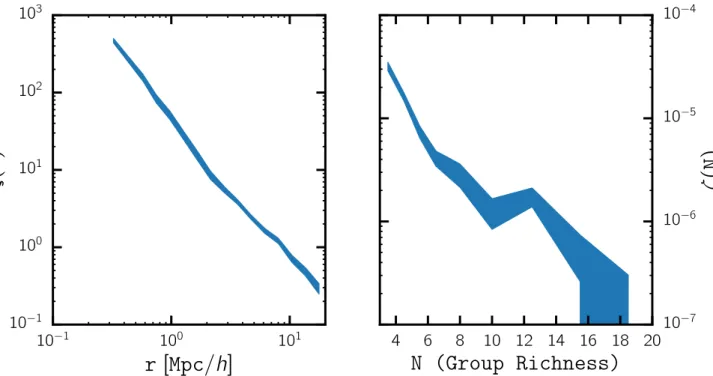
For our summary statistics of the catalogues, we use the mean

number density ¯ng, the galaxy two-point correlation functionξgg(r)

and the group multiplicity function_ζg(N). Our mock observation

catalogue has ¯ng=9.288 75×10−4h−3Mpc3, and in Fig.1, we

plot ξgg(r) (left-hand panel) and ζg(N) (right-hand panel). The

width of the shaded region represents the square root of the di-agonal elements of the summary statistic covariance matrix, which is computed as we describe below.

We calculateξggusing the natural estimator (Section 2.3) with 15

radial bins. The edges of the first radial bin are 0.15 and 0.5h−1Mpc.

The bin edges for the next 14 bins are logarithmically spaced

be-tween 0.5 and 20h−1Mpc. We compute the_ζg(N) as described in

Section 2.3 with nine richness bins, where the bin edges are loga-rithmically spaced between 3 and 20. To calculate the covariance matrix, we first run the forward model using the true HOD

parame-ters for all 125 halo catalogue subvolumes:{BOX1, ...,BOX125}. We

compute the summary statistics of each subvolume galaxy sample

k:

x(k)_{=[ ¯}

ng, ξgg, ζg], (13)

Figure 1. The two-point correlation functionξgg(r) (left) and group multiplicity functionζg(N) (right) summary statistics of the mock observations generated

from the ‘true’ HOD parameters described in Section 3.1. The width of the shaded region corresponds to the square root of the covariance matrix diagonal elements (equation 14). In our ABC analysis, we treat theξgg(r) andζg(N) above as the summary statistics of the observation.

Then we compute the covariance matrix as

Csample_i,j = 1 Nmocks−1

Nmocks

k=1

x(_ik)−x_i x(_jk)−x_j

, (14)

wherex_i = 1

Nmocks

Nmocks

k=1

x(_ik). (15)

Throughout our ABC-PMC analysis, we treat the ¯ng,ξgg(r) and

ζg(N) we describe in this section as if they were the summary

statistics of actual observations. However, we benefit from the fact that these observables are generated from mock observations using the true HOD parameters of our choice: we can use the true HOD parameters to assess the quality of the parameter constraints we obtain from ABC-PMC.

3.2 ABC-PMC design

In Section 2.1, we describe the key components of the ABC algo-rithm we use in our analysis. Now, we describe the more specific choices we make within the algorithm: the distance metric, the choice of priors, the distance threshold and the convergence

crite-ria. So far we have described three summary statistics: ¯ng,ξgg(r)

andζg(N). In order to explore the detailed differences in the

ABC-PMC parameter constraints based on our choice of summary

statis-tics, we run our analysis for two sets of observables: ( ¯ng,ξgg) and

( ¯ng,ζg).

For both analyses, we use a multicomponent distance (Silk,

Filippi & Stumpf2012, Cisewsky et al., in preparation). Each

sum-mary statistic has a distance associated with it:ρn,ρξ andρζ. We

calculate each of these distance components as

ρn=

¯ nd

g−n¯mg

2

σ2

n

, (16)

ρξ =

k

ξd

gg(rk)−ξggm(rk)

2

σ2

ξ,k

, (17)

ρζ =

k

ζd

g(Nk)−ζgm(Nk)

2

σ2

ζ,k

. (18)

The superscripts d and m denote the data and model, respectively. The data are the observables calculated from the mock observation

(Section 3.1).σ2

n,σ

2

ξ,kandσ

2

ζ,kare not the diagonal elements of the

covariance matrix (14). Instead, they are diagonal elements of the

covariance matrixCABC_.

We constructCABC_{by populating the entireMultiDarkhalo}

cat-alogues 125 times repeatedly, calculating ¯ng,ξgg andζgfor each

realization, and then computing the covariance associated with these

observables across all realizations. We highlight thatCABC_differs

from equation (14), in that it does not populate the 125 subvolumes

but the entireMultiDarksimulation and therefore does not

incorpo-rate sample variance. The ABC-PMC analysis instead accounts for the sample variance through the forward generative model, which populates the subvolumes in the same manner as the observations.

We use_σ2

n,σξ,k2 andσζ,k2 to ensure that the distance is not biased to

variations of observables on specific radial or richness bin.

For our ABC-PMC analysis using the observables ¯ngandξgg,

our distance metric isρ=[ρn, ρξ], while the distance metric for the

ABC-PMC analysis using the observables ¯ngandζgisρ=[ρn, ρζ].

To avoid any complications from the choice for our prior, we select uniform priors over all parameters aside from the scatter parameter

σlogM, for which we choose a log-uniform prior. We list the range

of our prior distributions in Table1.

With the distances and priors specified, we now describe the distance thresholds and the convergence criteria we impose in our analyses. For the initial iteration, we set distance thresholds for each

Table 1. Prior specifications. The prior probability distribu-tion and its range for each of the Zheng et al. (2007) HOD parameters. All mass parameters are in unit ofh−1_{M .}

HOD parameter Prior Range

α Uniform [0.8, 1.3]

σlog M Log-uniform [0.1, 0.7]

logM0 Uniform [10.0, 13.0]

logMmin Uniform [11.02, 13.02]

logM1 Uniform [13.0, 14.0]

distance component to∞. This means that the initial poolθ1is

simply sampled from the prior distribution we specify above. After the initial iteration, the distance threshold is adaptively lowered in subsequent iterations. More specifically, we follow the choice

of Lin & Kilbinger (2015) and set the distance threshold _t to

the median ofρ_t−1, the multicomponent distance of the previous

iteration of particles (θ_t−1).

The distance threshold_twill progressively decrease. Eventually

after a sufficient number of iterations, the region of parameter space

occupied byθ_twill remain unchanged. As this happens, the

accep-tance ratio begins to fall significantly. When the accepaccep-tance ratio drops below 0.001, our acceptance ratio threshold of choice, we deem the ABC-PMC algorithm as converged. In addition to the ac-ceptance ratio threshold we impose, we also ensure that distribution of the parameters converges – another sign that the algorithm has converged. Next, we present the results of our ABC-PMC analyses

using the sets of observables ( ¯ng,ξgg) and ( ¯ng,ζg).

3.3 Results: ABC

We describe the ABC algorithm in Section 2.1 and list the partic-ular choices we make in the implementation in the previous sec-tion. Finally, we demonstrate how the ABC algorithm produces parameter constraints and present the results of our ABC

analy-sis – the parameter constraints for the Zheng et al. (2007) HOD

model.

We begin with a qualitative demonstration of the ABC algorithm

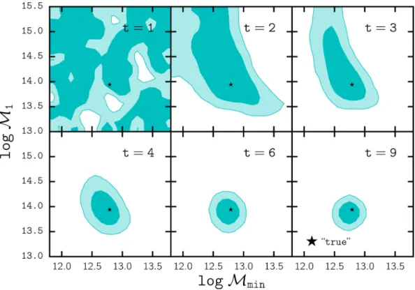
in Fig.2, where we plot the evolution of the ABCθ_tover the

iter-ationst=1–9, in the parameter space of [logM1,logMmin]. The

ABC procedure we plot in Fig.2uses ¯nandζg(N) for observables,

but the overall evolution is the same when we use ¯nandξgg(r). The

darker and lighter contours represent the 68 per cent and 95 per cent

confident regions of the posterior distribution overθ_t. For reference,

we also plot the ‘true’ HOD parameterθtrue(black star) in each of

the panels. The parameter ranges of the panels are equivalent to the

ranges of the prior probabilities we specify in Table1.

Fort=1, the initial pool (top left), the distance threshold1=

[∞,∞], soθ1uniformly samples the prior probability over the

parameters. At each subsequent iteration, the threshold is lowered

(Section 3), so fort_<6 panels, we note that the parameter spaced

occupied byθ_tdramatically shrinks. Eventually when the algorithm

begins to converge,t>7, the contours enclosing the 68 per cent and

95 per cent confidence interval stabilize. At the final iterationt=9

(bottom right), the algorithm has converged and we find thatθtrue

lies within the 68 per cent confidence interval of theθ_t=9particle

distribution. Thisθ_tdistribution at the final iteration represents the

posterior distribution of the parameters.

Figure 2. We demonstrate the evolution of the ABC particles,θt, over iterationst=1–9 in the logMminand logM1parameter space. ¯nandζg(N) are used

as observables for the above results. For reference, in each panel, we include the ‘true’ HOD parameters (black star) listed in Section 3.1. The initial distance threshold,1=[∞,∞] att=1 (top left), so theθ1spans the entire range of the prior distribution, which is also the range of the panels. We see fort<5, the

parameter space occupied by the ABCθtshrinks dramatically. Eventually when the algorithm converges,t>7, the parameter space occupied byθtno longer

shrinks and their distributions represent the posterior distribution of the parameters. Att=9, the final iteration, the ABC algorithm, has converged and we find thatθtruelies safely within the 68 per cent confidence region.

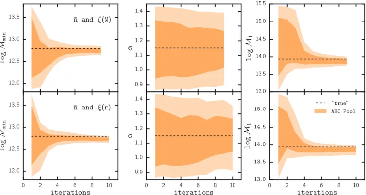
Figure 3. We illustrate the convergence of the ABC algorithm through the evolution of the ABC particle distribution as a function of iteration for parameters logMmin(left),α(centre) and logM1 (right). The top panel corresponds our ABC results using the observables ( ¯n, ζg(N)), while the lower panel plots

corresponds to the ABC results using ( ¯n, ξgg(r)). The distributions of parameters show no significant change aftert>7, which suggests that the ABC algorithm

has converged.

To better illustrate the criteria for convergence, in Fig. 3, we

plot the evolution of theθ_tdistribution as a function of iteration

for parameters logMmin(left),α(centre) and logM1(right). The

darker and lighter shaded regions correspond to the 68 per cent and

95 per cent confidence levels of theθ_tdistributions. The top panels

correspond to our ABC results using ( ¯n, ζg) as observables and the

bottom panels correspond to our results using ( ¯n, ξgg). For each

of the parameters in both top and bottom panels, we find that the

distribution does not evolve significantly fort>7. At this point,

additional iterations in our ABC algorithm will neither impact the

distance threshold_t nor the posterior distribution ofθ_t. We also

emphasize that the convergence of the parameter distributions co-incides with when the acceptance ratio, discussed in Section 3.2, crosses the predetermined shut-off value of 0.001. Based on these

criteria, our ABC results for both ( ¯n, ζg) and ( ¯n, ξgg) observables

have converged.

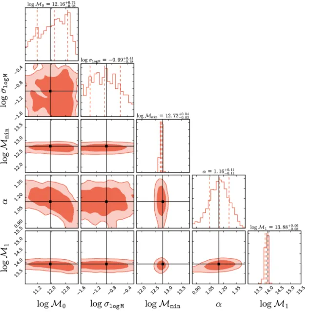
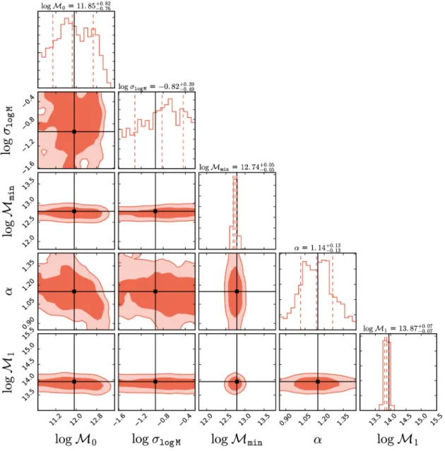
We present the parameter constraints from the converged ABC

analysis in Figs 4and 5. Fig.4shows the parameter constraints

using ¯nandξgg(r), while Fig.5plots the constraints using ¯nand

ζg(N). For both figures, the diagonal panels plot the posterior

dis-tribution of the HOD parameters with vertical dashed lines marking the 50 per cent (median) and 68 per cent confidence intervals. The off-diagonal panels plot the degeneracy between parameter pairs. To determine the accuracy of our ABC parameter constraints, we plot the ‘true’ HOD parameters (black) in each of the panels. For both sets of observables, our ABC constraints are consistent with

the ‘true’ HOD parameters. For logM0, logσlogMandα, the true

parameter values lie near the centre of the 68 per cent confidence in-terval. For the other parameter, which have much tighter constraints, the true parameters lie within the 68 per cent confidence interval.

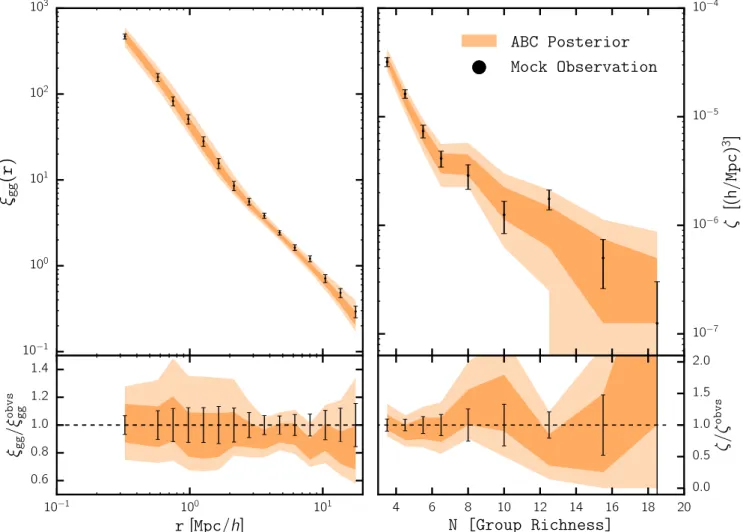
To further test the ABC results, in Fig.6, we compare ξgg(r)

(left) andζg(N) (right) of the mock observations from Section 3.1

to the predictions of the ABC posterior distribution (shaded). The error bars of the mock observations represent the square root of the diagonal elements of the covariance matrix (equation 14), while the darker and lighter shaded regions represent the 68 per cent and 95 per cent confidence regions of the ABC posterior predictions. In the lower panels, we plot the ratio of the ABC posterior

pre-dictionξgg(r) and ζg(N) over the mock observationξggobvs(r) and

ζobvs

g (N). Overall, the ratio of the 68 per cent confidence region of

ABC posterior predictions is consistent with unity throughout the

rand Nrange. We observe slight deviations in the ξgg ratio for

r> 5 Mpc/h; however, any deviation is within the uncertainties

of the mock observations. Therefore, the observables drawn from the ABC posterior distributions are in good agreement with the observables of the mock observation.

The ABC results we obtain using the algorithm of Section 2.1 with the choices of Section 3.2 produce parameter constraints that

are consistent with the ‘true’ HOD parameters (Figs4and5). They

also produce observablesξgg(r) andζg(N) that are consistent with

ξobvs

gg andζgobvs. Thus, through ABC we are able to produce consistent

parameter constraints. More importantly, we demonstrate that ABC is feasible for parameter inference in LSS.

3.4 Comparison to the Gaussian pseudo-likelihood MCMC analysis

In order to assess the quality of the parameter inference described in the previous section, we compare the ABC-PMC results with the HOD parameter constraints from assuming a Gaussian likeli-hood function. The model used for the Gaussian likelilikeli-hood analy-sis is different than the forward generative model adopted for the ABC-PMC algorithm to be consistent with the standard approach.

Figure 4. We present the constraints on the Zheng et al. (2007) HOD model parameters obtained from our ABC-PMC analysis using ¯nandξgg(r) as observables.

The diagonal panels plot the posterior distribution of each HOD parameter with vertical dashed lines marking the 50 per cent quantile and 68 per cent confidence intervals of the distribution. The off-diagonal panels plot the degeneracies between parameter pairs. The range of each panel corresponds to the range of our prior choice. The ‘true’ HOD parameters, listed in Section 3.1, are also plotted in each of the panels (black). For logM0,αandσlogM, the ‘true’ parameter

values lie near the centre of the 68 per cent confidence interval of the posterior distribution. For logM1and logMmin, which have tight constraints, the ‘true’

values lie within the 68 per cent confidence interval. Ultimately, the ABC parameter constraints, we obtain in our analysis are consistent with the ‘true’ HOD parameters.

In the ABC analysis, the model accounts for sample variance by randomly sampling a subvolume to be populated with galaxies. Instead, in the Gaussian pseudo-likelihood analysis, the covariance matrix is assumed to capture the uncertainties from sample variance. Hence, in the model for the Gaussian pseudo-likelihood analysis,

we populate haloes of theentireMultiDarksimulation rather than

a subvolume. We describe the Gaussian pseudo-likelihood analysis below.

To write down the Gaussian pseudo-likelihood, we first introduce

the vectorx: a combination of the summary statistics (observables)

for a galaxy catalogue. When we use ¯ngandξgg(r) as observables in

the analysis:x=[ ¯ng, ξgg]; when we use ¯ngandζg(N) as observables

in the analysis:x=[ ¯ng, ζg]. Based on this notation, we can write

pseudo-likelihood function as

−2 lnL(θ|d)=xT_C−1_x+ln[(2π)d_{det(C)], (19)}

where

x=[xobs−xmod], (20)

the difference betweenxobs, measured from the mock observation

and xmod(θ) measured from the mock catalogue generated from

the model with parameters θ. dhere is the dimension of x (for

x=[ ¯ng, ξgg],d=13; forx=[ ¯ng, ζg],d=10).C−1is the inverse

covariance matrix, which we estimate following Hartlap, Simon &

Figure 5. Same as Fig.4but for our ABC analysis using ¯nandζg(N) as observables. The ABC parameter constraints we obtain are consistent with the ‘true’

HOD parameters.

Schneider (2007):

C−1= Nmocks−d−1 Nmocks−1

C−1. (21)

C is the estimated covariance matrix, calculated using the

corre-spondingxblock of the covariance matrix from equation (14) and

Nmockis the number of mocks used for the estimation (Nmock=124;

see Section 3.1). We note that in_Cthe dependence on the HOD

pa-rameters is neglected, so the second term in the expression of equa-tion (19) can be neglected. Finally, using this pseudo-likelihood, we sample from the posterior distribution given the prior distribution

using the MCMC sampleremcee(Foreman-Mackey et al.2013).

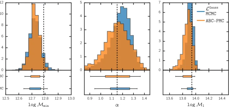
In Figs7and8, we compare the results from ABC-PMC and

Gaussian pseudo-likelihood MCMC analyses using [ ¯ng, ξgg] and

[ ¯ng, ζg] as observables, respectively. The top panels in each figure

compares the marginalized posterior PDFs for three parameters of

the HOD model:{logMmin, α,logM1}. The lower panels in each

figure compares the 68 per cent and 95 per cent confidence intervals of the constraints derived from the two inference methods as a box

plot. The ‘true’ HOD parameters are marked by vertical dashed lines in each panel.

In both Figs 7and 8, the marginalized posteriors for each of

the parameters from both inference methods are comparable and consistent with the ‘true’ HOD parameters. However, we note that there are minor discrepancies between the marginalized

poste-rior distributions. In particular, the distribution forαderived from

ABC-PMC is less biased than theαconstraints from the Gaussian

pseudo-likelihood approach.

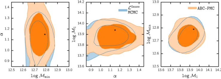
In Figs9and10, we plot the contours enclosing the 68 per cent

and 95 per cent confidence regions of the posterior probabilities of

the two methods using [ ¯ng, ξgg] and [ ¯ng, ζg] as observables,

respec-tively. In both figures, we mark the ‘true’ HOD parameters (black star). The overall shape of the contours is in agreement with each other. However, we note that the contours for the ABC-PMC method

are more extended alongα.

Overall, the HOD parameter constraints from ABC-PMC are consistent with those from the Gaussian pseudo-likelihood MCMC method; however, using ABC-PMC has a number of advantages.

Figure 6. We compare the ABC-PMC posterior prediction for the observablesξgg(r) (left) andζg(N) (right) (orange; Section 3.3) toξgg(r) andζg(N) of the

mock observation (black) in the top panels. In the lower panels, we plot the ratio between the ABC-PMC posterior predictions forξggandζgto the mock

observationξobvs

gg andζgobvs. The darker and lighter shaded regions represent the 68 per cent and 95 per cent confidence regions of the posterior predictions,

respectively. The errorbars represent the square root of the diagonal elements of the error covariance matrix (equation 14) of the mock observations. Overall, the observables drawn from the ABC-PMC posteriors are in good agreement withξggandζgof the mock observations. The lower panels demonstrate that for

both observables, the error-bars of the mock observations lie within the 68 per cent confidence interval of the ABC-PMC posterior predictions.

For instance, ABC-PMC utilizes a forward generative model. Our forward generative model accounts for sample variance. On the other hand, the Gaussian pseudo-likelihood approach, as mentioned earlier this section, does not account for sample variance in the model and relies on the covariance matrix estimate to capture the sample variance of the data.

Accurate estimation of the covariance matrix in LSS, however, faces a number of challenges. It is both labour and computation-ally expensive and dependent on the accuracy of simulated mock catalogues, known to be unreliable on small scales (see Heitmann

et al.2008; Chuang et al.2015and references therein). In fact,

as Sellentin & Heavens (2016) points out, using estimates of the

covariance matrix in the Gaussian psuedo-likelihood approach be-come further problematic. Even when inferring parameters from a Gaussian-distributed data set, using covariance matrix estimates

rather than thetruecovariance matrix leads to a likelihood

func-tion that isno longerGaussian. ABC-PMC does not depend on a

covariance matrix estimate; hence, it does not face these problems. In addition to not requiring accurate covariance matrix esti-mates, forward models of the ABC-PMC method, in principle, also have the advantage that they can account for sources of systematic

uncertainties that affect observations. All observations suffer from significant systematic effects that are often difficult to correct. For

instance, in SDSS-III BOSS (Dawson et al.2013), fibre collisions

and redshift failures significantly bias measurements and analysis

of observables such as ξgg or the galaxy power spectrum (Guo,

Zehavi & Zheng2012; Ross et al.2012; Hahn et al.2017). In

pa-rameter inference, these systematics can affect the likelihood, and thus any analysis that requires writing down the likelihood, in un-known ways. With a forward generative model of the ABC-PMC method, the systematics can be simulated and marginalized out to achieve unbiased constraints.

Furthermore,ABC-PMC – unlike the Gaussian pseudo-likelihood

approach – is agnostic about the functional form of the underlying distribution of the summary statistics(e.g.ξggandζg). As we

ex-plain throughout the paper, the likelihood function in LSScannotbe

Gaussian. Forξgg, the correlation function must satisfy non-trivial

positive-definiteness requirements and hence the Gaussian pseudo-likelihood function assumption is not correct in detail. In the case

ofζg(N), assuming a Gaussian functional form for the likelihood,

which in reality is more likely Poisson, misrepresents the true like-lihood function. In fact, this incorrect likelike-lihood may explain why

Figure 7. We compare the logMmin,αand logM1parameter constraints from ABC-PMC (orange) to constraints from the Gaussian pseudo-likelihood

MCMC (blue) using ¯ngandξgg(r) as observables. The top panels compares the two methods’ marginalized posterior PDFs over the parameters. In the bottom

panels, we include box plots marking the confidence intervals of the posterior distributions. The boxes represent the 68 per cent confidence interval, while the ‘whiskers’ represent the 95 per cent confidence interval. We mark the ‘true’ HOD parameters with vertical black dashed line. The marginalized posterior PDFs obtained from the two methods are consistent with each other. The ABC-PMC and Gaussian pseudo-likelihood constraints are generally consistent for logMmin

and logM1. The ABC-PMC constraint forαis slightly less biased and has slightly larger uncertainty then the constraint from Gaussian pseudo-likelihood

analysis.

Figure 8. Same as Fig.7, but both the ABC-PMC analysis and the Gaussian pseudo-likelihood MCMC analysis use ¯ng andζg(N) as observables. Both

methods derive constraints consistent with the ‘true’ HOD parameters and infer the region of allowed values to similar precision. We note that the MCMC constraint onαis slightly more biased compared to ABC-PMC estimate. This discrepancy may stem from the fact that the use of Gaussian pseudo-likelihood and its associated assumptions is more spurious when modelling the group multiplicity function.

the constraints onαare less biased for the ABC-PMC analysis than

the Gaussian-likelihood analysis in Fig.10.

Although in our comparison using simple mock observations, we find generally consistent parameter constraints from both the ABC-PMC analysis and the standard Gaussian pseudo-likelihood analysis, more realistic scenarios present many factors that can

generate inconsistencies. Consider a typical galaxy catalogue from LSS observations. These catalogues consist of objects with differ-ent data qualities, signal-to-noise ratios and systematic effects. For example, catalogues are often incomplete beyond some luminos-ity/redshift or have some threshold signal-to-noise ratio cut imposed on them.

Figure 9. We compare the ABC-PMC (orange) and the Gaussian pseudo-likelihood MCMC (blue) predictions of the 68 per cent and 95 per cent posterior confidence regions over the HOD parameters (logMmin,αand logM1) using ¯ngandξgg(r) as observables. In each panel, the black star represents the ‘true’

HOD parameters used to generate the mock observations. Both inference methods derive confidence regions consistent with the ‘true’ HOD parameters.

Figure 10. Same as Fig.9, but using ¯ngandζg(N) as observables. Again, the confidence regions derived from both methods are consistent with the ‘true’

HOD parameters used to generate the mock observations. The confidence region ofαfrom the Gaussian pseudo-likelihood method is biased compared to the ABC-PMC contours. This may be due to the fact that the true likelihood function that describesζg(N) deviates significantly from the assumed Gaussian

functional form.

These selection effects, coupled with the systematic effects earlier this section, make correctly predicting the likelihood intractable. In the standard Gaussian pseudo-likelihood analysis, and other analy-sis that require writing down a likelihood function, these effects can significantly bias the inferred parameter constraints. In these situa-tions, employing ABC equipped with a generative forward model that incorporates selection and systematic effects may produce less biased parameter constraints.

Despite the advantages of ABC, one obstacle for adopting it to parameter inference has been the computational costs of generative forward models, a key element of ABC. By combining ABC with the PMC sampling method, however, ABC-PMC efficiently converges to give reliable posterior parameter constraints. In fact, in our anal-ysis, the total computational resources required for the ABC-PMC

analysis werecomparableto the computational resources used for

the Gaussian pseudo-likelihood analysis with MCMC sampling. Applying ABC-PMC beyond the analysis in this work, to broader LSS analyses, imposes some caveats. In this work, we focus on the galaxy–halo connection, so our generative forward model populates haloes with galaxies. The LSS analyses for inferring cosmological

parameters would require generating haloes by running cosmologi-cal simulations. The forward models also need to accurately model the observation systematic effects of the latest observations. Hence, accurate generative forward models in LSS analyses demand im-provements in simulations and significant computational resources in order to infer unbiased parameter constraints. Recent cosmology simulations show promising improvements in both accuracy and

speed (e.g. Feng et al.2016). Such developments will be crucial

for applying ABC-PMC to broader LSS analyses and exploiting the significant advantages that ABC-PMC offers.

4 S U M M A RY A N D C O N C L U S I O N

Approximate Bayesian Computation, ABC, is a generative, simulation-based inference that can deliver correct parameter es-timation with appropriate choices for its design. It has the advan-tage over the standard approach in that it does not require explicit knowledge of the likelihood function. It only relies on the ability to simulate the observed data, accounting for the uncertainties asso-ciated with observation and on specifying a metric for the distance

between the observed data and simulation. When the specification of the likelihood function proves to be challenging or when the true underlying distribution of the observable is unknown, ABC provides a promising alternative for inference.

The standard approach to LSS studies relies on the assumption that the likelihood function for the observables – often two-point correlation function – given the model has a Gaussian functional form. In other words, it assumes that the statistical summaries are Gaussian distributed. In principle to rigorously test such an as-sumption, a large number of realistic simulations would need to be generated in order to examine the actual distribution of the ob-servables. This process, however, is prohibitively – both labour and computationally – expensive. Therefore, our assumption of a Gaussian likelihood function remains largely unconfirmed and so unknown. Fortunately, the framework of ABC permits us to bypass any assumptions regarding the distribution of observables. Through ABC, we can provide constraints for our models without making the unexamined assumption of Gaussianity.

With the ultimate goal of demonstrating that ABC is feasible for the LSS studies, we use it to constrain parameters of the halo occupation distribution, which dictates the galaxy–halo connection. We begin by constructing a mock observation of galaxy distribution with a chosen set of ‘true’ HOD model parameters. Then, we attempt to constrain these parameters using ABC. More specifically, in this paper,

(i) we provide an explanation of the ABC algorithm and present how Population Monte Carlo can be utilized to efficiently reach convergence and estimate the posterior distributions of model pa-rameters. We use this ABC-PMC algorithm with a generative

for-ward model built withHALOTOOLS, a software package for creating

catalogues of galaxy positions based on models of the galaxy–halo connection such as the HOD;

(ii) we choose ¯ng,ξggandζgas observables and summary

statis-tics of the galaxy position catalogues. And for our ABC-PMC algo-rithm, we specify a multicomponent distance metric, uniform priors, a median threshold implementation and an acceptance rate-based convergence criterion;

(iii) from our specific ABC-PMC method, we obtain parameter constraints that are consistent with the ‘true’ HOD parameters of our mock observations. Hence, we demonstrate that ABC-PMC can be used for parameter inference in the LSS studies;

(iv) we compare our ABC-PMC parameter constraints to con-straints using the standard Gaussian-likelihood MCMC analysis. The constraints we get from both methods are comparable in

ac-curacy and precision. However, for our analysis using ¯ngand ζg

in particular, we obtain less biased posterior distributions when comparing to the ‘true’ HOD parameters.

Based on our results, we conclude that ABC-PMC is able to consistently infer parameters in the context of LSS. We also find that the computation required for our ABC-PMC and standard Gaussian-likelihood analyses are comparable. Therefore, with the statistical advantages that ABC offers, we present ABC-PMC as an improved alternative for parameter inference.

AC K N OW L E D G E M E N T S

We thank Jessie Cisewsky for reading and making valuable com-ments on the draft. We would also like to thank Michael R. Blanton, Jeremy R. Tinker, Uros Seljak, Layne Price, Boris Leidstadt, Alex Malz, Patrick McDonald and Dan Foreman-Mackey for produc-tive and insightful discussions. MV was supported by NSF grant

AST-1517237. DWH was supported by NSF (grants IIS-1124794 and AST-1517237), NASA (grant NNX12AI50G) and the Moore-Sloan Data Science Environment at NYU. KW was supported by NSF grant AST-1211889. Computations were performed us-ing computational resources at NYU-HPC. We thank Shenglong Wang, the administrator of NYU-HPC computational facility, for his consistent and continuous support throughout the development of this project. We would like to thank the organizers of the

Astro-HackWeek 2015 workshop (http://astrohackweek.org/2015/), since

the direction and the scope of this investigation was – to some de-gree – initiated through discussions in this workshop. Throughout this investigation, we have made use of publicly available

soft-ware packages EMCEE and ABCPMC. We have also used the

pub-licly availablePYTHONimplementation of the FoF algorithmpyfof

(https://github.com/simongibbons/pyfof).

R E F E R E N C E S

Akeret J., Refregier A., Amara A., Seehars S., Hasner C., 2015, J. Cosmol. Astropart. Phys., 8, 043

Ata M., Kitaura F.-S., M¨uller V., 2015, MNRAS, 446, 4250

Beaumont M. A., Cornuet J.-M., Marin J.-M., Robert C. P., 2009, Biometrika, 96, 983

Behroozi P. S., Wechsler R. H., Wu H.-Y., 2013a, ApJ, 762, 109 Behroozi P. S., Wechsler R. H., Conroy C., 2013b, ApJ, 770, 57 Berlind A. A., Weinberg D. H., 2002, ApJ, 575, 587

Berlind A. A. et al., 2006, ApJS, 167, 1

Bernardeau F., Colombi S., Gazta˜naga E., Scoccimarro R., 2002, Phys. Rep., 367, 1

Bishop C., 2007, Pattern Recognition and Machine Learning (Information Science and Statistics), 1st edn. Springer-Verlag, New York

Bond J. R., Cole S., Efstathiou G., Kaiser N., 1991, ApJ, 379, 440 Cacciato M., van den Bosch F. C., More S., Mo H., Yang X., 2013, MNRAS,

430, 767

Cameron E., Pettitt A. N., 2012, MNRAS, 425, 44

Casas-Miranda R., Mo H. J., Sheth R. K., Boerner G., 2002, MNRAS, 333, 730

Chuang C.-H. et al., 2015, MNRAS, 452, 686 Conroy C., Wechsler R. H., 2009, ApJ, 696, 620 Cooray A., Sheth R., 2002, Phys. Rep., 372, 1

Davis M., Efstathiou G., Frenk C. S., White S. D. M., 1985, ApJ, 292, 371 Dawson K. S. et al., 2013, AJ, 145, 10

Del Moral P., Doucet A., Jasra A., 2006, J. R. Stat. Soc. B, 68, 411 Dressler A., 1980, ApJ, 236, 351

Dutton A. A., Macci`o A. V., 2014, MNRAS, 441, 3359 Eriksen H. K. et al., 2004, ApJS, 155, 227

Feng Y., Chu M.-Y., Seljak U., McDonald P., 2016, MNRAS, 463, 2273 Filippi S., Barnes C., Stumpf M., 2011, preprint (arXiv:1106.6280) Foreman-Mackey D., Hogg D. W., Lang D., Goodman J., 2013, PASP, 125,

306

Guo H., Zehavi I., Zheng Z., 2012, ApJ, 756, 127

Hahn C., Scoccimarro R., Blanton M. R., Tinker J. L., Rodr´ıguez-Torres S., 2017, MNRAS, 467, 1940

Hartlap J., Simon P., Schneider P., 2007, A&A, 464, 399 Hearin A. et al., 2016a, preprint (arXiv:1606.04106)

Hearin A. P., Zentner A. R., van den Bosch F. C., Campbell D., Tollerud E., 2016b, MNRAS, 460, 2552

Heitmann K. et al., 2008, Comput. Sci. Discovery, 1, 015003

Heitmann K., Higdon D., White M., Habib S., Williams B. J., Lawrence E., Wagner C., 2009, ApJ, 705, 156

Heitmann K., White M., Wagner C., Habib S., Higdon D., 2010, ApJ, 715, 104

Ishida E. E. O., Vitenti S. D. P., Penna-Lima M., Cisewski J., de Souza R. S., Trindade A. M. M., Cameron E., Busti V. C., 2015, Astron. Comput., 13, 1

Kaiser N., 1984, ApJ, 284, L9