CAS: Capital Framework for Property Liability Insurers

Capital Framework for

Property Liability Insurers

by Zia Rehman

ABSTRACT

Experience shows that U.S. risk-based capital measures do not

always signal financial troubles until it is too late. Here we

pre-sent an alternative, reasonable capital adequacy model that can be

easily implemented using data commonly available to company

actuaries. The model addresses the three most significant risks

common to property and casualty companies—namely,

pric-ing, interest rate, and reserving risk. Both row and column effects

are incorporated into the model. Rating agencies, company

man-agement, U.S. regulators, and European Solvency II regulators all

represent parties who should find this model useful. We suggest

revision of charges pertaining to these risks in the risk-based

capi-tal formula. The framework also provides loss reserve uncertainty

and margins under IASB accounting standards and net capital

estimation, which is useful when considering reinsurance

pro-gram consequences. European Solvency II regulations require a

one-year forward distribution of ultimate losses, which is easily

obtained. The model is applicable to all lines where triangulation

of data is feasible, including health and group life insurance.

KEYWORDS

ter of 2008, and more than $1 billion in the previous four quarters (Triad Business Journal 2008). More-over, when United Guaranty reorganized, it chose to reinsure business written between 2005–2008 to get it off of their books, suggesting that United Guaranty’s troubles did not happen overnight, but instead over a period of several years, culminating in 2008 (England 2012). Yet on July 9, 2008, Moody’s Investor Service notes, “For UGRIC’s mortgage insurance portfolio overall, capital adequacy on a risk-adjusted basis is consistent with Moody’s double-A metrics, and the company is currently well within regulatory limits” (Moody’s Investors Service 2008). Also the North Carolina Insurance Department did not take regula-tory action until United Guaranty’s capital adequacy problems were well known, and AIG had all but col-lapsed. AIG was able to get a capital infusion and chose to “save” United Guaranty, but many other pri-vate mortgage insurance (PMI) companies did not fare as well during the 2008 financial crisis. For example, Triad Guaranty Insurance Corporation also collapsed, and is now winding down as it placed its business in run-off. If RBC were truly an effective indicator, one would have expected it to indicate the possibility of financial troubles sooner.

Most of those studying the topic agree that RBC results present several shortcomings as a way of mod-eling capital adequacy. Likewise, no agreement exists in the literature about the best way to model capital on a going-concern basis, the basis of most interest to investors, for example.

In this paper, we focus on capital modeling issues. Our purpose is to develop a reasonable capital ade-quacy model that can be easily implemented using data commonly available to company actuaries. The flexible framework provided can be adapted to meet the needs of rating agencies, company management, and regulators. Our capital adequacy model is also compatible with European Solvency II’s risk-based economic capital framework.

The paper proceeds in the following way. In the section that follows, we preface model development by suggesting alternative ways of defining pricing

1. Introduction

The question of whether a property/casualty insur-ance company possesses sufficient capital to continue operating remains one of the most important problems faced by insurance regulators, rating agencies, and company management. The National Association of Insurance Commissioners (NAIC) relies in part upon risk-based capital standards to ensure that a company’s capital remains adequate to support current and past writings. Using conservative statutory accounting val-uations, the risk-based capital requirements give reg-ulators a tool to use in justifying prompt regulatory action against a troubled company, action which does not require a court order and helps limit the effect of a potential insolvency (Lewis 1998). Risk-based capi-tal (RBC) results might also be employed by a rating agency as one measure of an insurance company’s financial strength. Yet many times the tool simply has not worked as envisioned, with capital inadequacy not indicated by RBC until it was too late.

quar-Interest rate risk. Most models calculate the vari-ability of portfolio returns on an asset-by-asset basis and then aggregate the risk. Instead, the risk is the mis-match between investment income offset which under-lies rates, and the actual interest income earned on loss reserves and on (the loss portion of) unearned premium reserves. Also, aggregating the risk usually requires measuring a correlation matrix and that introduces measurement errors due to the many extra param-eters that are hard to estimate.

Interdependence.All risks are related through

time and are not independent. Many researchers model these three risks separately and then combine them using a correlation matrix. This often requires normal-ity assumptions that are hard to justify in practice. Fur-ther, as is the case with interest rate risk, this usually requires measuring a correlation matrix and that intro-duces measurement errors due to many extra param-eters that are hard to estimate. The schematic flow of risks for a 12-month policy year is shown below:

Time = 1 Time = 2 Time = 3 Time = Maturity

Pricing risk Reserving &Pricing, Interest risk

Reserving & Interest rate

risk

Losses paid: no risk

A 12-month policy year spans two accident years and losses from these two incurred accident years lead to uncertainty in loss reserves (reserving risk). The unearned premium and loss reserves are invested at all times and result in interest rate risk. Pricing risk vanishes after 24 months, once all premiums are earned and all losses are incurred. Thus “risks” are correlated at different times. In this paper we model them together, without any explicit assumption of the correlations between them.

Discussion.The current literature on capital

model-ing does not address the concerns we raise above. In addition, there is currently no consensus on the sto-chastic methods used to determine capital. For a com-prehensive review of existing methods, the reader is referred to Goldfarb (2006).

There are also many papers that deal with the sub-set of risks that underlie capital. For example, reserv-ing risk is discussed in many papers (e.g., see Mach risk and interest rate risk that better capture the risks

presented by these two aspects of RBC. These risks, combined with reserving risk, cannot be treated as independent, and thus we model them together without making assumptions about the correlations between them. Section three includes a framework that links to company reserves and can be updated as needed to accommodate both different reserve parameters and new data. The fourth section presents a two-effects (row and column) model, including postulates and two theorems, while section five applies the model to common capital measures of value at risk and condi-tional value at risk. A few applications of the model are presented in section six. The seventh and final section concludes the paper.

2. Capital modeling deficiencies

Of the risks considered by most capital adequacy models, pricing, reserving, and interest rate risk seem most important to most property/casualty insurance companies. We examine definitions of these below.

Pricing risk.This refers to the risk that actual losses differ from those anticipated in the rates. Contrary to common perception, the nature of risk faced by insur-ance companies is not the underlying losses. It is the mismatch between loss provision in rates and the actual losses. Traditional capital models fail to capture this risk due to their focus on underlying losses and their distributions.1

Reserving risk.This refers to the risk due to

vari-ability in loss reserves. Many models calculate capital levels due to reserving risk with the assumption that a certain method was used to set these reserves. In practice, reserves can be hand selected. Regardless of the methods used to select reserves, the reserving risk must be captured. Many models work well for certain methods of calculating reserves while actuaries often use a combination of models as well as judgment (Rehman and Klugman 2010).

1_{Such mismatch was severe in the case of PMI industry due to}

the square root rule +

∑

=

C Ck

k n

.

0 2

1

Here,C_k refers to the capital charge due to riskk.We limit our attention to the three largest risks for most property casualty insurance companies, namely, interest rate risk, pric-ing risk, and reservpric-ing risk. Our framework presents a different way of calculating charges for these three risks, with the following four caveats in mind: • We ignore the interest rate risk due to capital charges

themselves. In other words, we assume that capital itself is placed in the safest possible investment. This assumption can be removed, and the risk incorporated into the model, but we chose not to do so for the sake of simplicity.

• All data used to measure risk charges comes from rate filings and annual statements. For example, we use implied link ratios based on held reserves (schedule P Part 2) and not indicated reserves (see Appendix A). These link ratios are used to build data triangles, discussed more completely in section 3.3. • To build insurance risk triangles, we need actual

portfolio returns by calendar year. Under SAP accounting, these equate to realized portfolio returns. • Instead of three charges, a single charge is

calcu-lated and replaced in the RBC formula.

3.2. Economic capital: GAAP accounting

In accordance with “going concern” accounting treatment, the insurance risk triangles rely upon indi-cated link ratios. Portfolio returns, also employed in building insurance risk triangles, reflect both real-ized and unrealreal-ized gains. We again ignore interest rate risk associated with economic capital itself, just as we did with respect to risk capital above.

Also under GAAP accounting, the company should combine capital charges due to other risks (e.g., credit risks) into calculated capital. In most property casu-alty insurance companies, such charges are typically a much smaller part of total capital. Hence, we do not discuss them further.

Moving forward, our discussion will be common to both types of capital. One can obtain risk capital versus economic capital by simply modifying the dataset. Therefore, we will only use the term “capital” 1993). These models are often the basis of capital

cal-culation. As mentioned earlier, these papers calculate reserving risk for a particular type of reserving model while actual reserves are likely hand selected and based on the many different methods deployed.

3. Capital framework

In this section, we set forth a framework for estimat-ing required capital. The framework includes a model that links to company reserves and can be updated as needed to accommodate both different reserve param-eters and new data. This pragmatic approach fits easily with an actuarial department’s reserving framework.

We consider two versions of the model: an SAP-based2 _{model for insurance regulators, and a} GAAP-based3 _{capital model useful for internal company} management and rating agencies. The respective accounting treatments do influence model results, which is why it is important to incorporate them into our discussions. We do that explicitly in sec-tions 3.1 and 3.2.

Before proceeding, we note that for solvency pur-poses, the “required capital” derived under the two different accounting treatments can each be com-pared to the company’s balance sheet held capital.

3.1. Risk capital: SAP accounting

The risk-based capital (RBC) formula explicitly incorporates six main risk charges (see Feldblum 1996).4_{These charges are combined additively using}

2_{The acronym SAP refers to Statutory Accounting Practices, accounting}

rules that consider valuations on a “solvency” basis for insurance regula-tory purposes. As compared to GAAP, valuations derived under SAP may be lower, and thus, more conservative than those derived using GAAP.

3_{The acronym GAAP refers to Generally Accepted Accounting}

Princi-ples, accounting rules that consider valuations on a “going concern” basis.

4_{The charges include off-balance sheet risks and risks from insurance}

amount earned over time. At time 0, the insurance company receives premium income, which becomes earned as losses are incurred over the life of the policy. Once all losses incur and premiums become earned, unearned premium reserves for a given policy year go to 0, and pricing risk disappears. Thus the first column of Table 1 is always the UEPR of respective policy years and represents the best estimate of the losses at that time.6 _{This estimate} changes over time due to incurred losses.

• Reserving risk: Allocate direct accident year losses, by age, to each policy year. Develop them to mate using incurred accident year age to ulti-mate development factors. These are then added to the UEPR at each respective age. In this man-ner we state the revised estimates of policy year ultimate losses at each age.

• Interest rate risk: Begin by recognizing that interest rates impact diagonal values only. Next, we need two additional quantities, namely, the investment income offset that underlies rates due to policyholder sup-plied funds (by policy year) and the actual earned portfolio interest rate underlying unearned premium and loss reserves. If the actual interest rate proves higher than expected, we decrease the diagonal to reflect the added investment income. The converse is also true. This way, all the diagonals become restated. The last diagonal remains unchanged, since no data for actual interest rate is available at this point. Thus, henceforth. We now present the data structure for

non-catastrophic lines, and a complete discussion of adjust-ments needed to put them into catastrophic insurance risk triangles will follow.

3.3. Data structure: Non-catastrophic

insurance risk triangles

In Table 1, data is available forM (fixed) policy yearsi= 2, 3 . . .M.Thus row entries in the table can be obtained by varyingi. However, for any fixedM

the quantityU_M-i+1 provides only the last (diagonal) column entry for row i.The value on the adjacent diagonal would beU_M-i. We do not introduce a vari-able for the realized part of the rectangle, as our inter-est lies in the unknown (missing) cells of the policy yeari, and we will be contented with just naming the values by their specific symbols in the realized part. The unrealized part, referenced by adding a subscript,

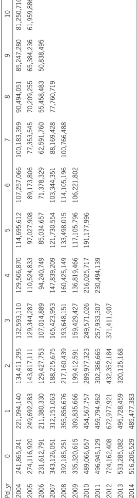
q= 1, 2 . . . i- 1, such thatU_M-i+1+q now references future cells for rowi.We explain below the steps to prepare the dataset for any policy year (i.e., the real-ized part). We jointly model interest rate, pricing, and reserving risks by capturing them in a single data triangle. Prepare the insurance risk triangle, shown in Table 1, which consists of company’s “estimates” of ultimate lossesUitracked on a policy year basis, by adding the following components:

• Pricing risk: Let (1-expense load)* written premium= trimmed unearned premium reserves (UEPR),5_an

6_{Under SAP accounting, we would not use trimmed UEPR and use the}

full written premium as UEPR. Table 1. Insurance risk triangle: [Më M+ 1]

0 1 2 . . . M-i M-i+ 1 . . . M-i M

1 U1,0 U1,1 U1,2 . . . U1,M-i U1,M-i+1 . . . U1,M-1 U1,M

2 U2,0 U2,1 U2,2 . . . U2,M-i U2,M-i+1 . . . U2,M-1

3 U3,0 U3,1 U3,2 . . . U3,M-i U3,M-i+1 . . .

. . . .

i Ui,0 Ui,1 Ui,2 Ui,M-i Ui,M-i+1

i+ 1 Ui+1,0 Ui+1,1 Ui+1,2 Ui+1,M-i . . .

M UM,0 UM,1

5_{UEPR: We do not subtract the profit load (= underwriting profit}

tility in these ratios reflects the insurance risk faced when writing the underlying policies. Larger absolute values of the natural log ratios imply greater deviations from previous estimates. Signs associated with errors also may prove informative. For example, a finding of negative policy year cumulative errors would imply rate redundancy for the policy year.

Note that the insurance risk triangles depend on charged premiums. They include any market adjust-ments present in the loss costs underlying rate indi-cations, such as schedule rating credits/debits or experience rating modifications.

The non-catastrophe insurance risk and error tri-angles described above can be constructed using data commonly available to actuaries. Companies wishing to determine economic capital and rating agencies could prepare them for this purpose. Hence, these tri-angles prove very pragmatic from an implementation perspective.

From a practical standpoint, insurance risk triangles are not available in annual statements. This is not a shortcoming of the framework, since the true risk faced by an insurance company is on a policy-year basis because it is always “older” than accident year. Current capital models often ignore the lag between the two due to the fact that Schedule P is compiled on an accident year basis and it’s easier to compile data using accident year than mapping losses on a policy-year basis. For precisely this reason, the capital requirements fall short when the lag is significant— especially in lines with significant pricing risk such as property catastrophe. For lines where pricing risk is insignificant, such as auto physical damage and auto since the final diagonal remains unchanged, interest

rate risk adds uncertainty to cash flow timing only. In GAAP accounting, capital gains/losses are part of the calculation of “actual earned interest income” underlying insurance risk triangles. For example, if a bond portfolio underlying loss reserves decreases in value due to increase in interest rates, the decrease in value will lower the actual return on the policy-holder–supplied funds and thus affect the diagonals of the insurance risk triangles.

Another issue is related to the investment income offset. The offset is set in advance for a policy year and cannot be changed. For example, using new money yields on policyholder supplied funds will affect the actual portfolio return but not the invest-ment income offset itself.

We assume that the triangle of errors contains all policy years underlying the economic cycle con-templated in the return period. Further, the loss data should be available until maturity for those policy years. Define:

U_i,M-i+1= Insurance Risk amount for policy yeari, esti-mated at development ageM-i+ 1

e_i,M-i+1 = Error for policy year i and development interval (M-i, M-i+ 1)

=

− + − +

−

e U

U i M i i M i

i M i

ln .

, 1 , 1

,

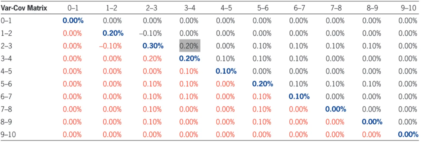
Below the Insurance Risk triangle presented in Table 1, find a triangle of errors,e_i in Table 2 that indi-cates the extent of under- or over-pricing. The

vola-Table 2. Error triangle: [Më M]

1 2 . . . M-i M-i+ 1 . . . M- 1 M

1 e1,1 e1,2 . . . e1,M-i ei,M-i+1 . . . e1,M-1 e1,M

2 e2,1 e2,2 . . . e2,M-i e2,M-i+1 . . . e2,M-1

. . . .

i ei,1 ei,2 . . . ei,M-i ei,M-i+1

i+ 1 ei+1,1 ei+1,2 . . . ei+1,M-i

. . . .

are independent of other non-catastrophic events, the dollar losses may not be independent due to macro and micro economic variables, such as inflation. It is also possible that geographies may create a rela-tionship between catastrophic and non-catastrophic losses simply due to different construction standards. A univariate analysis ignores such covariance effects or at least makes assumptions in quantifying them.

For the rest of the paper, we will assume non-catastrophic insurance risk triangles with the under-standing that catastrophic losses can be incorporated into the model.

3.5. Discussion: Insurance risk triangle

In the section above, we consider how to construct insurance risk triangles and error triangles. Other variations exist, and we would like to devote atten-tion to two of these, as well as to reflecatten-tions on under-writing cycles, before proceeding to a case study.

Instead of using incurred losses, we can use paid losses to construct insurance triangles. When paid losses are used we must use accident year paid ulti-mate loss development factors as opposed to incurred factors.7_{The use of paid versus incurred depends on} the company’s situation. If the company sets case reserves in a reasonable way, then incurred data should be used, as it accurately reflects the company’s reserving situation.

Instead of using direct written premiums and losses to make insurance risk and error triangles, net written premiums and losses may be employed, resulting in a net insurance risk triangle. For such triangles we also use net age to ultimate factors from net reserve reviews. Use of direct or net insurance risk triangles will lead to direct or net capital.

We now turn our attention to the issue of underwrit-ing cycles embedded in the data. If the data contain a complete underwriting cycle (peak and trough) then the parameters measured from those data will encode the strength of the cycle. The data triangles used in liability, one can build insurance risk triangles using

accident year basis and ignore pricing risk (approxi-mation). Hence, pragmatically, regulators may limit data calls in the form of insurance risk triangles only from companies suspected to be in trouble or lines of business that have high pricing risk. This discussion ties back to statements we made in section 3.1.

3.4. Incorporating catastrophic losses

Catastrophic losses refer to hit-and-miss events such as hurricanes, where usual triangulation of data would leave missing values. Hence, tornadoes may be non-catastrophic in states such as Iowa where these occur each year but the same would be catastrophic in Maine where they are rare. With this definition, we now show adjustments needed to non-catastrophic insurance risk triangles in order to reflect catastrophic risk:

(1) Catastrophic models should be used to determine losses on current exposures due to actual (not modeled) historical catastrophes. This will pro-vide the company with a long enough history of data that captures cycles of such rare events. Still, in many calendar years, one would expect no loss. (2) These losses must be combined with non-catastrophic losses to produce a “total” insur-ance risk triangle. The non-catastrophic losses should have the same number of years of policy year history as catastrophic losses. This ensures that there are no missing values in the triangle, although in some calendar years we would have “spikes” due to actual catastrophic losses. (3) The starting expected loss (Figure 1, time 0)

includes charges for catastrophes.

There are several advantages of this model over the current practice of determining capital for cata-strophic losses separately and combining it with non-catastrophic losses. First, it considers errors due to pricing versus actual historical experience. This is in contrast to using modeled losses to determine capi-tal. Second, the model is multivariate and considers covariance effects between catastrophic versus non-catastrophic losses. Even if catastrophes themselves

7_{Another variation includes using quarterly as opposed to annual policy}

3.7. Case study

We end section 3 by presenting data for line X. The purpose of the case study is to help illustrate key computational ideas described earlier in section 3.3, as well as throughout the rest of the paper. As a prac-tical matter, for variance/covariance calculation pur-poses, an extra row is needed to ensure that the last age (the last column in the triangle) has at least two data points. ThusM= 10 and the policy year 2004 is the extra row added.

4. Two effects model

Real-world changes often take place on a calendar year basis. In Tables 1 and 2, the diagonals represent calendar years. It is clear that any “calendar year effect” will result in dependence of both policy years (rows) and columns (development periods). From a mathe-matical perspective, we cannot appeal to independence arguments. Instead, we will develop our model with recognition of both policy year (row effect) and devel-opment interval (column effect) dependencies.

We present two distinct approaches to capital mea-surement. The first, value at risk (VaR), provides a percentile measure of risk tolerance. It requires capital to be set so that there isa probability of insolvency. The second, conditional value at risk (CVaR), specifies risk tolerance at a given conditional expected excess loss. The condition here is typically the VaR loss amount. Hence, CVaR is always more conservative than VaR for the same specified percentilea. Conditional value at risk possesses a property of risk measures known as coherence (see Artzner, Delbaen, et al. 1999), implying compliance with a set of commonsense axioms. Value at risk, lacking this property, can lead to perverse con-sequences in some circumstances.

4.1. Model postulates

Table 2, the error triangle, presents half of the val-ues present in a rectangle, the observed half, with the rest of the values considered unobserved. Since our randomness is due to unobserved values, we ignore this paper will assume that at least one complete

underwriting cycle has been observed. All param-eters estimated from this data will make the model

relative to this fact: the number of underwriting cycles in the data.

Suppose that we are concerned with future under-writing cycles impacting past business written on a policy-year basis. Future underwriting cycles can be driven by several factors, such as changes in laws, external market competition, and the external busi-ness environment (e.g., inflationary pressures). Com-monly, actuaries adjust for future cyclical effects by incorporating ancillary data. Our methodology per-mits a way to readily incorporate such data.

3.6. Industry data

For capital modeling purposes, it’s not correct to use industry data. It makes sense to combine esti-mates using credibility if the estiesti-mates are measuring the same quantity. In a capital measurement context, the company’s data is a result of its unique exposures, geography and other variables. Industry parameters are based on a different data set. Also, a low volume of data8 _{of the company is not a problem but rather a} reality that must impact parameter estimates. Third, the confidence intervals of the parameter estimates involving sample means and variances have reason-ably low standard errors due to the strong law of large numbers.

In cases where a complete triangle is not available, such as a company with a rapidly changing busi-ness mix for a given line or a new company with no data, the only option may be ad hoc approaches such as using parameters of a peer company of a similar size. However, it’s never feasible to apply industry fac-tors and “adjust” them to a particular company when company-specific data is available. Similarly, industry “factors” can be calculated based on the model and applied to all companies, but such an approach would not be recommended.

8_{We still require a complete triangle of data but for each policy year there}

This postulate proves unnecessary later, when we use additional data. Hence, we relax it below in sub-section 4.4 when we present Theorem 2, but retain it for Theorem 1, presented in subsection 4.3.

4.2. Column effect: dependence

of development periods

Given our postulates,k= 1, 2 . . .i- 1

e U

U N

i M i k i M i k i M i k

i M i k i M i k

ln ,

, 1 , 1

,

, 1 2, 1

∼

(

)

= µ σ

− + + − + +

− + − + + − + +

Thus, each future entry in the error triangle in Table 2 is postulated as marginally normally dis-tributed and the parameters vary by both rows and columns. In the context of capital, half the rectangle is observed and we are interested in the randomness due to the remaining half of unobserved normally dis-tributed error values.

For column effects, we will keep the policy yeari

fixed and sum over the unobservedk= 1, 2 . . .i- 1 errors

∑

∑

( )

= = =

= ∗

− + + =

= −

− + +

− + =

= −

− +

− +

e e U

U

U U

U U e

i i M i k k

k i

i M i k

i M i k k

k i

i M

i M i

i M i M i i

ln ln

exp (1)

, 1 1

1

, 1 , 1

1

, , 1

, , 1

Note thatU_i,M is an unknown final policy year ulti-mate loss, whileU_i,M-i+1 is fixed and known. Due to the normality assumption,

Table 2’s first row, as it is assumed to be complete.9 We postulate that the unobserved errors {e_i,M-i+1}_2≤i≤M are multivariate normally distributed.10 _{Additionally,} for estimation purposes, we make the following two assumptions about Table 2:

(i) For any given column, the errors have the same marginal variance. This assumption permits the use of a sample variance as an estimate of the marginal population variance.

(ii) Pairs of errors in any two columns have the same covariance. This permits the use of a sample cova-riance as an estimate of the population covacova-riance. The last two postulates are necessary for calibra-tion of the parameters. However, note the following caveats. First, sample estimates should be updated as new data emerges each year. Second, the old “completed rows” from the insurance risk triangle in Table 1 greatly enhance accuracy in estimation and should be retained. We note a third postulate since it will be used to derive Theorem 1:

(iii) For any given column, the errors have the same marginal mean. This permits the use of a sample mean as an estimate of the population mean.

Table 4. Error triangle

Log Ratio 0–1 1–2 2–3 3–4 4–5 5–6 6–7 7–8 8–9 9–10

2004 -9.0% -49.8% -1.4% -2.4% -12.1% -6.7% -6.8% -10.2% -6.0% -4.8%

2005 -9.3% -55.2% -10.6% -15.7% -13.0% -8.4% -14.2% -9.7% -7.1% -5.4%

2006 -9.1% -49.1% -19.0% -12.7% -10.3% -17.5% -13.1% -12.1% -8.7%

2007 -9.5% -50.6% -12.9% -11.2% -19.4% -16.4% -15.9% -12.6%

2008 -9.7% -49.4% -11.5% -18.8% -18.4% -15.7% -12.4%

2009 -7.9% -44.1% -22.4% -15.3% -15.6% -9.8%

2010 -7.3% -45.0% -15.0% -14.4% -12.2%

2011 -7.8% -41.9% -15.9% -11.2%

2012 -7.3% -44.2% -15.2%

2013 -7.3% -43.7%

2014 -6.1%

9_{Adding extra rows will later help in estimation (especially for late}

devel-opment periods with few entries in columns) as we will estimate quanti-ties using columns in Table 2.

10_{The theoretical rationale for this is discussed in Rehman and Klugman}

values from Table 2. Thus

∑

µ − + + =

= −

i M i k k

k i

, 1 1

1

accumulates these means for future development periods for a given policy year i. Table 7’s cumulative column shows the results.

e N

e e

i

i M i k k

k i

i i M i k i M i l

l l i

k k i

,

cov ,

(2)

, 1 1

1

2

, 1 , 1

1 1 1

1

∼

∑

∑

∑

(

)

µ

σ = 

    



     − + +

= = −

− + + − + + =

= −

= = −

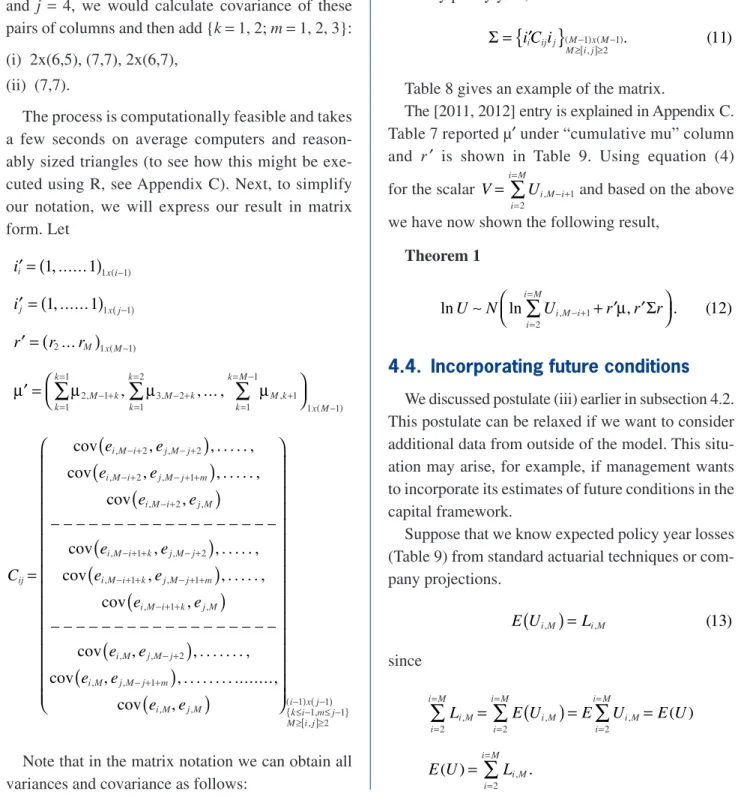
For a fixed i the “column covariance matrix,” namely {cov(e_i,M-i+k+1,e_i,M-i+l+1)}_k,l;k, l∈{1, 2 . . .i- 1} can be estimated using the observed half rectangle of errors (Table 2). The result is shown in Table 5.

For example, the (2–3, 3–4) entry is calculated using Table 4 and taking covariance of columns:

Error 2–3 3–4

2004 -1.4% -2.4%

2005 -10.6% -15.7%

2006 -19.0% -12.7%

2007 -12.9% -11.2%

2008 -11.5% -18.8%

2009 -22.4% -15.3%

2010 -15.0% -14.4%

2011 -15.9% -11.2%

2012 -15.2%

Covariance 0.2%

Note thats2

2014 is the sum of all entries in Table 5 except 0–1 row/column;s2

2013 is the sum of all entries after deleting the first two rows and columns, etc. Table 6 shows these results.

Similarly, for a fixedi, the error means µ_i,M-i+k+1 can be estimated by averaging each column of observed

Table 5. Column covariance matrix

Var-Cov Matrix 0–1 1–2 2–3 3–4 4–5 5–6 6–7 7–8 8–9 9–10

0–1 0.00% 0.00% 0.00% 0.00% 0.00% 0.00% 0.00% 0.00% 0.00% 0.00%

1–2 0.00% 0.20% -0.10% 0.00% 0.00% 0.00% 0.00% 0.00% 0.00% 0.00% 2–3 0.00% -0.10% 0.30% 0.20% 0.00% 0.10% 0.10% 0.10% 0.10% 0.00% 3–4 0.00% 0.00% 0.20% 0.20% 0.10% 0.10% 0.10% 0.00% 0.00% 0.00% 4–5 0.00% 0.00% 0.00% 0.10% 0.10% 0.00% 0.00% 0.00% 0.00% 0.00% 5–6 0.00% 0.00% 0.10% 0.10% 0.00% 0.20% 0.10% 0.10% 0.10% 0.00% 6–7 0.00% 0.00% 0.10% 0.10% 0.00% 0.10% 0.10% 0.00% 0.00% 0.00% 7–8 0.00% 0.00% 0.10% 0.00% 0.00% 0.10% 0.00% 0.00% 0.00% 0.00% 8–9 0.00% 0.00% 0.10% 0.00% 0.00% 0.10% 0.00% 0.00% 0.00% 0.00% 9–10 0.00% 0.00% 0.00% 0.00% 0.00% 0.00% 0.00% 0.00% 0.00% 0.00%

Table 6. Variances

PY Variance

2014 3.30%

2013 3.30%

2012 1.80%

2011 1.00%

2010 0.90%

2009 0.10%

2008 0.00%

2007 0.00%

2006 0.00%

2005 0.00%

Table 7. Estimation of error means

PY Error Mean Cumulative

2006 -5.09% -5.09%

2007 -7.26% -12.35%

2008 -11.13% -23.49%

2009 -12.50% -35.98%

2010 -12.41% -48.40%

2011 -14.43% -62.83%

2012 -12.73% -75.56%

2013 -13.76% -89.32%

HereV is the sum of observed values along the diagonal of the insurance risk triangle (Table 1) for all open years and the weights are the relative proportion in each policy year. If the error random variables e_i

are close to zero, consider the following Taylor series approximations:

e U

V r e r e

r e r e

i i i i M i i i i M i i i i M i i i i M

ln ln exp ln 1

ln 1 .

2 2 2 2

∑

∑

∑

∑

( ) ( ) = =    ≈ +     =  +  ≈ = = = = = = = =

The approximate log-ratio has a normal distribu-tion and, thus, U has an approximate lognormal dis-tribution. The variance of the normal distribution is

Var U

V Var i r ei i r r e e i M

i j i j i

i M

j j M

ln cov , .

(6)

2 2 2

∑

∑

∑

( )

≈ _ _{ =}

(

)

= = = = = = From (2), E U

V E i r ei i r E e r i M

i i i

i i M

i i M

i M i k k

k i

ln .

(7)

2 2 2 1 , 1

1

∑

∑

∑

∑

( )

_{≈ } _{ =} ( )= µ

= = = = = = − + + = = − Now,

r r e e

r Var e r r e e

i j i j i

i M

j j M

i i i j i j

j j M

i j

cov ,

2 cov , . (8)

column

effect effectrow

2 2 2 2

∑

∑

∑

∑

(

)

(

)

( ) = + ← ←→ → = = = = = = <

The estimation ofVar(e_i) was discussed under col-umn effect. The second term is due to dependence of policy years (row effect). For 2≤i <j and using (1),

∑

∑

∑

∑

(

)

(

)

= _ _ = − + + = = − − + + = = − − + + − + + = = − = = −

e e e e

e e

i j i M i k

k k i

j M j m m

m j

i M i k j M j m m

m j

k k i

cov , cov ,

cov , . (9)

, 1 1 1 , 1 1 1

, 1 , 1

1 1 1

1 From (1) sinceU_i,M-i+1 is considered fixed,U_i,M will

have a lognormal distribution,

U

U N

e e

i M

i M i

i M i k k

k i

i M i k i M i l l l i k k i ln , cov , , , 1 , 1 1 1

, 1 , 1

1 1 1 1 ∼

∑

∑

∑

(

)

µ             − + − + + = = − − + + − + + = = − = = − U N U e e i M

i M i i M i k k

k i

i M i k i M i l l l i k k i ln ln , cov , (3) ,

, 1 , 1

1 1

, 1 , 1

1 1 1 1 ∼

∑

∑

∑

(

)

+ µ             − + − + + = = − − + + − + + = = − = = −

The above follows from (2). We can therefore esti-mate the policy year distribution.

4.3. Row effect: Dependence

of policy years

Our goal is to sum across all policy years and determine the distribution of

U Ui M i i M . , 2

∑

= = =

SinceU_i,M is lognormal, we have a sum of log-normal random variables. There is no closed form dis-tribution forU but simulation techniques can be used to determine the exact distribution (Appendix B). We provide closed-form results in this section that are approximations. These approximations are generally quite good. From (1), the total loss for all policy years can be written as

∑

∑

( ) = = ∗ = = − + = =

U Ui M U e

i i M

i M i i i M i exp , 2 , 1 2

∑

( ) = = =

U V ri e

i i M i exp 2

∑

= − + = =

V Ui M i i i M (4) , 1 2

∑

= − + − + = = r U U i i M i

j M j j

j M (5)

i j M

e ei j i C ii ij j

2 , ,

cov

(

,

)

. (10)

[ ]

(

≤ ≤

)

= ′

The above bilinear form simply sums up all ele-ments of matrixC_ij. This form is convenient since wheni=j we get variances. Putting this information in a matrix form gives us the covariance matrix of errors by policy year,

i C ii ij j M x M

M i j1, 2 1. (11)

{

}

Σ = ′

[ ]

( −) ( −) ≥ ≥

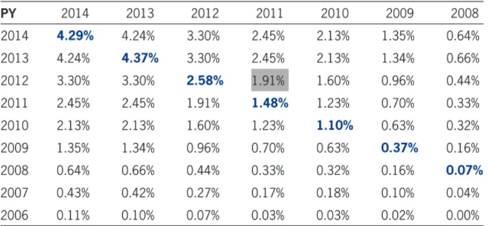
Table 8 gives an example of the matrix.

The [2011, 2012] entry is explained in Appendix C. Table 7 reported µ′ under “cumulative mu” column and r′ is shown in Table 9. Using equation (4) for the scalar =

∑

− +

= =

V Ui M i i

i M , 1 2

and based on the above we have now shown the following result,

Theorem 1

U N Ui M i r r r

i i M

ln ln , 1 , . (12)

2

∼ _

∑

− + + ′µ ′Σ _ =

=

4.4. Incorporating future conditions

We discussed postulate (iii) earlier in subsection 4.2. This postulate can be relaxed if we want to consider additional data from outside of the model. This situ-ation may arise, for example, if management wants to incorporate its estimates of future conditions in the capital framework.

Suppose that we know expected policy year losses (Table 9) from standard actuarial techniques or com-pany projections.

(

)

=

E Ui M, Li M, (13) since

L E U E U E U

E U L

i M i M

i i M i i M i M i i M i M i i M . , , 2

2 2 ,

, 2

∑

∑

∑

∑

(

)

( ) ( ) = = = = = = = = = = = =

The covariance matrix {cov(e_i,M-i+k+1, e_j,M-j+m+1)}_k,m is not square and hence we cannot assume any sym-metry. Similar to the estimation ofVar(e_i), the double sum is over the unobserved values and can be esti-mated from the error triangle (Table 2) using column data. For fixedi, j we need to calculate the sum of all possible covariance betweenfuturecolumns of these policy years. To illustrate ifM= 8, for policy yearsi= 3 and j = 4, we would calculate covariance of these pairs of columns and then add {k= 1, 2;m= 1, 2, 3}: (i) 2x(6,5), (7,7), 2x(6,7),

(ii) (7,7).

The process is computationally feasible and takes a few seconds on average computers and reason-ably sized triangles (to see how this might be exe-cuted using R, see Appendix C). Next, to simplify our notation, we will express our result in matrix form. Let

∑

∑

∑

(

)

(

)

(

)

′ = ′ = ′ = ′

µ =_ µ µ µ _

( ) ( ) ( ) ( ) − − − − + = = − + + = = − = = − i i

r r r

i x i

j x j

M x M

M k k

k

M k M k

k k M k k x M 1, ...1 1, ...1 ... , , ... , 1 1 1 1

2 1 1

2, 1 1 1

3, 2 , 1

1 1 1 2 1 1

(

)

(

)

(

)

(

)

(

)

(

)

(

)

(

)

(

)

=                                     [ ] ( ) { } ( ) − + − + − + − + + − + − + + − + − + + − + + − + + − + − + + − − ≤ − ≤ − ≥ ≥ C e e e e e e e e e e e e e e e e e e ij

i M i j M j

i M i j M j m

i M i j M

i M i k j M j

i M i k j M j m

i M i k j M

i M j M j

i M j M j m

i M j M i_{k i}x j_{m j} M i j

cov , , . . . , cov , , . . . ,

cov ,

– – – – – – – – – – – – – – – – – – cov , , . . . , cov , , . . . ,

cov ,

– – – – – – – – – – – – – – – – – – cov , , . . . , cov , , . . . ...,

cov ,

, 2 , 2 , 2 , 1

, 2 ,

, 1 , 2 , 1 , 1

, 1 ,

, , 2 , , 1

, , 1 _1, 1 ₁

Theorem 2, since in practical cases

∑

= =

Li M i i M

, 2

is available.

(ii) The variance component r′Sr is based on his-torical data alone and changes only as the data changes. In the actuarial and regulatory con-texts, this situation will usually happen once a year when the model is updated.

5. Capital measurement

The aforementioned property of coherence makes the CVaR approach appealing. However, the VaR lacks this property, laying the user open to counter-productive choices in capital management. This short-coming seems important to mention because of VaR’s widespread use, as well as the fact that its use is man-dated by some proposed regulatory régimes.

5.1. Value at risk (VaR) capital

Using (12), we define

∑

= _ − ′Σ + −α ′Σ _

= =

UVaR L r r z r r

i M i i M

: exp ln

2 (15)

, 1

2

H:= Held loss reserves11+ Held unearned premium reserves (line) + Policy year cumulative paid loss to date

I := Future investment income on held loss and unearned premium reserves

N11

We mentioned in Section (2) the usefulness of incor-porating future conditions in the capital framework. Here

∑

= =

Li M i i M

, 2

provides a way to incorporate these beliefs. Based on the above we have now shown the following result:

Theorem 2

∑

θ = − ′Σ ω = ′Σ



 ₌ 

=

∼

U N Li M r r r r

i i M

ln ln

2 , (14)

, 2

2

The above is justified, since

Li M r r r r L E U

i i M

i M i i M

exp ln

2 2 .

,

2 2 ,

∑

− ′Σ + ′Σ

∑

( )



 ₌  = =

=

= =

Comments:

(i) The use of Theorem 2 alleviates the need to estimate the vector µ. Henceforth we will use

Table 8. Covariance matrix by policy year

PY 2014 2013 2012 2011 2010 2009 2008

2014 4.29% 4.24% 3.30% 2.45% 2.13% 1.35% 0.64%

2013 4.24% 4.37% 3.30% 2.45% 2.13% 1.34% 0.66%

2012 3.30% 3.30% 2.58% 1.91% 1.60% 0.96% 0.44%

2011 2.45% 2.45% 1.91% 1.48% 1.23% 0.70% 0.33%

2010 2.13% 2.13% 1.60% 1.23% 1.10% 0.63% 0.32%

2009 1.35% 1.34% 0.96% 0.70% 0.63% 0.37% 0.16%

2008 0.64% 0.66% 0.44% 0.33% 0.32% 0.16% 0.07%

2007 0.43% 0.42% 0.27% 0.17% 0.18% 0.10% 0.04%

2006 0.11% 0.10% 0.07% 0.03% 0.03% 0.02% 0.00%

Table 9. Expected policy year losses

PY Reported Factor Ultimate r

2006 50,838,495 0.99 50,330,111 2.6%

2007 77,760,719 1.01 78,538,326 4.0%

2008 100,766,488 1.02 102,781,818 5.2%

2009 106,221,802 1.06 112,595,111 5.5%

2010 191,177,996 1.08 206,472,236 9.9%

2011 230,494,139 1.10 253,543,552 11.9%

2012 371,411,907 1.19 441,980,170 19.2%

2013 320,125,168 1.20 384,150,202 16.6%

2014 485,477,383 1.36 660,249,241 25.1%

be a distribution for each line separately and one for the combined lines, too. The fact that data is “less volatile” in the sense of lower sample variances obtained from the data is not a “problem” but a reality that in many cases the company faces lower volatility in its overall loss experience than any single line. In cases where a line’s mix is changing rapidly, it’s pos-sible to simulate ultimate losses (for all policy years) for that line and then combine it using covariance matrix. We do not provide details in the paper but the calculations are similar to Appendix B. Beliefs about future development of losses on these policy years can be incorporated through

∑

= =

Li M i i M

, 2

while emerging data will capture estimation of variance parameters.

5.3. Capacity

Capacity:= Sum of individual line capital- Total capital for all lines combined

Thus, capacity results from diversification across lines. Positive capacity lowers the capital requirement of the company and thus enhances solvency.

5.4. Conditional value at risk

(CVaR) capital

The capital can also be measured as a function of conditional expected cost in excess of a given dol-lar amountd.This is called conditional value at risk (CVaR) capital and is a more general case of tail value at risk (TVaR) capital, which requires a certain The full value capital under VaR is given by

CVaR_:=UVaR_{− −}H I_{. (16)}

Note that the future investment income on held loss and unearned premium reserves should be done at the appropriate interest rate. For risk-based capi-tal, we would use SAP accounting rules and for eco-nomic capital, we would use GAAP accounting rules. In both cases, we would use the current asset mix.

We assume that capital gets invested in risk-free assets. To find discounted capital, we discount using the risk-free rate and the duration determined from the insurance risk triangle. This duration reflects the runoff of both loss reserves and unearned premium reserves.

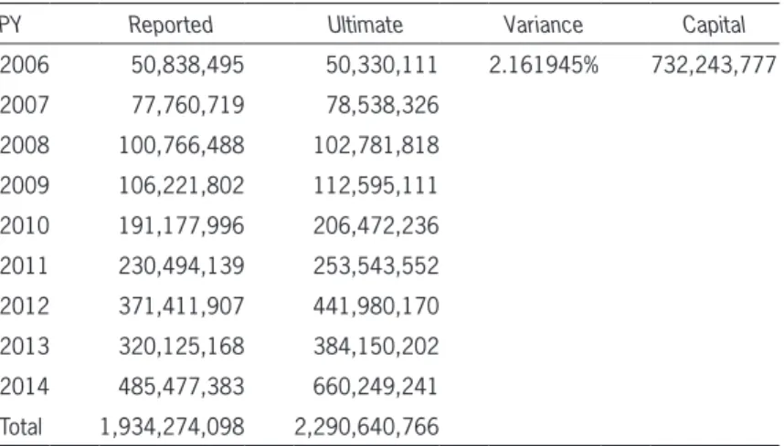
The undiscounted capital calculation (z_1-a=1.96) is shown in Table 10, where we have not subtractedI.

The capital is sensitive to the variance parameter. In particular, smaller companies/lines will generate larger variances and larger capital requirements.

5.2. Value at risk (VaR) capital

for multiple lines

Suppose that there are two lines of business. Each can be analyzed separately using the method previ-ously outlined. However, it is likely that the results for the lines are not independent.

We can combine the data (losses in Table 1) from the two lines into a single triangle and analyze it using the methods of this paper. When finished, there will

Table 10. Capital calculation

PY Reported Ultimate Variance Capital

2006 50,838,495 50,330,111 2.161945% 732,243,777

2007 77,760,719 78,538,326

2008 100,766,488 102,781,818

2009 106,221,802 112,595,111

2010 191,177,996 206,472,236

2011 230,494,139 253,543,552

2012 371,411,907 441,980,170

2013 320,125,168 384,150,202

2014 485,477,383 660,249,241

the ultimate loss. This can be obtained by noting that one-year forward means thatk=m= 1 and the matrix

C_ij reduces to a scalar.

There are no “fixed” models prescribed in Sol-vency II and a model can be filed for approval. The current model has several advantages. First, it pro-vides a nice way to measure “1 year” risk which is key to Solvency II. Second, the model ties back to reserve reviews, which is important to regulators. Third, the model is mathematically justified, sim-ple to understand and applicable across all types on property liability insurers (including niche lines such as private mortgage insurance) which is also impor-tant to regulators. The last point is imporimpor-tant, as no special models have to be created for niche lines.

6.2. Loss reserve uncertainty

The model presented represents an enhancement of Rehman and Klugman (2010) where accident years were assumed to be independent. To see the connec-tion with our model, suppose instead of using insur-ance risk triangles we used accident year triangles where diagonals are ultimate selected losses. Under SAP, these will be Schedule P Part 2 (includes bulk and IBNR reserves) while for GAAP, these will come from historical company reserve reviews.

In this case, the data contains only reserving risk, which means that capital is only due to this single source of risk. Theorems 1 and 2 will provide the dis-tribution ofU.The mean ofU in Theorem 1 has an interesting interpretation in this case. It corrects the “biases” of the actuary when selecting the ultimate losses. Once the parameters qandware known, we can determine the following measures:

Reserve margins. Under International

Account-ing Standards Board (IASB) reserve margins are now required. These margins consist of amounts or cush-ions above held capital amounts. Using CVaR and choice of d explained below. Note that, as a

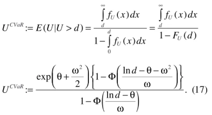
con-sequence of the positive lognormal support, U≥ 0. Using the CVaR definition,

U E U U d

f x dx

f x dx

f x dx

F d

U

d

d CVaR

U d

U d

U d

U

CVaR

:

1 1

: exp

2 1

ln

1 ln

. (17)

0

2 2

∫

∫

∫

(

)

( )

( )

( )

( )

( )

= > =

−

= −

=

θ + ω 

  − Φ

− θ − ω ω 

 

  

  

− Φ − θ

ω

∞ ∞

For a givend the above denotes the stress value of the loss for all policy years combined. Extension to multiple lines can be accomplished using the total company-wide data. The approach is similar to VaR.

= − −

CCVaR_: UCVaR H I ₍₁₈₎

To illustrate, supposed is based on VaR-based per-centileUVaR _{given by equation (15). This special case} of CVaR is called TVaR and is more conservative than VaR,

d UVaR L r z r r

i M i i M

exp ln

2 . (19)

, 2

1

∑

= = _ − ′Σ + ′Σ _

= =

−α

A comparison of VaR versus CVaR capital for the same parameters is given in Table 11.

6. Applications

The model presented is versatile and rich in appli-cations to other important areas. We discuss some of these below.

6.1. European Solvency II regulation

European regulation for insurance companies (Sol-vency II) requires a one-year forward distribution of

Table 11. Capital comparison

Approach q w2 _{Capital (dollars) Stress level}

VaR 21.5413 2.161945% 732,243,777 a = 5%

relations between them. We present a two-effects (row and column) model, including postulates and two theorems, as well as common capital measures of value at risk and conditional value at risk.

We follow our discussion of model development with mention of three significant applications: Euro-pean Solvency II regulation, loss reserve uncertainty and margins under IASB accounting standards— which generalizes the work of Rehman, Klugman (2010), and net capital estimation, which is useful when considering reinsurance program consequences. European Solvency II regulations require a one-year forward distribution of ultimate losses, easily obtained using the model.

The current approach would have resulted in much higher capital requirements for PMI companies, such as AIG United Guaranty. It is due to inherent historical volatility in housing data where home prices undergo a “bad patch” for several years in a row—often region-ally and result in extremely large loss ratios for PMI companies. The “bad patch” leads correlated years of losses and the traditional models as well as RBC underestimate this “effect.” Coupled with this, PMI have significant pricing risk as premiums are earned over a long period of time13 _{and the insurance risk} tri-angle will capture this pricing risk. In traditional acci-dent year models, this pricing risk would be ignored and hence cause underestimation of true risk.

Current risk-based capital frameworks used by U.S. insurance regulators and rating agencies often fail to signal capital deficiency problems until it is too late. In this paper, we propose an alternative model that relies on data commonly available to actuaries. The framework allows for a modified calculation of risk-based capital amounts under statutory accounting rules, as well as the computation of economic capi-tal amounts using going concern accounting rules. Thus, it should be useful to companies, regulators, and rating agencies alike. The model accommodates the European Solvency II framework as well. VaR approaches described above, we can determine

the stress value of U. Equation (16) is modified in this case:

H:= Held loss reserves12_{+Accident year} cumula-tive paid loss to date.

The full value reserve margin under VaR is given by CVaR_:=UVaR₋H_{. (20)}

Reserve confidence intervals.These are obtained

from the confidence interval ofU minus cumulative paid losses.

6.3. Net capital

Net capital:= Direct capital- Ceded capital.

If the VAR approach is used to set capital, thenza for the direct and ceded analysis should be the same. Likewise, for the CVaR,d should be calculated using a consistent percentile.

An alternative to the above approach is to conduct a net analysis directly using net written premiums and net losses in the data step. In that case, the net capital can be estimated directly.

7. Conclusion

In this paper, we develop a reasonable capital ade-quacy framework that can be easily implemented using data commonly available to company actuaries. The flexible framework provided can be adapted to meet the needs of rating agencies, company management and regulators and updated along with annual reserve reviews. Our capital adequacy model is also compati-ble with European Solvency II’s risk-based economic capital framework.

Our framework captures pricing risk, interest rate risk and reserving risk more accurately than RBC risk charges and we recommend replacing current cal-culation of RBC risk charges. These risks cannot be treated as independent, and thus we model them together without making assumptions about the

cor-12_{Use indicated reserves under GAAP.}

13_{Policyholder pays premiums as long as the mortgage stays and loan to}

Mack, T., “Distribution-free Calculation of the Standard Error of Chain Ladder Reserve Estimates,”ASTIN Bulletin, 1993, pp. 213–225.

Moody’s Investors Service, “Rating Action: Moody’s Downgrades United Guaranty to Aa3; Outlook is Negative,” New York: Moody’s Corporation, July 9, 2008.

RBC Dependencies and Calibration Working Party (DCWP), Solvency II Standard Formula and NAIC Risk-Based Capi-tal (RBC), Report 3 of the CAS Risk Based CapiCapi-tal (RBC) Research Working Parties,Casualty Actuarial Society E-Forum,

Fall 2012, pp. 1–38.

Rehman, Z., and S. Klugman, “Quantifying Uncertainty in Reserves,”Variance, 2010, pp. 30–46.

Triad Business Journal,AIG United Guaranty Parent Replaces CEO. Retrieved March 28, 2015, Triad Business Journal: June 16, 2008, www.bizjournals.com/triad/stories/2008/06/16/ daily1.html.

Acknowledgments

We are indebted to Lisa Gardner (Professor, Drake University) for her help with the introduction and literature review of the paper. Lisa also proofread the document and made valuable suggestions.

Appendix A. Calculating Implied

Link Ratios

When the selected ultimate losses and the incurred triangle are given the implied link ratios can be gleaned from the data.

Example

AQ 3 6 9 12 SelectedUltimate

2000 Q1 100 120 180 200 200

2000 Q2 120 160 200 250

2000 Q3 150 200 300

2000 Q4 200 400

Solution:

Development to Age

Intervals Ultimate FactorImplied Age to DevelopmentIntervals Implied AgeLink Ratio

3–Ult 400/200= 2.00 3–6 2/1.5= 1.33

6–Ult 300/200= 1.50 6–9 1.5/1.25= 1.2

9–Ult 250/200= 1.25 9–12 1.25/1.00= 1.25

12–Ult 200/200= 1.00 12–Ultimate 1.00/1.00= 1

The model relies on construction of incurred insur-ance risk triangles and corresponding error triangles using direct premiums written to estimate direct capi-tal. However, we also show that, with some minor mod-ifications, paid insurance risk triangles can be used. Also, if net triangles are employed, estimates of net capital can be produced.

The methodology presented permits incorporation of ancillary data, something that actuaries often do to adjust for future changes in laws, external market competition, and inflationary pressures, all of which can drive future underwriting cycles. Thus, the model enables actuaries to adjust past data for future cycles. To assist the reader in understanding how the model can be implemented, we provide a case study in sub-section 3.5. For the same reason, we include four appendices. Appendix A shows how to calculate implied link ratios. Appendix B provides some impor-tant model details useful in working with simulated data, if using total line losses, distributed as lognormal, prove problematic. Appendix C gives programming language R code used to estimate covariance matri-ces by policy year. We hope that these enhancements prove helpful to the reader when implementing the accompanying framework. Finally Appendix D shows capital allocation results for companies that wish to deploy them.

References

Artzner, P., F. Delbaen, J.-M. Eber, and D. Heath, “Coherent Mea-sures of Risk,”Mathematical Finance, 1999, pp. 203–228. CAS Research Working Party on Risk-Based Capital

Dependen-cies and Calibration, Report 1: Overview of DependenDependen-cies and Calibration in the RBC Formula,Casualty Actuarial Society E-Forum, Winter 2012.

England, R. S., “A Rebound at United Guaranty,” Mortgage Banking Magazine, December 2012.

Feldblum, S., “NAIC PropertyCasualty Insurance Company Risk Based Capital Requirements,” Proceedings of the Casualty Actuarial Society, 1996.

Goldfarb, R., CAS Exam 8 Study Note “Risk Adjusted Perfor-mance Measurement for P&C Insurers,”CAS Exam 8 Study Note, December 2006.

Lewis, R. E., “Capital from an Insurance Company Perspective,”

The joint distribution of U_i,M; i∈{1, 2 . . . M} is multivariate lognormal and we wish to simulate losses from this distribution. It’s standard to simulate from the multivariate normal distribution above and then take exponents of the values. To simulate from multivariate normal, we need the covariance matrix of lnU_i,M,

Cov

(

lnUi M, , lnUj M,

)

_{2 i j M,} .

{

}

≤_{[ ]}≤

Now from (1),

U U U e

U e

U U U e

U e

i M j M

i M i i

j M j j

i M j M

i M i i

j M j j

cov ln , ln cov ln exp ,

ln exp

cov ln , ln cov ln ,

ln .

, ,

, 1 , 1

, ,

, 1 , 1

[

]

[

]

(

)

_{( )}

(

)

[

]

[

]

( )

= 



 

= 



 

∗ ∗

+ +

− +

− +

− +

− +

From Table 1, we note thatU_i,M-i+1 is constant, Ui M Uj M e ei j

cov ln

(

, , ln ,

)

=cov

(

,

)

.

From (10) and (11) we recognize, Ui M Uj M _{i j M}

cov ln

(

, , ln ,

)

_{2 ,} .

{

}

Σ = _{≤[ ]≤}

Thus, after estimatingS, we can resort to simula-tion instead of closed form results.

Appendix B. Simulation

While policy year losses are postulated to be log-normal, the total line losses are only approximately lognormal. This approximation can be troubling when cumulative errors are large (by individual policy year) and the Taylor approximation is not good.

Our approach is not dependent on the lognormal approximation. One can work with simulated data by policy year to arrive at the line losses and the com-pany total losses. That way, the lognormal approxi-mation is not required.

We will not provide details on how to simulate in this paper—details can be found in any standard statis-tical textbook. Goldfarb (2006) also provides a review for capital allocation (under both VaR and CVaR mea-sures) using simulation-based methods. However, we will provide the key details relevant to our model. Equation (3) provides the starting point where mar-ginal (policy year) distributions are known:

U N

U

e e

i M

i M i i M i k k

k i

i M i k i M i l l

l i

k k i

∑

∑

∑

(

)

∼

+ µ



   



   

− + − + +

= = −

− + + − + + =

= −

= = − ln

ln ,

cov ,

,

, 1 , 1

1 1

, 1 , 1

1 1 1

1

Table C1. Errors

Index PY 0–1 1–2 2–3 3–4 4–5 5–6 6–7 7–8 8–9 9–10

2004

1 2005

2 2006

j= 3 2007

4 2008 1 2 3

5 2009

6 2010

i= 7 2011

8 2012 a b c d e f g

9 2013

10 2014

Appendix C. Covariance Matrix by Policy Year

Table C2. Covariance calculations

cov (a,1) cov (b,1) cov (c,1) . . . cov (g,1)

cov (a,2) cov (b,2) cov (c,2) . . . cov (g,2)

cov (a,3) cov (b,3) cov (c,3) . . . cov (g,3)

Table C4. Errors

5–6 6–7

-6.7% -6.8%

-8.4% -14.2%

-17.5% -13.1%

-16.4% -15.9%

-15.7% -12.4%

-9.8%

Covariance 0.10%

Table C3. Calculations

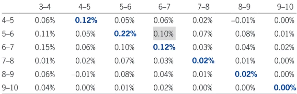
3–4 4–5 5–6 6–7 7–8 8–9 9–10

4–5 0.06% 0.12% 0.05% 0.06% 0.02% -0.01% 0.00%

5–6 0.11% 0.05% 0.22% 0.10% 0.07% 0.08% 0.01%

6–7 0.15% 0.06% 0.10% 0.12% 0.03% 0.04% 0.02%

7–8 0.01% 0.02% 0.07% 0.03% 0.02% 0.01% 0.00%

8–9 0.06% -0.01% 0.08% 0.04% 0.01% 0.02% 0.00%

9–10 0.04% 0.00% 0.01% 0.02% 0.00% 0.00% 0.00%

The error columns covariance calculations underlying matrixC_ij are shown in Table C2.

Calculations underlying Table 8

Calculation forC_ij matrix withi= 7 [for policy years 2004–2011],j= 8 and cov(e_i,e_j)=ii′Cijij= 1.91%= sum of entries is shown in Table C3. It matches the [2011, 2012] entry in Table 8.

The calculation underlying the cell [5–6, 6–7] is shown in Table C4.

R Code used to generate Table 8

‘Data file is attached with the paper’

data <- read.csv(file.choose(), header= TRUE) attach(data)

SumVCov <- matrix(nrow=10, ncol=10) for(i in 2:11)

{

for(j in 2:11)

{

CoVar <- matrix(nrow=10, ncol=10) for (k in i:11)

{

for (w in j:11)

{

CoVar[k-i+1,w-j+1]= cov(assign (paste(“K”,k,sep= “”),assign(paste(“Interval”, k,sep= “”),subset(data, Interval= = paste (“Interval_”,k,sep= “”)))[,2]),assign(paste (“W”,w,sep= “”),assign(paste(“Interva l”,w,sep=“”),subset(data, Interval= = paste(“Interval_”,w,sep= “”)))[,2]),use= “pairwise.complete.obs”)

}

}

SumVCov[i-1,j-1]= sum(CoVar,na.rm= TRUE)

} }

SumVCov