CAS: Prediction Error of the Multivariate Additive Loss Reserving Method for Dependent Lines of Business

Additive Loss Reserving Method for

Dependent Lines of Business

by Michael Merz and Mario V. Wüthrich

ABSTRACT

Often in non-life insurance, claims reserves are the largest

position on the liability side of the balance sheet.

There-fore, the prediction of adequate claims reserves for a

port-folio consisting of several run-off subportport-folios from

dependent lines of business is of great importance for

ev-ery non-life insurance company. In the present paper, we

consider the claims reserving problem in a multivariate

context–that is, we study a special case of the multivariate

additive loss reserving model proposed by Hess, Schmidt,

and Zocher (2006) and Schmidt (2006a). This model

al-lows for a simultaneous study of the individual run-off

sub-portfolios and enables the derivation of an estimator for the

conditional mean square error of prediction (MSEP) for the

predictor of the ultimate claims of the total portfolio. We

illustrate the results using the data given in Braun (2004)

and compare them to the results derived by the

multivari-ate chain-ladder methods of Braun (2004) and Merz and

Wüthrich (2008).

KEYWORDS

1. Introduction and motivation

1.1. Claims reserving

Often in non-life insurance, claims reserves are the largest position on the liability side of the balance sheet. Therefore, given the available in-formation about the past, the prediction of an ad-equate amount of claim liability assumed by the non-life insurance company, as well as the quan-tification of the uncertainties in these reserves, is a major task in actuarial practice and science [e.g., Taylor (2000); Wüthrich and Merz (2008); Casualty Actuarial Society (2001); Teugels and Sundt (2004); England and Verrall (2002)].

1.2. Multivariate claims reserving

methods and their conditional MSEP

In the present paper, we consider the claims reserving problem for a portfolio consisting of several correlated run-off subportfolios. This si-multaneous study of several individual run-off subportfolios is motivated by the following con-siderations:

² In practice it is quite natural to subdivide a non-life run-off portfolio into several corre-lated subportfolios, such that each subportfolio satisfies certain homogeneity properties (e.g., the chain-ladder assumptions or the assump-tions of the additive method).

² It addresses the problem of dependence be-tween the run-off portfolios of different lines of business (e.g., between auto liability and general liability business).

² The multivariate approach has the advantage that by observing one run-off subportfolio we can learn about the behavior of the other run-off subportfolios (e.g., subportfolios of small and large claims).

² It resolves the problem of additivity (i.e., the estimators of the ultimate claims for the whole portfolio are obtained by summation over the estimators of the ultimate claims for the indi-vidual run-off subportfolios).

However, in the case of correlated run-off subportfolios, the calculation of the conditional mean square error of prediction (MSEP) for the predictor of the ultimate claim size of the total portfolio is more sophisticated than the calcu-lation of the conditional MSEP for the predictor of the ultimate claim size of a single run-off sub-portfolio.

An alternative idea to the simultaneous study of several individual run-off subportfolios is to calculate the reserves and their uncertainties only for the total aggregated run-off portfolio. How-ever, one should pay attention to the fact that if the subportfolios satisfy, for example, the as-sumptions of the chain-ladder or the asas-sumptions of the additive method, the aggregated run-off portfolio does not in general satisfy these as-sumptions (Ajne 1994; Klemmt 2004). There-fore, in most cases it is not a promising solution to study the aggregated portfolio for the claims reserving problem of several run-off subportfo-lios.

Holmberg (1994) was probably the first one to investigate the problem of dependence between run-off portfolios of different lines of business. Later Halliwell (1997) and Quarg and Mack (2004) [see also Merz and Wüthrich (2006)] pro-posed the first bivariate models which express the dependence between the paid and incurred losses of a single run-off subportfolio.

in a univariate way. This means the estimation of the chain-ladder factors is restricted to the data of the respective individual run-off subport-folio and therefore does not take into account the correlation structure between the different run-off subportfolios. Pröhl and Schmidt (2005) and Schmidt (2006a) showed that these univariate es-timates of the chain-ladder factors are not opti-mal in terms of a classical optiopti-mality criterion in the case of correlated run-off subportfolios and therefore one should replace the univariate esti-mators with multivariate estiesti-mators of the chain-ladder factors reflecting the correlation structure. However, their study did not go beyond best es-timators; that is, they did not derive an estima-tor for the conditional MSEP for the predicestima-tor of the ultimate claim size of the total portfolio. Finally, using a multivariate chain-ladder time-series model, Merz and Wüthrich (2008) derived an estimate for the conditional MSEP, in which the chain-ladder factors are estimated in a mul-tivariate way. That is, Merz and Wüthrich (2008) studied the conditional MSEP for the multi-variate chain-ladder estimates proposed by Pröhl and Schmidt (2005) and Schmidt (2006a).

1.3. Multivariate additive loss reserving

method

The multivariate additive loss reserving meth-od proposed by Hess, Schmidt, and Zocher (2006) and Schmidt (2006a) is based on a multi-variate linear model which is suitable for cer-tain portfolios consisting of several correlated run-off subportfolios. The additive loss reserv-ing method has the followreserv-ing features:

1. It is a very simple claims reserving method which can easily be implemented in a spread-sheet.

2. Unlike the chain-ladder method, the additive loss reserving method combines past observa-tions in the upper claims development triangle with external knowledge from experts or with

a priori information (e.g., premium, number of contracts, data from similar run-off portfo-lios, and market statistics).

3. It is applied to incremental data and thus al-lows for modeling negative incremental claims in contrast to some other models such as the (overdispersed) Poisson model [cf. Wüthrich and Merz (2008)]. This makes the additive loss reserving method suitable for the use of incurred data, which often exhibits neg-ative incremental values in later development years due to earlier overestimation of case re-serves.

uncer-Figure 1. Claims development triangle numbern

tainty are especially crucial in the development of new solvency guidelines where one exactly quantifies the risk profile of the different insur-ance companies.

More precisely, we formulate a stochastic mod-el for the multivariate additive loss reserving method to derive an estimator for the conditional MSEP using the Gauss-Markov predictor pro-posed by Hess, Schmidt, and Zocher (2006) and Schmidt (2006a). Furthermore, by means of a de-tailed example, this estimator is then compared to the estimator for the conditional MSEP of the univariate predictor (i.e., if we ignore the correla-tion structure between individual subportfolios) as well as to the estimator for the conditional MSEP of the multivariate chain-ladder methods considered by Braun (2004) and Merz and Wüthrich (2008).

2. Notation and multivariate

framework

In the sequel we assume that the data for the N_¸1 run-off subportfolios consist of run-off tri-angles of observations of the same size. How-ever, the multivariate additive loss reserving method can also be applied to other shapes of data (e.g., run-off trapezoids). In these N

trian-gles the indices

n, 1·n_·N, refer to subportfolios (triangles),

i, 0·i_·I, refer to accident years (rows), and

j, 0·j_·J, refer to development years (columns).

Figure 1 shows the claims data structure for the N claims development triangles described above. The incremental claims (i.e., incremental pay-ments, change of reported claim amount, or num-ber of reported claims with reporting delayj) of run-off triangle n for accident year i and devel-opment year j are denoted by X_i(_,n_j) and cumula-tive claims (i.e., cumulacumula-tive payments, claims in-curred, or total number of reported claims) of ac-cident year iup to development yearj are given by

C_i(_,n_j)=

j

X

k=0

X_i(_,n_k): (1)

Usually, at timeI, we have observations

D(In)=fX (n)

i,j; i+j·Ig, (2)

for all run-off subportfolios n_{2 f}1,: : :,N_g. This means that at timeI (calendar year I) we have a total of observations over all subportfolios

DN I =

N

[

n=1

DI(n), (3)

and we need to predict the random variables in its complement

DIN,c=fX (n)

i,j; i·I, i+j > I, 1·n·Ng:

(4) For the derivation of the conditional MSEP for several run-off subportfolios, it is convenient to write the data of the N subportfolios in vector form. Thus, we define the N-dimensional ran-dom vectors of incremental and cumulative pay-ments by

Xi,j= (X (1) i,j,: : :,X

(N)

i,j )0 and

C_i,j= (C_i(1)_,j ,: : :,C_i(_,N_j))0

(5)

fori_{2 f}0,: : :,I_gandj_{2 f}1,: : :,J_g. Moreover, we define theN-dimensional column vector consist-ing of ones by

1= (1,: : :, 1)02RN ₍₆₎ and denote by

D(a) = 0 B B @

a₁ 0 . ..

0 a_N

1 C C

A (7)

the N_£N-diagonal matrix of the vector a= (a₁,: : :,a_N)02RN_.

3. Multivariate additive loss

reserving method

The additive loss reserving method is easy to apply. It is based on the study of individual in-cremental loss ratios. We define fori_{2 f}0,: : :,I_g andj_{2 f}1,: : :,J_gtheN-dimensional vector of in-dividual incremental loss ratios for accident year

i and development yearj by

M_i,j= (M_i(1)_,j ,: : :,M_i(_,jN))0= V¡_i 1¢X_i,j, (8) with a volume measure

Vi=

0 B B B B B B B B B @

V_i(1,1) V_i(1,2) _{¢¢¢ ¢¢¢} V_i(1,N)

V_i(2,1) V_i(2,2) _{¢¢¢ ¢¢¢} V_i(2,N) ..

. ... . .. ...

..

. ... . .. ...

V_i(N,1) V_i(N,2) _{¢¢¢ ¢¢¢} V_i(N,N) 1 C C C C C C C C C A ,

(9) which is a deterministic positive definite sym-metric N_£N-matrix. The component M_i(_,jn) of

M_i,j denotes the individual incremental loss ratio (relative to V_i) for accident year i and develop-ment year j of subportfolion.

In the univariate caseN = 1 we have

M_i,j=X_i,j=V_i, (10) whereV_i is an appropriate (deterministic) volume measure. If X_i,j denotes incremental payments and V_i is the total premium received for accident year i, then M_i,j tells how the total loss ratio is paid over time.

3.1. Multivariate additive loss reserving

model

The following multivariate additive loss reserv-ing model is a special case of the multivariate claims reserving model studied by Hess, Schmidt, and Zocher (2006) and Schmidt (2006a).

MODELASSUMPTIONS3.1 (MULTIVARIATE ADDITIVE MODEL)

² Incremental payments of different accident yearsi are independent.

² There exist N_£N-dimensional deterministic positive definite symmetric matrices V0,: : :, VI

and N-dimensional constants (j= 1,: : :,J)

mj= (m (1) j ,: : :,m

(N)

j )0 and

¾j¡1= (¾ (1) j_¡1,: : :,¾

(N) j_¡1)0

with¾(_jn_¡)₁>0 for alln= 1,: : :,N as well asN -dimensional random variables

"i,j= (" (1) i,j,: : :,"

(N)

i,j )0, (12)

such that for alli_{2 f}0,: : :,I_gandj_{2 f}1,: : :,J_g we have

X_i,j= V_i¢m_j+ V1_i=2¢D("_i,j)¢¾_j¡1: (13) Moreover, the random variables "i,j are

inde-pendent with E["_i,j] =0and

Cov("_i,j,"_i,j)

=E["i,j¢"0i,j] = 0 B B B B B B B B B @

1 ½(1,2)j_¡1 ¢¢¢ ¢¢¢ ½ (1,N)

j_¡1

½(2,1)_j¡1 1 ¢¢¢ ¢¢¢ ½(2,_j¡N₁) ..

. ... . .. ... ..

. ... . .. ...

½(jN_¡,1)1 ½ (N,2)

j_¡1 ¢¢¢ ¢¢¢ 1

1 C C C C C C C C C A

,

(14)

where ½(_jn_¡,m₁)₂(¡1, 1) forn,m_{2 f}1,: : :,N_g and n₆=m.

Clearly, in most practical applications V_i is chosen to be diagonal so as to represent a volume measure of accident year i, known a priori (e.g., premium, number of contracts, expected num-ber of claims, etc.), or an estimate from exter-nal knowledge such as experts, similar portfo-lios, or market statistics (see Example in Section 6). However, we can also take into account that the volume measure or estimate from external

knowledge for subportfolio minfluences the in-cremental payments for another subportfolio n in accident yeari by choosingV_i(n,m)₆= 0. In this case we obtain a nondiagonal matrix Vi.

In the univariate caseN= 1, the additive model satisfies

X_i,j=V_i=m_j+V_i¡1=2_¢¾_j¡1¢"_i,j, (15) with

E[X_i,j] =V_i¢m_j and

Var(X_i,j) =V_i¢¾2_j¡1: (16) Hence this model can also be interpreted as a GLM model with Gaussian variance function (i.e., V(x) = 1), volume measure V_i and disper-sion parameter ¾2_j¡1 [cf. McCullagh and Nelder (1989)].

Under Model Assumptions 3.1 we have Cov(Xi,j,Xi,j) = V

1=2

i ¢§j_¡1¢V 1=2

i , (17)

where

§_j¡1= E[D("i,j)¢¾j¡1¢¾j0_¡1¢D("i,j)]

= D(¾_j¡1)¢Cov("_i,j,"_i,j)¢D(¾_j¡1)

= 0 B B B B B B B B B B @

(¾(1)_j¡1)2 _¾(1) j¡1¾

(2) j¡1½

(1,2)

j¡1 ¢¢¢ ¢¢¢ ¾ (1) j¡1¾

(N) j¡1½

(1,N) j¡1

¾(2)_j¡1¾_j(1)_¡1½(2,1)_j¡1 (¾_j(2)_¡1)2 ¢¢¢ ¢¢¢ ¾(2)_j¡1¾_j(N_¡)₁½(2,_j¡N₁) ..

. ... ...

..

. ... ...

¾(_jN_¡)₁¾_j(1)_¡1½(_jN_¡,1)₁ ¾_j(N_¡1)¾(2)_j¡1½(_jN_¡1,2) _{¢¢¢ ¢¢¢} (¾_j(N_¡)₁)2 1 C C C C C C C C C C A

: (18)

the incremental claims of the same calender year (diagonals of the claims development triangles). However, this would contradict the assumption of independent accident years which is common to most claims reserving methods, and in fact also necessary to develop reasonable estimators from a mathematical point of view.

The Multivariate Additive Model 3.1 is a spe-cial case of the multivariate claims reserving model proposed by Hess, Schmidt, and Zocher (2006) and Schmidt (2006a), in contrast to which we assume that incremental payments X_i,j are independent (instead of only uncorrelated) and generated by the time series (13).

REMARK3.2

² The incremental claims Xi,j andXk,l are

inde-pendent for i₆=k orj₆=l.

² The N-dimensional expected incremental loss ratios (mj)1_·j_·J can be interpreted as a

multi-variate scaled expected reporting/cashflow pat-tern over the different development years.

² In (17) we use the notation §_j¡1 instead of§_j since it simplifies the comparability with the derivations and results in Merz and Wüthrich (2008).

² Since we assume that Vi is a positive

defi-nite symmetric matrix, there is a well-defined positive definite symmetric matrix V1_i=2(called square root of V_i) satisfying V_i= V1_i=2¢V1_i=2. We obtain for the conditional expectation (best estimate) E[C_{i,J j D}N

I ] of the ultimate claim

Ci,J:

PROPERTY3.3. Under Model Assumptions 3.1 we have for allI_¡J+ 1·i_·I

E[C_{i,Jj DI}N] =E[C_{i,J j}C_i,I¡i]

=C_i,I¡i+ V_i¢ J

X

j=I_¡i+1

m_j:

(19)

PROOF Using the independence of the

incre-mental claims we obtain

E[C_{i,J j D}N_I ] =C_i,I¡i+E 2 4

J

X

j=I¡i+1

X_i,j

¯ ¯ ¯ ¯ ¯D

N I

3 5

=C_i,I¡i+

J

X

j=I¡i+1

E[X_i,j]

=Ci,I_¡i+ Vi¢ J

X

j=I_¡i+1

mj

=E[C_i,J jC_i,I¡i]: (20)

This finishes the proof. Q.E.D.

This result motivates an algorithm for estimat-ing the expected ultimate claims given the obser-vationDN

I . If theN-dimensional expected

incre-mental loss ratios (m_j)_1·j·J are known, the ex-pected outstanding claims liabilities of accident yearifor theN correlated run-off triangles based on the informationDN

I are estimated by E[Ci,Jj DIN]¡Ci,I_¡i= Vi¢

J

X

j=I_¡i+1

mj: (21)

However, in most practical applications we have to estimate the ratios m_j from the data in the upper left triangle. Hess, Schmidt, and Zocher (2006) and Schmidt (2006a) propose the follow-ing multivariate estimates, for j= 1,: : :,J

ˆ

mj= ( ˆm(1)j ,: : :, ˆm (N) j )0

= 0 @

I¡j

X

i=0

V1_i=2¢§_j¡_¡1_1¢V1_i=2 1 A

¡1

¢ I_¡j

X

i=0

(V1_i=2¢§_j¡_¡1_1¢V1_i=2)¢M_i,j: (22)

The variable ˆm(_jn) denotes the estimated incre-mental loss ratio for development yearjand run-off trianglen_{2 f}1,: : :,N_gbased on the informa-tion DN

I . Note that the covariance structure

Hess, Schmidt, and Zocher (2006) and Schmidt (2006a) showed the following property, which states that the multivariate incremental loss ra-tio estimates (22) are optimal estimators of m_j

with respect to the criterion of minimal expected squared loss.

PROPERTY 3.4. Under Model Assumptions 3.1, the estimatormˆj is an unbiased estimator formj, which minimizes the expected squared loss among all N-dimensional linear combinations of the un-biased estimators(M_l,j)_0·l·I¡j form_j, i.e.,

E[(mj¡mˆj)0¢(mj¡mˆj)]

= min

Wl,j2RN£N E

2 4

0 @m_j¡

I¡j

X

l=0

Wl,j¢Ml,j

1 A

0

¢

0 @m_j¡

I_¡j

X

l=0

W_l,j¢M_l,j

1 A 3 5:

(23) PROOF See proof of Theorem 4.1 in Schmidt

(2006a). Q.E.D.

Note, in Property 3.4 we assume that the co-variance matrix §_j¡1 is known. However, if we do not have a reliable estimate for this covari-ance matrix it is often more appropriate in prac-tice to use the univariate estimators. Property 3.4 motivates the following estimator for the condi-tionally expected ultimate claim:

ESTIMATOR 3.5 (Multivariate additive estimator) The multivariate additive estimator forE[Ci,jjDIN] is fori+j_¸I given by

d

Ci,j AD

= (Cd_i(1)_,j

AD

,: : :,Cd_i(_,N_j)

AD

)0

= ˆE[C_i,jj DN

I ] =Ci,I¡i+ Vi¢ j

X

l=I_¡i+1

ˆ

m_l:

(24) This means that in the multivariate additive meth-od we predict the normalized cumulative claims V¡_i 1¢C_i,j by the sum of the last observed nor-malized cumulative claims V¡_i 1¢Ci,I_¡i and the

weighted estimated ratios ˆm_I¡i+1,: : :, ˆm_j, given the informationDN

I . From (24) we obtain for the

incremental payments X_i,j withi+j > I the pre-dictors

d

Xi,j AD

= (Xd_i(1)_,j

AD

,: : :,Xd_i(_,N_j)

AD

)0

= V_i¢mˆ_j: (25)

REMARK3.6

² In the casej=J (note that we assume I=J) we have ˆm_J =M_0,J.

² Estimator (22) is a weighted average of the observed individual normalized incremental claims M_i,j. In the case N= 1 (i.e., only one run-off subportfolio), the estimators (22) coin-cide with the univariate estimated incremental loss ratios

ˆ m_j=

I_¡j

X

i=0

V_i PI¡j

k=0Vk

¢M_i,j (26)

with deterministic weights V_i, which are used in the univariate additive loss reserving meth-od, and from Estimator 3.5 we obtain the uni-variate additive estimator

d

C_i,JAD=C_i,I¡i+

J

X

j=I¡i+1

PI¡j k=0Xk,j

PI¡j k=0Vk

¢V_i

(27) [see, for example, Schmidt (2006a; 2006b)].

² If we neglect the covariance structure between the incremental claims in the different run-off subportfolios [i.e., in (22) we set §_j¡1= I, where I denotes the identity matrix], we ob-tain the following (unbiased) estimator

ˆ

m(0)_j = 0 @

I¡j

X

i=0

Vi

1 A

¡1 ¢

I¡j

X

i=0

Vi¢Mi,j: (28)

Moreover, if the volumes Vi are diagonal

ma-trices, then the components of (28) are given by

ˆ

m(_jn)(0)=

I¡j

X

i=0

V_i(n,n) PI¡j

k=0V (n,n) k

¢M_i(_,jn): (29)

This means that in this case the components of ˆm(0)_j are given by the estimators of the uni-variate additive loss reserving method.

ˆ

m(1)_j ,: : :, ˆm(_jN) of (22) coincide with the univariate estimators (29) for the N run-off subportfolios. This means that if§₀,: : :,§_J¡2and V₀,: : :, V_I are diagonal matrices, the following estimates coin-cide: 1) the estimation for the whole portfolio based on the univariate estimators (26) for every individual run-off subportfolio, 2) the multivari-ate prediction based on the estimators (28), and 3) the multivariate prediction based on the mul-tivariate estimators (22). However, Property 3.4 shows in other cases it is more reasonable to use the multivariate estimators (22). Moreover, under Model Assumptions 3.1 it holds:

PROPERTY3.7. Under Model Assumptions 3.1 we have

a) mˆj and mˆk are independent for j6=k; b) Var( ˆmj) =

³PI¡j l=0V

1=2 l ¢§¡

1 j¡1¢V

1=2 l

´_¡1 ;

c) givenC_i,I¡i, the estimatorCd_i,JADis an unbiased estimator for E[Ci,Jj DIN] =E[Ci,J jCi,I¡i], i.e., E[Cd_i,JAD_jC_i,I¡i] =E[C_{i,Jj D}N

I ];

d) Cd_i,JAD is an unbiased estimator for E[C_i,J], i.e., E[Cd_i,JAD] =E[C_i,J].

PROOF a) Follows from the independence of the

normalized incremental claims Mi,j= V¡i 1¢Xi,j

and M_k,l= V¡_k1¢X_k,l forj₆=l. b) Using (17) we obtain

Var(Ml,j) = V¡l1¢Var(Xl,j)¢V¡l1

= V¡_l1=2¢§_j¡1¢V¡_l 1=2: (30) With the independence of the Ml,j this leads to

Var( ˆm_j) = A_j¢Var 0 @

I_¡j

X

l=0

(V1_l=2¢§_j¡_¡1_1¢V1_l=2)¢M_l,j

1 A_¢A_j

= Aj¢

2 4

I¡j

X

l=0

(V_l1=2¢§_j¡_¡1_1¢V_l1=2)¢Var(Ml,j)¢(V 1=2 l ¢§¡

1 j_¡1¢V

1=2 l )

3 5_¢Aj

= A_j¢

2 4

I_¡j

X

l=0

V1_l=2¢§_j¡_¡1_1¢V1_l=2 3 5_¢A_j

= Aj, (31)

where

Aj=

0 @

I¡j

X

l=0

V1_l=2¢§_j¡_¡1_1¢V1_l=2 1 A

¡1

: (32)

c) We have E[Cdi,J

AD

jCi,I¡i]

=C_i,I¡i+ Vi¢ J

X

l=I¡i+1

E[ ˆm_l]

=C_i,I¡i+ Vi¢ J

X

l=I¡i+1

m_l=E[C_{i,J j D}N_I ]: (33) d) Follows immediately from c). This finishes

the proof. Q.E.D.

Observe that Property 3.7 c) shows that the Estimator 3.5 is an unbiased estimator for E[C_i,Jj DN

I ]. Furthermore, this immediately

im-plies that the estimator for the aggregated ulti-mate claim of one single accident year

N

X

n=1

d C_i(_,n_J)

AD

=10¢Cdi,J AD

(34)

is, given C_i,I¡i, an unbiased estimator for PN

n=1E[C (n) i,J j DIN].

4. Conditional MSEP

In this section we consider the uncertainty in the claims reserves predicted by the estimators PN

n=1Cd (n) i,J

AD

andPI_i=1PN_n=1Cd_i(_,n_J)

AD

ob-servations DN

I . This means our goal is to derive

an estimate of the conditional MSEP for individ-ual accident years i_{2 f}1,: : :,I_gwhich is defined as

msepP nC

(n)

i,JjDNI Ã _N

X

n=1

d C_i(_,n_J)

AD! =E 2 4 Ã _N X n=1 d C_i(_,n_J)

AD ¡

N

X

n=1

C_i(_,n_J) !2¯¯

¯ ¯ ¯ ¯D N I 3 5

=10_¢E[(dC_i,JAD_¡C_i,J)_¢(Cd_i,JAD_¡C_i,J)0_{j DI}N]_¢1

(35) as well as an estimate of the conditional MSEP for aggregated accident years

msepP i,nC

(n)

i,JjDNI 0 @X

i,n

d C_i(_,n_J)

AD1 A =E 2 6 4 0 @X

i,n

d C_i(_,n_J)

AD

¡X

i,n C_i(_,n_J)

1 A

2¯¯

¯ ¯ ¯ ¯ ¯D N I 3 7 5: (36)

4.1. Conditional MSEP for single

accident years

We choose i_{2 f}1,: : :,I_g. Since the estimator PN

n=1Cd (n) i,J

AD

is known at time t=I (i.e., it is based on observations fromDN

I ), the conditional

MSEP (35) can be decoupled into conditional process variance and conditional estimation er-ror, that is

msepP nC

(n)

i,JjD N I Ã _N X n=1 d C_i(_,n_J)

AD!

= 10_¢Var(C_{i,Jj DI}N)¢1

| {z }

conditional process variance

+10¢(Cdi,J AD

¡E[Ci,J j DIN])¢(Cdi,J AD

¡E[Ci,J j DNI ])0¢1

| {z }

conditional estimation error

: (37)

The conditional process variance originates from the stochastic movement of C_i,J, whereas the conditional estimation error reflects the uncer-tainty in the estimation of the conditional expec-tation (best estimate) E[C_i,J j DN

I ]. In the sequel

we derive estimates for both the conditional pro-cess variance and the conditional estimation error forN correlated run-off triangles.

4.1.1. Conditional process variance

In this subsection we derive an estimate for the conditional process variance of a single accident year 10¢Var(C_i,Jj DN

I )¢1. We obtain the

follow-ing result:

PROPERTY4.1. (Process variance for a single

ac-cident year) Under Model Assumptions 3.1 the conditional process variance for the ultimate claim

C_i,J of accident yeari_{2 f}1,: : :,I_g is given by

10¢Var(Ci,Jj DIN)¢1

=10¢V1_i=2¢

0 @

J

X

j=I¡i+1

§_j¡1 1

A_¢V1_i=2¢1:

(38) PROOF Using the independence of the

incre-mental claim payments X_i,j we have

10_¢Var(C_{i,J j DI}N)¢1=10_¢Var 0 @

J

X

j=I¡i+1

X_i,j

1 A_¢1

=10¢

0 @

J

X

j=I_¡i+1

Var(X_i,j) 1 A_¢1

=10_¢V1_i=2¢

0 @

J

X

j=I¡i+1

§_j¡1 1

A_¢V1_i=2¢1 (39)

fori > I_¡J. This completes the proof. Q.E.D.

accident year i

10_¢Var(C_{i,jj DI}N)_¢1=10_¢(Var(C_{i,j¡1j D}N_I )

+ V1_i=2_¢§_j¡1¢V1_i=2)_¢1, (40) forj=I_¡i+ 1,: : :,J with Var(C_i,I¡ij DN

I ) =0.

4.1.2. Conditional estimation error

Now we estimate the uncertainty in the esti-mation of E[C_{i,Jj D}N

I ] by the estimator Cdi,J AD

. This means we derive an estimator for the second term on the right-hand side of (37). We estimate the conditional estimation error by its expected value

10¢E[(Cdi,J AD

¡E[Ci,Jj DIN])

¢(Cd_i,JAD_¡E[C_{i,Jj DI}N])0]¢1: (41) We obtain the following result:

PROPERTY 4.2. (Estimator of the estimation

er-ror for a single accident year) Under Model Assumptions 3.1 the estimator (41) of the

condi-tional estimation error for PN_n=1Cd_i(_,n_J)

AD

with i₂ f1,: : :,I_g is given by

10_¢E[Var(Cd_i,JAD_jC_i,I¡i)]_¢1

=10_¢V_i¢ 2 4

J

X

j=I¡i+1

ÃI¡j

X

l=0

V1_l=2_¢§_j¡_¡1_1¢V1_l=2 !¡13

5

¢V_i¢1: (42)

PROOF Using Properties 3.7 a)—b) we obtain

10_¢E[(Cd_i,JAD_¡E[C_{i,Jj DI}N])¢(Cd_i,JAD_¡E[C_{i,Jj DI}N])0]¢1

=10¢E 2 4

0 @

J

X

j=I¡i+1

Vi¢( ˆmj¡mj)

1 A_¢

0 @

J

X

j=I¡i+1

Vi¢( ˆmj¡mj)

1 A

03

5_¢1

=10¢V_i¢

0 @

J

X

j=I¡i+1

Var( ˆm_j) 1

A_¢V_i¢1 (43)

=10¢V_i¢

2 6 4

J

X

j=I_¡i+1

0 @

I_¡j

X

l=0

V1_l=2¢§_j¡_¡1_1¢V1_l=2 1 A

¡13

7

5¢V_i¢1: (44)

On the other hand, using Property 3.7 c), we have

10¢E[(Cd_i,JAD¡E[C_i,Jj DN I ]) ¢(Cd_i,JAD_¡E[C_{i,Jj D}N_I ])0]¢1

=10¢E[Var(Cdi,J AD

jCi,I_¡i)]¢1: (45)

This finishes the proof. Q.E.D.

Note, we can rewrite (42) in the recursive form

10_¢E[Var(dC_i,jAD_jC_i,I¡i)]_¢1

=10_¢E[Var(Cd_i,j¡1AD_jC_i,I¡i)]_¢1

+10_¢V_i¢ Ã_XI¡j

l=0

V1_l=2_¢§_j¡_¡1_1¢V1_l=2 !¡1

¢V_i¢1

(46)

for j=I_¡i+ 1,: : :,J with Var(Cdi,I¡i AD

jCi,I¡i)

=0.

Finally, replacing the parameters §_j¡1 in (38) and (42) by their estimates (see Section 5), we obtain the following estimator of the conditional MSEP for a single accident year:

RESULT4.3. (Conditional MSEP for a single

have the estimator for the conditional MSEP of the ultimate claim for a single accident year i₂ fI_¡J+ 1,: : :,I_g

d msepP

nC

(n)

i,JjD N I Ã _N X n=1 d C_i(_,n_J)

AD!

=10_¢V1_i=2_¢

J

X

j=I¡i+1

ˆ

§_j¡1¢V1_i=2_¢1

+10_¢V_i¢ 2 4

J

X

j=I¡i+1

Ã_I¡j X

l=0

V_l1=2_¢§ˆ_j¡_¡1_1¢V1_l=2 !¡13

5

¢V_i¢1, (47)

where the estimated covariance matrix §ˆ_j¡1 is given in (59), below.

For N= 1 formula (47) reduces to the esti-mator of the conditional MSEP for a single port-folio in the univariate additive loss reserving method

d

msepCi,JjDI(Cdi,J

AD

)

=V_i¢ J

X

j=I¡i+1

ˆ

¾2_j¡1+V_i2_¢ J

X

j=I¡i+1

ˆ ¾2_j¡1 PI¡j

l=0Vl

,

(48) where V_i is a known one-dimensional volume measure for accident yeari [cf. Mack (2002)].

4.2. Conditional MSEP for aggregated

accident years

In the following we consider the conditional MSEP for aggregated accident years. Our goal is to derive an estimate for (36). From Model As-sumptions 3.1 we know that the ultimate claims

C_i,J and C_k,J of two accident yearsi and k with 1·i < k_·Iare independent. However, since the estimatorsCd_i,JADandCd_k,JADuse the same obser-vationsDN

I for estimating the parametersmj,

dif-ferent accident years are no longer independent.

We start with the consideration of two accident years i < k

msepP

nC

(n)

i,J+ P

nC

(n)

k,JjD N I

Ã_XN

n=1

d

Ci(,nJ)

AD + N X n=1 d

Ck(n,J)

AD!

=E

2 4

Ã_XN

n=1

(dCi(,nJ)

AD

+dCk(n,J)

AD

)¡ N X

n=1

(Ci(,nJ)+C

(n)

k,J) !2¯¯

¯ ¯ ¯ ¯D N I 3 5: (49) We obtain for the conditional MSEP of the sum of two accident years the decomposition into pro-cess variance and conditional estimation error which leads to

msepP nC

(n)

i,J+ P

nC

(n)

k,JjD N I Ã _N X n=1 d C_i(_,n_J)

AD + N X n=1 d C_k(n_,J)

AD!

= msepP nC

(n)

i,JjDNI Ã _N

X

n=1

d C_i(_,n_J)

AD!

+ msepP nC

(n)

k,JjD N I Ã _N X n=1 d C_k(n_,J)

AD!

+ 2¢10_¢(Cd_i,JAD_¡E[C_{i,J j D}N_I ])

¢(Cdk,J AD

¡E[Ck,J j DNI ])0¢1: (50)

This shows that we have to derive an esti-mator for the cross product [third term on the right side of (50)], which comes from the de-pendence described above. Analogously to (41), we estimate this cross product by its expected value

10_¢E[(Cd_i,JAD_¡E[C_{i,Jj DI}N])

¢(Cdk,J AD

¡E[Ck,J j DNI ])0]¢1 (51)

and obtain the following result:

iand k with1·i < k_·I is given by 10_¢E[(Cc_i,JAD_¡E[C_{i,Jj D}N

I])¢(dCk,J

AD

¡E[C_{k,Jj D}N I])0]¢1

=10_¢Vi¢ 2 4

J X

j=I¡i+1

ÃI_¡j X

l=0

V1l=2¢§¡

1

j¡1¢V 1=2

l !¡13

5¢Vk¢1:

(52) PROOF Analogously to the proof of Property 4.2

we obtain for i < k 10_¢E[(Cc_i,JAD_¡E[C_{i,Jj D}N

I])¢(dCk,J

AD

¡E[C_{k,Jj D}N I])0]¢1

=10_¢V_i¢

" J X

j=I_¡i+1

Var( ˆm_j)

#

¢V_k¢1

=10¢Vi¢ 2 4

J X

j=I¡i+1

ÃI_¡j X

l=0

V1l=2¢§j¡_¡11¢V 1=2

l !¡13

5¢Vk¢1:

(53) Q.E.D. Putting (47) and (52) in (50) leads to the fol-lowing estimator for the conditional MSEP of the ultimate claim for aggregated accident years: RESULT 4.5. (Conditional MSEP for aggregated

accident years) Under Model Assumptions 3.1 we have the estimator for the conditional MSEP of the ultimate claim for aggregated accident years

d msepP

i P

nC

(n)

i,JjD N I Ã _I X i=1 N X n=1 d C_i(_,n_J)

AD! = I X i=1 d msepP nC

(n)

i,JjD N I Ã _N X n=1 d C_i(_,n_J)

AD!

+ 2_¢ X

1·i<k·I

10_¢V_i

¢

2 4

J

X

j=I¡i+1

ÃI¡j

X

l=0

V_l1=2_¢§ˆ_j¡_¡1_1¢V1_l=2 !¡13

5_¢V_k¢1,

(54)

where the estimated covariance matrix §ˆ_j¡1 is given in (59), below.

For N = 1, formula (54) reduces to the esti-mator of the conditional MSEP for aggregated

accident years in the univariate additive method

d msepP

iCi,JjDI Ã _I

X

i=1

d C_i,JAD

! = I X i=1 d

msepCi,JjDI(Cdi,J

AD

)

+ 2¢ X 1·i<k·I

V_i¢V_k¢ J

X

j=I¡i+1

ˆ ¾2_j¡1 PI_¡j

l=0Vl

(55) with known one-dimensional volume measureV_i for accident yeari [cf. Mack (2002)].

5. Parameter estimation

For the estimation of the claims reserves and the conditional MSEP we need estimates of theN-dimensional parameters m₁,: : :,m_J and of the N_£N-dimensional covariance parameters §₀,: : :,§_J¡1.

Estimates of the multivariate incremental loss ratios m_j are given in (22). However, estimator (22) is only an implicit estimator form_j since it depends on parameter §_j¡1, which on the other hand is estimated by means of ˆmj. Therefore,

as in the multivariate chain-ladder method [cf. Merz and Wüthrich (2008)], we propose an iter-ative estimation of these parameters. In this spirit, the “true” estimation error is slightly larger be-cause it should also involve the uncertainties in the estimate of the variance parameters. In order to obtain a feasible MSEP formula we neglect this term of uncertainty.

Estimation of m_j. As starting values for the iteration we define ˆm(0)_j by (28) for j= 1,: : :,J. Estimator ˆm(0)_j is an unbiased optimal estimator for m_j if the N run-off subportfolios are uncor-related. However, if the subportfolios are corre-lated, it is still unbiased but no longer optimal (cf. Property 3.4). From ˆm(0)_j we derive an estimate

ˆ

ˆ

m(1)_j via ˆ

m(_jk)= ( ˆm(1)(_j k),: : :, ˆm(_jN)(k))0

= 0 @

I¡j

X

l=0

V1_l=2¢( ˆ§_j(k_¡)₁)¡1¢V1_l=2 1 A

¡1

¢ I¡j

X

l=0

(V1_l=2¢( ˆ§_j(k_¡)₁)¡1¢V1_l=2)¢Ml,j

(56) for j= 1,: : :,J. This algorithm is then iterated until it has sufficiently converged.

Estimation of §_j¡1. The N_£N-dimensional covariance parameters §_j¡1 are estimated iter-atively from the data for j= 1,: : :,J. A posi-tive semidefinite estimator of the posiposi-tive definite matrix§_j¡1 is given by

ˆ

§_j¡1= 1 I_¡j¢

I¡j

X

i=0

V¡_i 1=2¢(Xi,j¡Vi¢mˆ (0) j )

¢(X_i,j¡Vi¢mˆ (0) j )0¢V

¡1=2

i (57)

for j= 1,: : :,J. If the matrices Vi are all

diago-nal, the diagonal elements of the random matrix (57) are unbiased estimators of the correspond-ing diagonal elements

(¾_j(1)_¡1)2,: : :, (¾_j(N_¡)₁)2 (58) of §_j¡1. Its nondiagonal elements slightly un-derestimate the absolute value of the correspond-ing nondiagonal elements of§_j¡1. However, this lack of unbiasedness is not too important since the random matrix (57) has to be inverted any-way and the inverse of an unbiased estimator is in general not unbiased [cf. Appendix of Merz and Wüthrich (2008)].

This leads to the following iteration for the estimator of§_j¡1:

ˆ

§_j(k_¡)₁= 1 I_¡j¢

I¡j

X

i=0

V¡_i 1=2¢(Xi,j¡Vi¢mˆ (k_¡1)

j )

¢(X_i,j¡Vi¢mˆ (k¡1) j )0¢V¡

1=2

i (59)

forj= 1,: : :,J and k_¸1.

If we have enough data (i.e., we have a run-off trapezoid withI > J), we are able to estimate iteratively the parameter §_J¡1 by (59). Other-wise, we can use the estimates 'b(_jn_¡,m₁)(k) of the elements '(_jn_¡,m₁) of §_j¡1 for j_·J_¡1 in itera-tionk_¸1 [i.e.,'b_j(n_¡,m₁)(k) is an estimate of'(_jn_¡,m₁)= ¾_j(n_¡)_1¢¾(_jm_¡)_1¢½(_jn_¡,m₁) in iteration k_¸1, cf. (18)] to derive estimates'b(_Jn_¡,m₁)(k) of the elements of§_J¡1 for all 1·n_·m_·N. For example, this can be done by extrapolating the usually exponentially decreasing series

j'b(₀n,m)(k)_j,: : :,j'b(_Jn_¡,m₂)(k)_j (60)

by one additional member 'b(_Jn_¡,m₁)(k) for 1·n_· m_·N and k_¸1. However, one needs to care-fully check that the estimate ˆ§_J(k_¡)₁ is positive def-inite. In higher dimensional cases this is often nontrivial, and in fact, many choices are not positive definite, which calls for additional ad-justments. Moreover, observe that the N_£N -dimensional estimate ˆ§_j(k_¡)₁ is singular when j¸ I_¡N+ 2, since in this case the dimension of the linear space generated by any realizations of the (I_¡j+ 1) N-dimensional random vectors

V¡_i 1=2¢(X_i,j¡V_i¢mˆ(_jk¡1)) with

i_{2 f}0,: : :,I_¡j_g (61) is at most I_¡j+ 1·I_¡(I_¡N+ 2) + 1 = N_¡1. Furthermore, the realizations of (61) may be (nearly) linearly dependent for some j < I_¡ N+ 2 which implies that the corresponding realization of the random matrix ˆ§_j(k_¡)₁ is ill-con-ditioned or even singular. Therefore, in practi-cal application it is important to verify whether the estimates ˆ§_j(k_¡)₁ are well-conditioned or not and to modify those estimates (e.g., by extrap-olation as in the example below) which are not well-conditioned.

es-Table 1. General liability run-off triangle (incremental claimsX_i(1)_,j), source Braun (2004)

General liability run-off triangle

AY/DY 0 1 2 3 4 5 6 7 8 9 10 11 12 13

0 59,966 103,186 91,360 95,012 83,741 42,513 37,882 6,649 7,669 11,061 ¡1,738 3,572 6,823 1,893

1 49,685 103,659 119,592 110,413 75,442 44,567 29,257 18,822 4,355 879 4,173 2,727 ¡776

2 51,914 118,134 149,156 105,825 78,970 40,770 14,706 17,950 10,917 2,643 10,311 1,414

3 84,937 188,246 134,135 139,970 74,450 65,401 49,165 21,136 596 24,048 2,548

4 98,921 179,408 170,201 113,161 79,641 80,364 20,414 10,324 16,204 ¡265

5 71,708 173,879 171,295 144,076 93,694 72,161 41,545 25,245 17,497

6 92,350 193,157 180,707 153,816 121,196 86,753 45,547 23,202

7 95,731 217,413 240,558 202,276 101,881 104,966 59,416

8 97,518 245,700 232,223 193,576 165,086 85,200

9 173,686 285,730 262,920 232,999 186,415

10 139,821 297,137 372,968 364,270

11 154,965 373,115 504,604

12 196,124 576,847

13 204,325

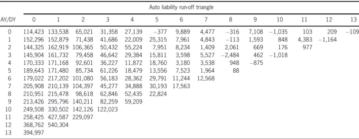
Table 2. Auto liability run-off triangle (incremental claimsX_i(2)_,j), source Braun (2004)

Auto liability run-off triangle

AY/DY 0 1 2 3 4 5 6 7 8 9 10 11 12 13

0 114,423 133,538 65,021 31,358 27,139 ¡377 9,889 4,477 ¡316 7,108 ¡1,035 103 209 ¡109

1 152,296 152,879 71,438 41,686 22,009 25,315 7,961 4,843 ¡113 1,593 848 4,383 ¡1,164

2 144,325 162,919 106,365 50,432 55,224 7,951 8,234 1,409 2,061 669 176 977

3 145,904 161,732 79,458 46,642 29,384 15,811 3,598 5,527 ¡2,484 462 ¡1,018

4 170,333 171,168 92,601 36,227 11,872 18,760 3,180 3,538 948 ¡875

5 189,643 171,480 85,734 61,226 18,479 13,556 7,523 1,964 88

6 179,022 217,202 101,080 56,183 28,362 29,791 11,244 12,568

7 205,908 210,139 104,397 45,277 34,888 30,193 17,563

8 210,951 215,478 98,618 62,846 52,435 22,824

9 213,426 295,796 140,211 82,259 59,209

10 249,508 330,502 142,126 122,023

11 258,425 427,587 229,097

12 368,762 540,304

13 394,997

timate we automatically get a well-conditioned estimate for the inverse of the covariance esti-mate. Most of these approaches rely on the con-cept of shrinkage which is quite similar to the well-known actuarial concept of credibility. For more details and other advanced methods on co-variance matrix estimation we refer to Schäfer and Strimmer (2005).

6. Example: two correlated

liability run-off subportfolios

To illustrate the methodology, we consider two correlated run-off portfolios A and B (i.e., N= 2), which contain data of general and auto lia-bility business, respectively. The data are given

in Tables 1 and 2 in incremental form. These are the data used in Braun (2004) and also in Merz and Wüthrich (2007; 2008). The assumption that there is a positive correlation between these two lines of business is justified by the fact that both run-off portfolios contain liability business; that is, certain events (e.g., bodily injury claims) may influence both run-off portfolios, and we are able to learn from the observations from one portfolio about the behavior of the other portfolio.

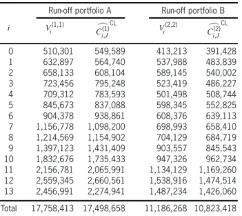
usu-Table 3. Prior estimates and chain-ladder estimates of the ultimate claims

Run-off portfolio A Run-off portfolio B

i V_i(1,1) _Cc(1)

i,J

CL

V_i(2,2) _Cc(2)

i,J

CL

0 510,301 549,589 413,213 391,428

1 632,897 564,740 537,988 483,839

2 658,133 608,104 589,145 540,002

3 723,456 795,248 523,419 486,227

4 709,312 783,593 501,498 508,744

5 845,673 837,088 598,345 552,825

6 904,378 938,861 608,376 639,113

7 1,156,778 1,098,200 698,993 658,410

8 1,214,569 1,154,902 704,129 684,719

9 1,397,123 1,431,409 903,557 845,543

10 1,832,676 1,735,433 947,326 962,734

11 2,156,781 2,065,991 1,134,129 1,169,260

12 2,559,345 2,660,561 1,538,916 1,474,514

13 2,456,991 2,274,941 1,487,234 1,426,060

Total 17,758,413 17,498,658 11,186,268 10,823,418

ally obtained from budget figures, plan values or from premium calculation parameters. Table 3 shows these a priori estimates as well as the cor-responding classical univariate chain-ladder es-timates Cd_i(1)_,J

CL

and Cd_i(2)_,J

CL

for comparison pur-poses. We see that the prior estimates and the uni-variate chain-ladder estimates are close together [for the univariate chain-ladder method see, e.g., Mack (1993) or Buchwalder, Bühlmann, Merz, and Wüthrich (2006)].

Since I=J= 13 we do not have enough data to derive an estimate of the 2£2-matrix§₁₂ us-ing estimator (59). Therefore, we use the extrap-olation

b

'₁₂(n,m)= minf('b(₁₁n,m))2=_j'b(₁₀n,m)_j,j'b(₁₀n,m)_jg (62) to derive estimates of its elements '(₁₂n,m)=¾₁₂(n)_¢ ¾₁₂(m)_¢½(₁₂n,m)forn,m= 1, 2 (note½(1,1)₁₂ =½(2,2)₁₂ = 1). Moreover, since estimator (59) would lead to an ill-conditioned matrix ˆ§₁₁, we have also esti-mated the elements of the 2£2-matrix §₁₁ by

b

'₁₁(n,m)= minf(b'₁₀(n,m))2=_j'b(₉n,m)_j,j'b(₉n,m)_jg: (63)

Table 4 shows the estimates for the parameters

m_j, ¾j and ½ (1,2)

j after three iterations k= 1, 2, 3.

We observe fast convergence of the two-dimen-sional estimates ˆm(_jk¡1), ¾b_j(k) and the one-dimen-sional estimates ˆ½(1,2)(_j k) (k= 1, 2, 3) in the sense that there are barely any changes in the estimates after three iterations. The first and second com-ponent of the estimates ˆm(0)_j and¾b(1)_j are the pa-rameter estimates used in the univariate additive method applied to the individual run-off portfo-lios A and B, respectively. Except for develop-ment years 0, 6, and 10, we observe positive esti-mates ˆ½(1,2)(_j k) for the correlation coefficients. The three negative estimates should not be overstated since they are close to zero.

Table 4. Estimatesmˆ(k_¡1)

j ,b¾

(k)

j andˆ½

(1,2)(k)

j for the parameters mj,¾jand½

(1,2)

j in the first three iterationsk= 1,2,3

A/B 0 1 2 3 4 5 6 7 8 9 10 11 12 13

ˆ

m(0)

j 0.19969 0.20638 0.17528 0.12117 0.08466 0.04852 0.02474 0.01403 0.01186 0.00606 0.00428 0.00529 0.00371 0.32897 0.16129 0.09054 0.05577 0.03166 0.01548 0.00910 0.00006 0.00349 ¡0:00050 0.00355 ¡0:00100¡0:00026

b¾(1)_j 31.58 20.03 14.42 18.92 13.64 13.91 5.79 7.15 12.21 6.09 1.84 0.56 0.17

27.74 18.19 15.17 16.00 11.74 5.17 4.70 2.05 4.96 1.35 3.00 1.35 0.61

ˆ

½(1_j:2)(1) ¡0:02644 0.84865 0.59119 0.37108 0.34004 0.31249 ¡0:10460 0.75342 0.33212 0.66573 ¡0:13915 0.14397 0.14895

ˆ

m(1)

j 0.19974 0.20640 0.17493 0.12119 0.08452 0.04844 0.02476 0.01441 0.01195 0.00614 0.00428 0.00529 0.00371 0.32899 0.16172 0.09061 0.05572 0.03170 0.01550 0.00910 0.00017 0.00354 ¡0:00051 0.00354 ¡0:00097¡0:00026

b¾(2)_j 31.58 20.03 14.42 18.92 13.64 13.91 5.79 7.16 12.21 6.09 1.84 0.56 0.17

27.74 18.20 15.17 16.00 11.74 5.17 4.70 2.05 4.96 1.35 3.00 1.35 0.61

ˆ

½(1:2)(2)

j ¡0:02654 0.84893 0.59215 0.37111 0.34034 0.31262 ¡0:10467 0.75527 0.33235 0.66612 ¡0:13921 0.14399 0.14894 ˆ

m(2)

j 0.19974 0.20640 0.17493 0.12119 0.08452 0.04844 0.02476 0.01441 0.01195 0.00614 0.00428 0.00529 0.00371 0.32899 0.16172 0.09061 0.05572 0.03170 0.01550 0.00910 0.00017 0.00354 ¡0:00051 0.00354 ¡0:00097¡0:00026

b¾(3)_j 31.58 20.03 14.42 18.92 13.64 13.91 5.79 7.16 12.21 6.09 1.84 0.56 0.17

27.74 18.20 15.17 16.00 11.74 5.17 4.70 2.05 4.96 1.35 3.00 1.35 0.61

ˆ

½(1_j:2)(3) ¡0:02654 0.84893 0.59216 0.37111 0.34034 0.31262 ¡0:10467 0.75529 0.33235 0.66612 ¡0:13921 0.14399 0.14894

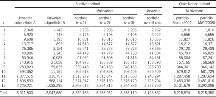
Table 5. Estimated reserves

Additive method Chain-ladder method

Multivariate Univariate Multivariate

Univariate Univariate portfolio portfolio portfolio portfolio portfolio portfolio

i subportfolio A subportfolio B (k= 1) (k= 2) (k= 3) overall calc. Braun (2004) MW (2008)

1 2,348 ¡142 2,206 2,206 2,206 2,262 1,810 1,810

2 5,923 ¡747 5,176 5,196 5,196 5,442 4,655 4,655

3 9,608 1,193 10,801 10,815 10,815 10,356 11,827 11,826

4 13,717 893 14,610 14,677 14,677 13,821 16,212 16,371

5 26,386 3,154 29,541 29,723 29,723 28,266 29,120 29,409

6 40,906 3,243 44,149 44,749 44,753 41,604 45,793 46,829

7 80,946 10,087 91,032 91,808 91,813 84,451 86,004 87,241

8 143,915 21,058 164,973 165,709 165,715 153,693 157,165 158,569

9 283,823 55,625 339,448 340,160 340,166 328,700 344,301 346,142

10 594,362 111,151 705,513 706,398 706,405 659,509 679,812 681,729

11 1,077,515 235,757 1,313,272 1,313,647 1,313,653 1,246,294 1,287,458 1,287,654

12 1,806,833 568,114 2,374,947 2,376,160 2,376,170 2,325,704 2,453,038 2,451,016

13 2,225,221 1,038,295 3,263,516 3,264,815 3,264,826 3,223,750 3,101,679 3,092,098

Total 6,311,503 2,047,680 8,359,183 8,366,062 8,366,119 8,123,852 8,218,874 8,215,350

total reserve which is about 235,300—242,300 less than the one obtained by separate calculation of the claims reserves in run-off subportfolios A and B. The last two columns show the values calculated by the multivariate chain-ladder re-serving methods proposed by Braun (2004) (i.e., chain-ladder factors are estimated in a univari-ate way) and Merz and Wüthrich (2008) (i.e.,

chain-ladder factors are estimated in a ate way), respectively. We see that the multivari-ate additive loss reserving method leads to a total reserve which is about 147,200—150,800 higher than the ones obtained by the two multivariate chain-ladder methods.

de-Table 6. Estimated conditional process standard deviations

Additive method Chain-ladder method

Multivariate Univariate Multivariate

Univariate Univariate portfolio portfolio portfolio portfolio overall portfolio portfolio

i subportfolio A subportfolio B (k= 1) (k= 2) (k= 3) calculation Braun (2004) MW (2008)

1 133 5.7% 444 ¡313:1% 483 21.9% 483 21.9% 483 21.9% 512 22.6% 1,289 71.2% 1,289 71.2%

2 471 7.9% 1,134 ¡151:8% 1,289 24.9% 1,289 24.8% 1,289 24.8% 1,275 23.4% 5,966 128.2% 5,966 128.2%

3 1,640 17.1% 2,418 202.7% 2,783 25.8% 2,783 25.7% 2,783 25.7% 2,851 27.5% 7,290 61.6% 7,290 61.6% 4 5,381 39.2% 2,552 285.9% 6,420 43.9% 6,421 43.7% 6,421 43.7% 6,196 44.8% 9,801 60.5% 9,805 59.9% 5 12,669 48.0% 4,743 150.3% 14,781 50.0% 14,782 49.7% 14,782 49.7% 14,656 51.8% 16,143 55.4% 16,149 54.9% 6 14,763 36.1% 5,043 155.5% 17,227 39.0% 17,233 38.5% 17,234 38.5% 17,020 40.9% 19,120 41.8% 19,145 40.9% 7 17,819 22.0% 6,682 66.3% 20,537 22.6% 20,544 22.4% 20,544 22.4% 20,133 23.8% 21,910 25.5% 21,937 25.1% 8 23,840 16.6% 7,989 37.9% 27,112 16.4% 27,118 16.4% 27,118 16.4% 26,640 17.3% 28,933 18.4% 28,966 18.3% 9 30,227 10.6% 14,366 25.8% 36,978 10.9% 36,985 10.9% 36,985 10.9% 37,860 11.5% 39,281 11.4% 39,322 11.4% 10 43,067 7.2% 21,419 19.3% 53,848 7.6% 53,854 7.6% 53,854 7.6% 53,978 8.2% 63,663 9.4% 63,724 9.3% 11 51,294 4.8% 28,466 12.1% 67,390 5.1% 67,404 5.1% 67,404 5.1% 69,957 5.6% 99,918 7.8% 100,004 7.8% 12 64,413 3.6% 40,112 7.1% 91,552 3.9% 91,569 3.9% 91,569 3.9% 94,860 4.1% 199,543 8.1% 199,608 8.1% 13 80,204 3.6% 51,955 5.0% 107,567 3.3% 107,580 3.3% 107,580 3.3% 110,223 3.4% 316,020 10.2% 316,020 10.2%

Total 131,444 2.1% 77,162 3.8% 174,596 2.1% 174,624 2.1% 174,624 2.1% 179,043 2.2% 396,731 4.8% 396,805 4.8%

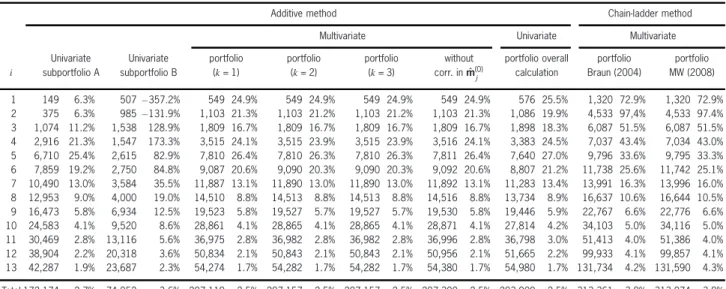
Table 7. Square roots of estimated conditional estimation errors

Additive method Chain-ladder method

Multivariate Univariate Multivariate

Univariate Univariate portfolio portfolio portfolio without portfolio overall portfolio portfolio

i subportfolio A subportfolio B (k= 1) (k= 2) (k= 3) corr. in ˆm(0)_j calculation Braun (2004) MW (2008)

1 149 6.3% 507¡357:2% 549 24.9% 549 24.9% 549 24.9% 549 24.9% 576 25.5% 1,320 72.9% 1,320 72.9%

2 375 6.3% 985¡131:9% 1,103 21.3% 1,103 21.2% 1,103 21.2% 1,103 21.3% 1,086 19.9% 4,533 97,4% 4,533 97.4%

3 1,074 11.2% 1,538 128.9% 1,809 16.7% 1,809 16.7% 1,809 16.7% 1,809 16.7% 1,898 18.3% 6,087 51.5% 6,087 51.5% 4 2,916 21.3% 1,547 173.3% 3,515 24.1% 3,515 23.9% 3,515 23.9% 3,516 24.1% 3,383 24.5% 7,037 43.4% 7,034 43.0% 5 6,710 25.4% 2,615 82.9% 7,810 26.4% 7,810 26.3% 7,810 26.3% 7,811 26.4% 7,640 27.0% 9,796 33.6% 9,795 33.3% 6 7,859 19.2% 2,750 84.8% 9,087 20.6% 9,090 20.3% 9,090 20.3% 9,092 20.6% 8,807 21.2% 11,738 25.6% 11,742 25.1% 7 10,490 13.0% 3,584 35.5% 11,887 13.1% 11,890 13.0% 11,890 13.0% 11,892 13.1% 11,283 13.4% 13,991 16.3% 13,996 16.0% 8 12,953 9.0% 4,000 19.0% 14,510 8.8% 14,513 8.8% 14,513 8.8% 14,516 8.8% 13,734 8.9% 16,637 10.6% 16,644 10.5% 9 16,473 5.8% 6,934 12.5% 19,523 5.8% 19,527 5.7% 19,527 5.7% 19,530 5.8% 19,446 5.9% 22,767 6.6% 22,776 6.6% 10 24,583 4.1% 9,520 8.6% 28,861 4.1% 28,865 4.1% 28,865 4.1% 28,871 4.1% 27,814 4.2% 34,103 5.0% 34,116 5.0% 11 30,469 2.8% 13,116 5.6% 36,975 2.8% 36,982 2.8% 36,982 2.8% 36,996 2.8% 36,798 3.0% 51,413 4.0% 51,386 4.0% 12 38,904 2.2% 20,318 3.6% 50,834 2.1% 50,843 2.1% 50,843 2.1% 50,956 2.1% 51,665 2.2% 99,933 4.1% 99,857 4.1% 13 42,287 1.9% 23,687 2.3% 54,274 1.7% 54,282 1.7% 54,282 1.7% 54,380 1.7% 54,980 1.7% 131,734 4.2% 131,590 4.3%

Total 172,174 2.7% 74,052 3.6% 207,119 2.5% 207,157 2.5% 207,157 2.5% 207,300 2.5% 203,909 2.5% 313,361 3.8% 313,074 3.8%

viations and the corresponding estimates for the coefficients of variation. The first two columns of Table 6 contain the values for the individual sub-portfolios A and B calculated by the univariate additive loss reserving method. Columns “port-folio (k= 1)” to “portfolio (k= 3)” show the es-timated conditional process standard deviations for the portfolio consisting of the two subport-folios A and B if we use the multivariate addi-tive loss reserving method (first three iterations). In particular this means that the values in col-umn k= 1 are based on the parameter estimates

ˆ

m(0)_j . The column denoted by “overall tion” shows the results for the overall calcula-tion. The last two columns show the values cal-culated by the multivariate chain-ladder reserv-ing methods proposed by Braun (2004) and Merz and Wüthrich (2008), respectively.

esti-Table 8. Estimated prediction standard errors

Additive method Chain-ladder method

Multivariate Univariate Multivariate

Univariate Univariate portfolio portfolio portfolio without portfolio overall portfolio portfolio

i subportfolio A subportfolio B (k= 1) (k= 2) (k= 3) corr. in ˆm(0)_j calculation Braun (2004) MW (2008)

1 200 8.5% 674¡475:0% 731 33.1% 731 33.1% 731 33.1% 731 33.1% 770 34.1% 1,845 101.9% 1,845 101.9%

2 602 10.2% 1,502¡201:1% 1,696 32.8% 1,697 32.6% 1,697 32.6% 1,696 32.8% 1,675 30.8% 7,493 161.0% 7,493 161.0%

3 1,961 20.4% 2,866 240.3% 3,319 30.7% 3,319 30.7% 3,319 30.7% 3,319 30.7% 3,425 33.1% 9,497 80.3% 9,497 80.3% 4 6,120 44.6% 2,984 334.3% 7,319 50.1% 7,320 49.9% 7,320 49.9% 7,320 50.1% 7,059 51.1% 12,066 74.4% 12,067 73.7% 5 14,337 54.3% 5,416 171.7% 16,717 56.6% 16,718 56.2% 16,718 56.2% 16,718 56.6% 16,528 58.5% 18,883 64.8% 18,887 64.2% 6 16,724 40.9% 5,744 177.1% 19,477 44.1% 19,484 43.5% 19,484 43.5% 19,479 44.1% 19,163 46.1% 22,435 49.0% 22,459 48.0% 7 20,677 25.5% 7,583 75.2% 23,729 26.1% 23,737 25.9% 23,737 25.9% 23,732 26.1% 23,079 27.3% 25,996 30.2% 26,022 29.8% 8 27,131 18.9% 8,935 42.4% 30,751 18.6% 30,757 18.6% 30,757 18.6% 30,753 18.6% 29,972 19.5% 33,376 21.2% 33,407 21.1% 9 34,424 12.1% 15,952 28.7% 41,815 12.3% 41,823 12.3% 41,823 12.3% 41,818 12.3% 42,562 12.9% 45,401 13.2% 45,442 13.1% 10 49,589 8.3% 23,440 21.1% 61,094 8.7% 61,102 8.6% 61,102 8.6% 61,099 8.7% 60,723 9.2% 72,222 10.6% 72,282 10.6% 11 59,660 5.5% 31,342 13.3% 76,868 5.9% 76,883 5.9% 76,883 5.9% 76,878 5.9% 79,045 6.3% 112,370 8.7% 112,434 8.7% 12 75.250 4.2% 44,965 7.9% 104,718 4.4% 104,737 4.4% 104,738 4.4% 104,777 4.4% 108,017 4.6% 223,169 9.1% 223,192 9.1% 13 90,670 4.1% 57,100 5.5% 120,484 3.7% 120,499 3.7% 120,499 3.7% 120,532 3.7% 123,174 3.8% 342,377 11.0% 342,322 11.1%

Total 216,613 3.4% 106,947 5.2% 270,891 3.2% 270,938 3.2% 270,939 3.2% 271,030 3.2% 271,358 3.3% 505,560 6.2% 505,440 6.2%

mated conditional estimation errors for the port-folio consisting of the two subportport-folios A and B if we use the multivariate additive loss reserving method. The new column “without corr. in ˆm(0)_j ” contains the estimated conditional estimation er-rors if we do not take into account correlations within the parameter estimates ˆmj and use

in-stead the estimates ˆm(0)_j . In contrast to the reserve and the conditional process standard deviation, these estimates do not coincide with the values in column “portfolio (k= 1)” since the estimator of the estimation error for a single accident year and the cross product term [i.e., right-hand side of (42) and (52)] are now given by

10_¢V_i¢ 2 4

J

X

j=I¡i+1

Ã_XI¡j

l=0

V_l !¡1

¢

Ã_XI¡j

l=0

V1_l=2_¢§_j¡1¢V1_l=2 !

¢

Ã_I¡j X

l=0

V_l !¡13

5_¢V_i¢1 (64)

and

10_¢V_i¢ 2 4

J

X

j=I¡i+1

Ã_XI¡j

l=0

V_l !¡1

¢

Ã_XI¡j

l=0

V1_l=2_¢§_j¡1¢V1_l=2 !

¢

Ã_I¡j X

l=0

V_l !¡13

5_¢V_k¢1, (65)

respectively. We see (as expected) that the esti-mation error is larger (207,300 vs. 207,157) if

we estimate the parameters on the single trian-gles. However, the difference in this example is small, which would justify working with ˆm(0)_j . The column “overall calculation” shows the es-timates for the overall calculation. The last two columns show the values calculated by the multi-variate chain-ladder reserving methods proposed by Braun (2004) and Merz and Wüthrich (2008), respectively.

Table 8 contains the estimated prediction stan-dard errors and coefficients of variation for the same set of models as above.

Table 9 contains the results for the estimated prediction standard errors assuming perfect positive correlation, no correlation, and perfect negative correlation between the corresponding claims reserves of the two run-off subportfolios A and B. These values are calculated by

d msep_C

i,JjDNI =msepd Ci(1),JjD N

I +msepd C

(2)

i,JjD N I + 2c_¢msepd 1=2

C_i(1)_,JjDN I ¢

d msep1=2