A Review of Modular Multiplication Methods ands Respective Hardware Implementation

A Review of Modular Multiplication Methods and Respective

Hardware Implementations

Nadia Nedjah

Department of Electronics Engineering and Telecommunications, Engineering Faculty, State University of Rio de Janeiro, Rio de Janeiro, Brazil

[email protected], http://www.eng.uerj.br/~nadia Luiza de Macedo Mourelle

Department of System Engineering and Computation, Engineering Faculty, State University of Rio de Janeiro, Rio de Janeiro, Brazil

[email protected], http://www.eng.uerj.br/~ldmm

Keywords: cryptography, encryption, modular multiplication, modular reduction. Received: April 18, 2005

Generally speaking, public-key cryptographic systems consist of raising elements of some group such as GF(2n), Z/NZ or elliptic curves, to large powers and reducing the result modulo some given element. Such operation is often called modular exponentiation and is performed using modular multiplications repeatedly. The practicality of a given cryptographic system depends heavily on how fast modular exponentiations are performed. Consequently, it also depends on how efficiently modular multiplications are done as these are at the base of the computation. This problem has received much attention over the years. Software as well as hardware efficient implementation were proposed. However, the results are scattered through the literature. In this paper we survey most known and recent methods for efficient modular multiplication, investigating and examining their strengths and weaknesses. For each method presented, we provide an adequate hardware implementation.

Povzetek: Podan je pregled modernih metod kriptografije.

1

Introduction

Electronic communication is growing exponentially so should be the care for information security issues [10]. Data exchanged over public computer networks must be authenticated, kept confidential and its integrity protected against alteration. In order to run successfully, electronic businesses require secure payment channels and digital valid signatures. Cryptography provides a solution to all these problems and many others [17].

One of the main objectives of cryptography consists of providing confidentiality, which is a service used to

keep secret publicly available information from all but those authorized to access it. There exist many ways to providing secrecy. They range from physical protection to mathematical solutions, which render the data unintelligible. The latter uses encryption/decryption

methods [10], [17], [30], [31].

The modular exponentiation is a common operation for scrambling and is used by several public-key cryptosystems, such Deffie and Hellman [8], [9] and the Rivest, Shamir and Adleman encryption schemes [34], as encryption/decryption method. RSA cryptosystem consists of a set of three items: a modulus M of around 1024 bits and two integers D and E called private and public keys that satisfy the property TDE≡T

mod M. Plain text T obeying 0 ≤ T < M. Messages are

encrypted using the public key as C = TE mod M and

uniquely decrypted as T = CD mod M. So the same

operation is used to perform both processes: encryption and decryption. The modulus M is chosen to be the

product of two large prime numbers, say P and Q. The

public key E is generally small and contains only few

bits set (i.e. bits = 1), so that the encryption step is relatively fast. The private key D has as many bits as the

modulus M and is chosen so that DE = 1 mod

(P−1)(Q−1). The system is secure as it is

computationally hard to discover P and Q. It has been

proved that it is impossible to break an RSA cryptosystem with a modulus of 1024-bit or more.

The modular exponentiation applies modular multiplication repeatedly. So the performance of public-key cryptosystems is primarily determined by the implementation efficiency of the modular multiplication and exponentiation. As the operands (the plaintext or the cipher text or possibly a partially ciphered text) are usually large (i.e. 1024 bits or more), and in order to improve time requirements of the encryption/decryption operations, it is essential to attempt to minimize the number of modular multiplications performed and to reduce the time required by a single modular multiplication.

Modular multiplication A×B mod M can be

interleave the multiplication and the reduction steps. There are various algorithms that implement modular multiplication. The most prominent are Karatsuba-Ofman’s [12] and Booth’s [3] methods for multiplying, Barrett’s [2], [6], [7] method for reducing, and Montgomery’s algorithms [18], and Brickell’s method [4], [37] for interleaving multiplication and reduction.

Throughout this paper, we will consider each one of the methods cited in the previous paragraph. The review will be organised as follows: First we describe, in Section 2, Karatsuba-Ofman’s and Booth’s methods for multiplying. Later, in Section 3, we present Barrett’s method for reducing an operand modulo a given modulus. Then we detail Montgomery’s algorithms for interleaving multiplication and reduction, in Section 4.

2

Efficient Multiplication Methods

The multiply-then-reduce methods consist of first computing the product then reducing it with respect to the given modulus. This method is generally preferred as there are very fast on-the-shelf multiplication algorithms as they were over studied [3], [12], [33]. The nowadays most popular multiplication methods that are suitable for hardware implementation are Karatsuba-Ofman’s method and Booth’s method.

2.1

Karatsuba-Ofman Method

Karatsuba-Ofman’s algorithm is considered one of the fastest ways to multiply long integers. Generalizations of this algorithm were shown to be even faster than Schönhage-Strassen’s FFT method [35], [36]. Karatsuba-Ofman’s algorithm is based on a divide-and-conquer strategy. A multiplication of a 2n-digit integer is reduced

to two n-digits multiplications, one (n+1)-digits

multiplication, two n-digits subtractions, two left-shift

operations, two n-digits additions and two 2n-digits

additions.

Even though this algorithm was proposed long ago and as far as we know, there is no published hardware implementation for this algorithm. In contrast with the work presented in this paper, and after an extensive paper research, we only found publications on hardware implementations of Karatsuba-Ofman’s algorithm adapted to multiplication in the Galois fields [13], [32]. Unlike in our implementation, the addition (mod 2) of two bits in these implementations delivers a single bit using a XOR gate In contrast with these, our implementation cares about the carryout bit, as it is necessary to obtaining the product. It is unnecessary to emphasize that this makes the designer face a completely different problem as explained later on.

The hardware specification is expressed using the most popular hardware description language VHDL [20]. Note that VHDL does not provide a recursive feature to implement recursive computation [1], [27], [28]. The proposed model exploits the generate feature to yield the

recursive hardware model.

This subsection is organized as follows: First, we describe the Karatsuba-Ofman’s algorithm and sketch its

complexity. Then, we adapt the algorithm so that it can be implemented efficiently. Subsequently, we propose a recursive and efficient architecture of the hardware multiplier for Karatsuba-Ofman’s algorithm. After that, we implement the proposed hardware using the Xilinx™

project manager and present some figures concerning time and space requirements of the obtained multiplier. We then compare our hardware with a Synopsis™ library

multiplier and two other multipliers that implement Booth’s multiplication algorithm.

2.1.1 Karatsuba-Ofman’s Algorithm

We now describe the details of Karatsuba-Ofman’s multiplication algorithm [12], [27], [36]. Let X and Y be

the binary representation of two long integers: X =

∑

= 1 0 2 k i i i

x and Y =

∑

We wish to compute the product XY. The operands X

and Y can be decomposed into to equal-size parts XHand

XL, YH and YL respectively, which represent the n higher

order bits and lower order bits of X and Y. Let k = 2n. If k

is odd, it can be right-padded with a zero.

X =

∑

∑

− = − = + _⎟⎟+ ⎠ ⎞ ⎜ ⎜ ⎝ ⎛ 1 0 1 0 2 2 2 n i i i n i i n i n x

x = XH 2n + XL

Y =

∑

∑

− = − = + + ⎟ ⎟ ⎠ ⎞ ⎜ ⎜ ⎝ ⎛ 1 0 1 0 2 2 2 n i i i n i i n i n y

y = YH 2n + YL

So the product P = XY can be computed as follows: P = XY

=

(

)(

)

= 22n

(

XHYH

) + 2

(

) +

Using the equation above, it needs 4 n-bits

multiplications to compute the product P. The standard

multiplication algorithm is based on that equation. So assuming that a multiplication of k-bits operands is

performed using T(k) one-bit operations, we can

formulate that T(k) =T(n) + δ k, wherein δk is a number

of one-bit operations to compute all the additions and shift operations. Considering that T(1) = 1, we find that

the standard multiplication algorithm requires:

T(k) =

(

)

( )

The computation of P can be improved by noticing

the following:

XHYL + XLYH = (XH + XL)(YH + YL) −XHYH −XLYL

The Karatsuba-Ofman’s algorithm is based on the above observation and so the 2n-bits multiplication can

be reduced to three n-bits multiplications, namely XHYH,

XLYL and (XH + XL

)(

). The Karatsuba-Ofman’s

multiplication method can then be expressed as in the algorithm in Figure 1.wherein function Size(X) returns

the number of bits of X, function High(X) returns the

higher half part of X, function Low(X) returns the lower

OneBitMultiplication(X, Y) returns XY when both X and

Y are formed by a single bit. If Size(X) is odd, then High(X) and Low(X) right-pad X with a zero before

extracting the high and the low half respectively. The algorithm above requires 3 n-bits multiplications to

compute the product P. So we can stipulate that: T(k) = 2T(n) + T(n+1)+ δ′ k ≈ 3T(n) + δ′ k

wherein δ′n is a number of one-bit operations to compute

all the additions, subtractions and shift operations. Considering that T(1) = 1, we find that the

Karatsuba-Ofman’s algorithm requires:

T(k) ≈

(

)

( )

and so is asymptotically faster than the standard multiplication algorithm.

2.1.1 Adapted Karatsuba’s Algorithm

We now modify Karatsuba-Ofman’s algorithm of Figure 1 so that the third multiplication is performed efficiently.

For this, consider the arguments of the third recursive call, which computes Product3. They have Size(X)/2+1 bits. Let Z and U be these arguments

left-padded with Size(X)/2-1 0-bits. So now Z and U have Size(X) bits. So we can write the product Product3 as

follows, wherein Size(X) = 2n, ZH and UH are the high

parts of Z and U respectively and ZLand UL are the low

parts of Z and U respectively. Note that ZH and UHmay

be equal to 0 or 1. Product3 = ZU

=

(

)(

)

= 22n

(

ZHUH

) + 2

(

) +

Depending on the value of ZH and UH, the above

expression can be obtained using one of the alternatives of Table 1.

As it is clear from Table 1, computing the third product requires one multiplication of size n and some extra

adding, shifting and multiplexing operations. So we adapt Karatsuba-Ofman’s algorithm of Figure 1 to this modification as shown in the algorithm of Figure 2.

ZH UH Product3 0 0 ZLYL

0 1 2n

ZL + ZLYL

1 0 2n

UL + ZLYL

1 1 22n _{+ 2}n

₍

UL + ZL

) +

ZLYL

Table 1: computing the third product2.1.3 Recursive Hardware Architecture

In this section, we concentrate on explaining the proposed architecture of the hardware.

The component KaratsubaOfman implements the

Algorithm KaratsubaOfman(X, Y)

If (Size(X) = 1) Then KaratsubaOfman= OneBitMultiplier(X, Y)

Else Product1 := KaratsubaOfman(High(X), High(Y));

Product2 := KaratsubaOfman(Low(X), Low(Y));

Product3 := KaratsubaOfman(High(X)+Low(X), High(Y)+Low(Y));

KaratsubaOfman := RightShift(Product1, Size(X)) +

RightShift(Product3-Product1-Product2, Size(X)/2) +

Product2;

End KaratsubaOfman.

Figure 1: Karatsuba-Ofman recursive multiplication algorithm

Algorithm AdaptedKaratsubaOfman(X, Y)

If (Size(X) = 1) Then KaratsubaOfman := OneBitMultiplier(X, Y)

Else Product1 := KaratsubaOfman(High(X), High(Y));

Product2 := KaratsubaOfman(Low(X), Low(Y));

P := KaratsubaOfman(Low(High(X)+Low(X)), Low(High(Y)+Low(Y)));

If Msb(High(X)+Low(X)) = 1 Then A := Low(High(Y)+Low(Y)) Else A := 0; If Msb(High(Y)+Low(Y)) = 1 Then B := Low(High(X)+Low(X)) Else B := 0;

Product3 := LeftShift(Msb(High(X)+Low(X))•Msb(High(X)+Low(X)), Size(X)) +

LeftShift(A + B, Size(X)/2) + P;

KaratsubaOfman = LeftShift(Product1, Size(X)) +

LeftShift(Product3-Product1-Product2, Size(X)/2) +

Product2;

End AdaptedKaratsubaOfman.

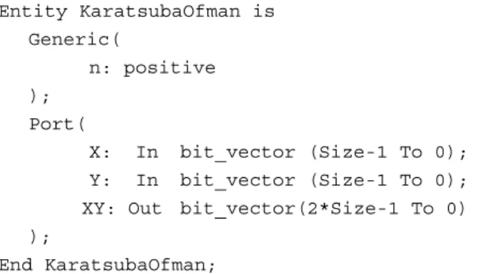
algorithm of Figure 2. Its interface is given in Figure 3. The input ports are the multiplier X and the multiplicand Y and the single output port is the product XY. It is clear

that the multiplication of 2 n-bit operands yields a

product of 2n-bits product.

The VHDL recursive specification of the component architecture is given in the concise code of Figure 4. The architecture details of the component KaratsubaOfman

are given in Figure 5.

Entity KaratsubaOfman is

Generic(

n: positive

);

Port(

X: In bit_vector (Size-1 To 0);

Y: In bit_vector (Size-1 To 0);

XY: Out bit_vector(2*Size-1 To 0)

);

End KaratsubaOfman;

Figure 3: Interface of component KaratsubaOfman The signals SXLand SYL are the two n-bits results of

the additions XH + XYand YH+ YL respectively. The two

one-bit carryout of these additions are represented in Figure 5 by CX and CY respectively.

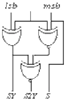
The component ShiftnAdd (in Figure 5) first

computes the sum S as SXL + SYL, SXL, SYL, or 0

depending on the values of CX and CY (see also Table 1).

Then computes Product3as depicted in Figure 6, wherein

T represents CX ×CY.

The computation implemented by component

ShiftSubnAdd (in Figure 5) i.e. the computation specified

in the last line of the Karatsuba-Ofman algorithm in Figure 1 and Figure 2 can be performed efficiently if the execution order of the operations constituting it is chosen carefully. This is shown in the architecture of Figure 7.

Figure 6: Operation performed by the ShiftnAdder2n Component ShiftSubnAdd proceeds as follows: first

computes R = Product1 + Product2; then obtains 2CR, which is the two’s complement of R; subsequently,

computes U = Product3 + 2CR; finally, as the bits of

Product1 and U must be shifted to the left 2n times and n

times respectively, the component reduces the first and last additions as well as the shift operations in the last line computation of Karatsuba-Ofman’s algorithm (see Figure 1 and Figure 2) to a unique addition that is depicted in Figure 8.

Architecture RecursiveArchitecture of KaratsubaOfman is

-- declaration part including components and temporary signals

Begin

Termination: If k = 1 Generate

TCell: OneBitMultiplier Generic Map(n) Port Map(X(0), Y(0), XY(0) );

End Generate Termination;

Recursion: If k /= 1 Generate

ADD1: Adder Generic Map(k/2) Port Map(X(k/2-1 Downto 0), X(k-1 Downto k/2), SumX );

ADD2: Adder Generic Map(k/2) Port Map(Y(k/2-1 Downto 0), Y(k-1 Downto k/2), SumY );

KO1: KaratsubaOfman Generic Map(k/2)

Port Map(X(k-1 Downto k/2),Y(k-1 Downto k/2),Product1); KO2: KaratsubaOfman Generic Map(k/2)

Port Map(X(k/2-1 Downto 0),Y(k/2-1 Downto 0),Product2);

KO3: KaratsubaOfman Generic Map(k/2)

Port Map(SumX(k/2-1 Downto 0), SumY(k/2-1 Downto 0), P);

SA: ShiftnAdder Generic Map(k)

Port Map(SumX(k/2),SY(n/2), SX(k/2-1 Downto 0), SY(k/2-1 Downto 0), P,Product3);

SSA: ShifterSubnAdder Generic Map(k) Port Map( Product1, Product2, Product3, XY );

End Generate Recursion;

End RecursiveArchitecture;

2.2

Booth’s Multiplication Method

Algorithms that formalize the operation of multiplication generally consist of two steps: one generates a partial product and the other accumulates it with the previous partial products. The most basic algorithm for multiplication is based on the add-and-shift method: the shift operation generates the partial products while the add step sums them up [3].

Figure 7: Architecture of ShiftSubnAdder2n

Figure 8: Last addition performed by ShiftSubnAdder2 The straightforward way to implement a multiplication is based on an iterative adder-accumulator for the generated partial products as depicted in Figure 9. However, this solution is quite slow as the final result is only available after n clock cycles, n is the size of the

operands.

Figure 9: Iterative multiplier

A faster version of the iterative multiplier should add several partial products at once. This could be achieved

≈ right shift

by unfolding the iterative multiplier and yielding a

combinatorial circuit that consists of several partial product generators together with several adders that operate in parallel. In this paper, we use such a parallel multiplier as described in Figure 10. Now, we detail the algorithms used to compute the partial products and to sum them up.

Figure 10: Parallel multiplier.

2.2.1 Booth’s Algorithm

Now, we concentrate on the algorithm used to compute partial products as well as reducing the corresponding number without deteriorating the space and time requirement of the multiplier.

Let X and Y be the multiplicand and multiplicator

respectively and let n and m be their respective sizes. So,

we denote X and Y as follows:

∑

∑

i Y y

x X 0 0 2 and 2 ⇒

∑

Inspired by the above notation of X, Y and that of X×Y, the add-and-shift method [2], [3] generates n partial

products: xi×Y, 0 ≤i < n. Each partial product obtained is

shifted left or right depending on whether the starting bit was the less or the most significant and added up. The number of partial products generated is bound above by the size (i.e. number of bits) of the multiplier operand. In cryptosystems, operands are quite large as they represent blocks of text (i.e. ≥ 1024 bits).

Another notation of X and Y allows to halve the

number of partial products without much increase in space requirements. Consider the following notation of X

and X×Y:

⎡ ⎤

∑

0 2 2 ~ n i i i x

X , where ~x_i=x_2×i−1+x_2×i−2×x_2×i+1

and ~x₋₁=~xn =~xn₊₁=0

⎡ ⎤

∑

The possible values of x~_iwith the respective values

of x2×i+1, x2×i, and x2×i−1 are −2 (100), −1 (101, 110), 0 (000, 111), 1 (001, 010) and 2(011). Using this recoding will generate ⎡(n+1)/2⎤−1 partial products.

Inspired by the above notation, the modified Booth algorithm [3], [12] generates the partial products x~_i×Y.

These partial products can be computed very efficiently due to the digits of the new representation x~_i. The hardware implementation will be detailed in Section 3.

In the algorithm of Figure 11, the terms 4×2n+1 _and 3_×2n+1 _{are supplied to avoid working with negative} numbers. The sum of these additional terms is congruent to zero modulo 2n+⎡(n+1)⎤ − 1_{. So, once the sum of the} partial products is obtained, the rest of this sum in the division by 2n+⎡(n+1)⎤ −1 _{is finally the result of the} multiplication X×Y.

The partial product generator is composed of kBooth recoders [3], [6]. They communicate directly with k

partial product generators as shown in Figure 12. Algorithm Booth(x2_×i-1,x2_×i,x2_×i+1,Y)

Int product := 0; Int pp[⎡(n+1)/2⎤ −1];

pp[0] := (~x₀×Y + 4×2n+1)×22×i ; For i = 0 To ⎡(n+1)/2⎤ −1 Do

pp[i] := (~x_i×Y + 3×2n+1)×22×i ; product := product + pp[i]; Return product mod 2n+⎡(n+1)⎤ − 1; End Booth

Figure 11: Multiplication algorithm

The required partial products, i.e.x~_i×Y are easy

multiple. They can be obtained by a simple shift. The negative multiples in 2’s complement form, can be obtained form the positive corresponding number using a bit by bit complement with a 1 added at the least significant bit of the partial product. The additional terms introduced in the previous section can be included into the partial product generated as three/two/one most significant bits computed as follows, whereby, ++ is the bits concatenation operation, 〈A〉 is the binary notation of

integer A, 0i is a run of i zeros and B[n:0] is the selection of

the n less significant bits of the binary representation B.

(

)

j j j

j

j s x Y s s

pp s s Y x s s s pp × × × × × × = ++ × ⊕ + ++ + ⊕ × + + = 2 2 2 2 2 2 0 0 0 0 0 0 0 0 ~ 1 ~

for 1 ≤j < k−1 and for j = k−1 = k′, we have:

Figure 12: The partial product generator architecture. The Booth selection logic circuitry used, denoted by

BRi for 0 ≤i ≤ k in Figure 12, is very simple. The cell is

described in Figure 13. The inputs are the three bits forming the Booth digit and outputs are three bits: the first one SY is set when the partial product to be

generated is Y or −Y, the second one S2Y is set when the

partial product to be generated is 2_×Y or −2×Y, the last

bit is the simply the last bit of the Booth digit given as input. It allows us to complement the bits of the partial products when a negative multiple is needed.

Figure 13: Booth recoder selection logic.

The circuitry of the partial generator denoted by PPi

Generator, is given in Figure 14.

In order to implement the adder of the generated partial products, we use a hybrid new kind of adder. It consists cascade of intercalated stages of carry save adders and delayed carry adders.

2.3

Multipliers Area/Time Requirements

The entire design was done using the Xilinx™ Project

Manager (version Build 6.00.09) [40] through the steps of the Xilinx design cycle shown in Figure 15.

Figure 14: The partial product generator.

Figure 15: Design cycle.

The design was elaborated using VHDL [20]. The

synthesis step generates an optimized netlist that is the

mapping of the gate-level design into the Xilinx format:

XNF. Then, the simulation step consists of verifying the

functionality of the elaborated design. The

implementation step consists of partitioning the design

into logic blocks, then finding a near optimal placement of each block and finally selecting the interconnect routing for a specific device family. This step generates a logic PE array file from which a bit stream can be obtained. The implementation step provides also the number of configurable logic blocks (CLBs). The

verification step allows us to verify once again the

functionality of the design and determine the response time of the design including all the delays of the physical net and padding. The programming step consists of

loading the generated bit stream into the physical device. The design was implemented into logic blocks using a specific device family, namely SPARTAN S05PC84-4.

As explained before, the Karatsuba’s multiplier reduces to an ensemble of adders. These adders are implemented using ripple-carry adders, which can be very efficiently implemented into FPGAs as the carryout signal uses dedicated interconnects in the CLB and so there is no routing delays in the data path. An n-bit

ripple-carry adder is implemented using n/2+2 CLBs and

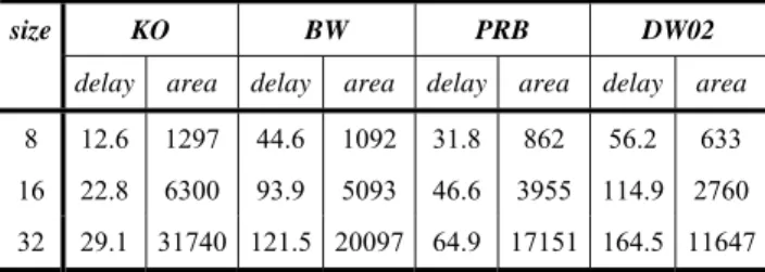
Table 2 shows the delay introduced and area required by the Karatsuba-Ofman multiplier (KO)

together with those for a hardware implementation of the Booth multiplier which uses a Wallace tree for adding up the partial products (BW), another hardware

implementation of Booth’s algorithm that uses a redundant binary Booth encoding (PRB) and the Synopsys™ library multiplier (DW02) [11]. This is given

for three different operand sizes. The delays are expressed in ns. These delays are represented graphically in Figure 16.

KO BW PRB DW02

size

delay area delay area delay area delay area

8 12.6 1297 44.6 1092 31.8 862 56.2 633

16 22.8 6300 93.9 5093 46.6 3955 114.9 2760

32 29.1 31740 121.5 20097 64.9 17151 164.5 11647

Table 2: Delays and areas for different multipliers Table 2 also shows the area required by our multiplier compared with those needed for the implementation of BW, PBR and DW02. The areas are

given in terms of total number of gates necessary for the implementation. These results are represented graphically in Figure 17.

It is clear from Figure 16 and Figure 17 that the engineered Karatsuba-Ofman multiplier works much faster than the other three multipliers. However, it

consumes more hardware area. Nevertheless, the histogram of Figure 18, which represents the area×time

factor for the four compared multipliers implementations, shows that proposed multiplier improves this product.

Figure 18: Representing area×time factor

So, our multiplier improves the area×time factor as

well as time requirement while the other three improve area at the expense of both time requirement and the

area×time factor. Moreover, we strongly think that for

larger operands, the Karatsuba-Ofman multiplier will yield very much better characteristics, i.e. time and area requirements as it is clear from Figure 16, Figure 17 and Figure 18.

3

Barrett’s Reduction Method

A modular reduction is simply the computation of the remainder of an integer division. It can be denoted by:

M M

X X M

X ×

⎥⎦ ⎥ ⎢⎣ ⎢

− =

mod

However, a division is very expensive even compared with a multiplication.

The naive sequential division algorithm successively shifts and subtracts the modulus until the remainder that is non-negative and smaller than the modulus is found. Note that after a subtraction, a negative remainder may be obtained. So in that case, the last non-negative remainder needs to be restored and so will be the expected remainder. This computation is described in the algorithm of Figure 19.

Algorithm NaiveReduction(P, M)

Int R := P;

Do R := R – M;

While R > 0;

If R ≠ 0 Then R := R + M;

Return R;

End NaiveReduction

Figure 19: Naive reduction algorithm

In the context of this paper, P is the result of a

product so it has at most 2n bits assuming that the

operands have both n bits.

The computation performed in the naïve algorithm above is very inefficient as it may require 2n

−1 subtractions, 2n _{comparisons and an extra addition.}

Instead of subtracting a single M one can subtract a

Figure 16: Representing time requirement

multiple of it at once. However, in order to yield multiples of M further computations, namely

multiplications, need be performed, except for power of two multiples, i.e. 2k

M. These are simply M left-shifted k

times, which can very cheaply implemented on hardware. This idea is described in the restoring division algorithm given in Figure 20. It attempts to subtract the biggest possible power of two multiple of M from the actual

remainder. Whenever the result of that operation is negative it restores the previous remainder and repeats the computation for all possible power of two multiples of M, i.e. 2nM, 2n−1M, …, 2M, M.

Algorithm RestoringReduction(P, M)

Int R0 := P;

Int N := LeftShift(M, n);

For i = 1 To n Do

Ri := Ri-1 – N;

If R < 0 Then Ri := Ri-1;

N := RightShift(N);

Return Ri;

End RestoringReduction

Figure 20: Restoring reduction algorithm

The computation performed in the restoring reduction algorithm requires n subtractions, n

comparisons and some 2n shifting as well as some

restoring operations. This is very much more efficient than the computation of the algorithm in Figure 19.

An alternative to the restoring reduction algorithm is the non-restoring one. The non-restoring reduction algorithm is given in Figure 21.

Algorithm NonRestoringReduction(P, M)

Int R0 := P;

Int N := LeftShift(M, n);

For i = 1 To n Do

If R > 0 Then Ri := Ri-1 – N;

Else Ri := Ri-1 + N;

N := RightShift(N);

If Ri < 0 Then Ri := Ri-1 + N;

Return Ri;

End RestoringReduction

Figure 21: Non-restoring reduction algorithm It allows negative remainder. When the remainder is non-negative it sums it up with the actual power of two multiple of M. Otherwise, it subtracts that multiple of M

from it. It keeps doing so repeatedly for all possible power of two multiples of M, i.e. 2nM, 2n−1M, …, 2M, M.

The non-restoring reduction computation requires a final restoration that adds M to the obtained remainder when

the latter is negative.

Using Barrett’s method [2], [6], we can estimate the remainder using two simple multiplications. The approximation of the quotient is calculated as follows:

⎥ ⎥ ⎥ ⎥ ⎥ ⎦ ⎥ ⎢ ⎢ ⎢ ⎢ ⎢ ⎣ ⎢ ⎥ ⎥ ⎦ ⎥ ⎢ ⎢ ⎣ ⎢ × ⎥ ⎦ ⎥ ⎢ ⎣ ⎢ = ⎥ ⎥ ⎥ ⎥ ⎥ ⎦ ⎥ ⎢ ⎢ ⎢ ⎢ ⎢ ⎣ ⎢ ⎥ ⎥ ⎦ ⎥ ⎢ ⎢ ⎣ ⎢ _× × ⎥ ⎦ ⎥ ⎢ ⎣ ⎢ = ⎥ ⎦ ⎥ ⎢ ⎣ ⎢ + × − + + − − 1 2 1 1 1 1 1 2 2 2 2 2 2 2 n n n n n n n _M X M X M X

The equation above can be calculated very efficiently as division by a power of two 2x _{are simply a truncation of}

the operand’ x-least significant digits. The term

⎣

⎦

given modulus. So, it can be pre-computed and saved in an extra register. Hence the approximation of the remainder using Barrett’s method [2], [6] is a positive integer smaller than 2×(M−1). So, one or two

subtractions of M might be required to yield the exact

remainder (see Figure 22).

4

Booth-Barrett’s Method

In this section, we outline the architecture of the multiplier, which is depicted in Figure 4. Later on in this section and for each of the main parts of this architecture, we give the detailed circuitry, i.e. that of the partial product generator, adder and reducer.

The multiplier of Figure 4 performs the modular multiplication X×Y mod M in three main steps:

1. Computing the product P = X×Y;

2. Computing the estimate quotient Q = P/M

⇒ Q ≅ P ₂n−1_×

⎣

⎦

During the first step, the modular multiplier first loads register1 and register2 with X and Y respectively;

then waits for PPG to yield the partial products and

finally waits for the ADDER to sum all of them. During

the second step, the modular multiplier loads register1, register2 and register3 with the obtained product P, the

pre-computed constant

⎣

⎦

finally waits for the ADDER to sum all of them. During

the third step, the modular multiplier first loads register1

and register2 with the obtained product Q and the

modulus M respectively; then awaits for PPG to generate

the partial products, then waits for the ADDER to provide

the sum of these partial products and finally waits for the

REDUCER to calculate the final result P−Q×M, which is

subsequently loaded in the accumulator acc.

4.1

The Montgomery Algorithm

Algorithms that formalize the operation of modular multiplication generally consist of two steps: one generates the product P = A×B and the other reduces this

product P modulo M.

The straightforward way to implement a multiplication is based on an iterative adder-accumulator for the generated partial products. However, this solution is quite slow as the final result is only available after n

clock cycles, n is the size of the operands [19].

A faster version of the iterative multiplier should add several partial products at once. This could be achieved by unfolding the iterative multiplier and yielding a

combinatorial circuit that consists of several partial product generators together with several adders that operate in parallel [15], [16].

One of the widely used algorithms for efficient modular multiplication is the Montgomery’s algorithm [18]. This algorithm computes the product of two integers modulo a third one without performing division by M. It yields the reduced product using a series of

additions

Let A, B and M be the multiplicand and multiplier

and the modulus respectively and let n be the number of

digit in their binary representation, i.e. the radix is 2. So, we denote A, B and M as follows:

2 and 2 , 2 1 0 1 0 1

0

∑

∑

∑

i B b M m

a A

The pre-conditions of the Montgomery algorithm are as follows:

The modulus M needs to be relatively prime to the radix, i.e. there exists no common divisor for M and the

radix;

The multiplicand and the multiplicator need to be smaller than M.

As we use the binary representation of the operands, then the modulus M needs to be odd to satisfy the first

pre-condition.

The Montgomery algorithm uses the least significant digit of the accumulating modular partial product to

determine the multiple of M to subtract. The usual

multiplication order is reversed by choosing multiplier digits from least to most significant and shifting down.If

R is the current modular partial product, then q is chosen

so that R+q×M is a multiple of the radix r, and this is

right-shifted by r positions, i.e. divided by r for use in the

next iteration. So, after n iterations, the result obtained is R =A×B×r−n mod M [14]. A modified version of

Montgomery algorithm is given in Figure 23.

algorithm Montgomery(A, B, M)

int R = 0;

1: for i= 0 to n-1

2: R = R + ai×B;

3: if r0 = 0 then

4: R = R div 2

5: else

6: R = (R + M) div 2;

return R;

end Montgomery.

Figure 23: Montgomery modular algorithm. In order to yield the right result, we need an extra Montgomery modular multiplication by the constant 2n

mod M. However as the main objective of the use of

Montgomery modular multiplication algorithm is to compute exponentiations, it is preferable to Montgomery pre-multiply the operands by 22n _{and Montgomery}

post-multiply the result by 1 to get rid of the 2−n _{factor. Here}

we concentrate on the implementation of the Montgomery multiplication algorithm of Figure 23.

In order to yield the right result, we need an extra Montgomery modular multiplication by the constant r2n

mod M. As we use binary representation of numbers, we

compute the final result using the algorithm of Figure 24. algorithm ModularMult(A, B, M, n)

const C := 2n mod M; int R := 0;

R := Montgomery(A, B, M);

return Montgomery(R, C, M);

end ModularMult.

Figure 24: Modular multiplication algorithm

4.2

Iterative Montgomery Architecture

Figure 25: Montgomery multiplier interface

The detailed architecture of the Montgomery modular multiplier is given in Figure 26. It uses two multiplexers, two adders, two shift registers, three registers and a controller. The latter will be described in the next section.

The first multiplexer of the proposed architecture, i.e. MUX21 passes 0 or the content of register B depending

on whether bit a0 indicates 0 or 1 respectively. The second multiplexer, i.e. MUX22 passes 0 or the content of

register M depending on whether bit r0 indicates 0 or 1 respectively. The first adder, i.e. ADDER1, delivers the

sum R + ai × B (line 2 of algorithm of Fig. 1), and the

second adder, i.e. ADDER2, yields the sum R + M (line 6

of the same algorithm). The shift register SHIFT REGISTER1provides the bit ai. In each iteration i of the

multiplier, this shift register is right-shifted once so that

a0contains ai.

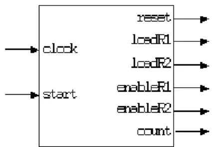
The role of the controller consists of synchronizing the shifting and loading operations of the SHIFT REGISTER1 and SHIFT REGISTER2. It also controls the number of iterations that have to be performed by the multiplier. For this end, the controller uses a simple down counter. The counter is inherent to the controller. The interface of the controller is given in Figure 27.

Figure 26: Montgomery multiplier architecture

Figure 27: Interface of the Montgomery controller In order to synchronize the work of the components of the architecture, the controller consists of a state machine, which has 6 states defined as follows:

• S0: Initialize of the state machine;

Go to S1;

• S1: Load multiplicand and modulus into

the corresponding registers;

Load multiplier into shift register1;

Go to S2; • S2: Wait for ADDER1;

Wait for ADDER2;

Load multiplier into shift register2;

Increment counter; Go to S3;

• S3: Enable shift register2;

Enable shift register1; • S4: Check the counter;

If 0 then go to S5 else go to S2; • S5: Halt;

4.3

Modular Multiplier Architecture

The modular multiplier yields the actual value of

A×B mod M. It first computes R = A×B×2−n mod M using

the Montgomery modular multiplier. Then, it computes

R × C mod M, where C = 2n mod M. The modular

multiplier interface is shown in Figure 28.

Figure 28: The modular multiplier interface The modular multiplier uses a 4-to-1 multiplexer MUX4

and a register REGISTER.

• Step 0: Multiplexer MUX4 passes 0 or B. MUX2

passes A. It yields R1 = A×B×2−n mod M. The register

denoted by REGISTER contains 0.

• Step 1: Multiplexer MUX4 passes 0 or R. MUX2

passes C. It yields R = R1×C mod M. The register denoted by REGISTER contains the result of the first

The modular multiplier architecture is given in Figure 29. In order to synchronize the actions of the components of the modular multiplier, the architecture uses a controller, which consists of a state machine of 10 states. The interface of CONTROLLER is that of Figure 30.

The modular multiplier controller does all the control that the Montgomery modular multiplier needs as described in the previous section. Furthermore, it controls the changing from step 0 to step 1, the loading of the register denoted by REGISTER. The state machine is

depicted in Figure 31.

• S0: Initialize of the state machine;

Set step to 0; Go to S1;

• S1: Load multiplicand and modulus; Load

multiplier

intoSHIFT REGISTER1;Go to S2;

Figure 29: The modular multiplier architecture

Figure 30. The interface of the multiplier controller

• S2: Wait for adder1; Wait for ADDER2;

Load partial result intoSHIFT REGISTER2;

Increment counter; Go to S3; • S3: Enable SHIFTREGISTER2;

Enable SHIFTREGISTER1; Go to S4;

• S4: Load the partial result of step 0 intoREGISTER;

Check the counter;

If 0 then go to S5 else go to S2; • S5: Load constant intoSHIFT REGISTER1;

Reset REGISTER;

Set step to 1; Go to S6;

• S6: Wait for ADDER1;Wait for ADDER2; Load partial result intoSHIFT REGISTER2; Increment counter; Go to S7;

• S7: Enable SHIFT REGISTER2;

Enable SHIFT REGISTER1; Go to S8; • S8: Check the counter;

If 0 then go to S9 else go to S6; • S9: Halt.

4.4

Simulation Results

The project of the modular multiplier described throughout this section was specified in Very High Speed Integrated Circuit Description Language - VHDL [20], and simulated using the XilinxTM Project Manager [40].

It allows the user to design and simulate the functionality

of his/her design. Moreover, it allows the synthesis of a correct design as well as its download on a specific FPGA.

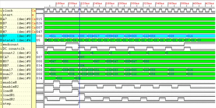
First, we functionally simulated the Montgomery modular multiplier prototype for operands A = 15, B = 26, M = 47 and so the constant C = 22x6 mod 47,

which is C = 7. The signal values are shown in

Figure 32 and Figure 33. The result is shown by signal R.

Figure 32 shows the behavior of the multiplier during the first modular multiplication (note that signal

step is not set). Figure 33 shows the results of the second

modular multiplication (note that signal step is set).

Also, we simulated the Montgomery modular multiplier prototype for bigger operand size, i.e. 16 bits. The operands are A = 120, B = 103, M = 143 and so the

constant C = 22x8 mod 143, which is C = 42. The result of

the simulation is shown in Figure 34 and Figure 35. Figure 32: The modular multiplier behavior during the first multiplication: Montgomery(15, 26, 47) = 34

As before, Figure 34 shows the behavior of the multiplier during the first modular multiplication and Figure 35 shows the results of the second modular multiplication (note that signal step is set).

4.5

Systolic Montgomery Algorithm

A modified version of Montgomery algorithm [29] is that of Figure 36. The least significant bit of R + ai×B is the

least significant bit of the sum of the least significant bits of R and B if ai is 1 and the least significant bit of R

otherwise. Furthermore, new values of R are either the

old ones summed up with ai×B or with ai×B + qi×M

depending on whether qi is 0 or 1.

algorithm ModifiedMontgomery(A, B, M) int R := 0;

1: for i := 0 to n-1

2: qi := (r0 + ai×b0) mod 2;

3: R := (R + ai×B + qi×M) div 2;

return R;

end ModifiedMontgomery.

Figure 36: Modified Montgomery algorithm Figure 34: The multiplier behavior during the first multiplication: Montgomery(120, 103, 143) = 160

Consider the expression R + ai×B + qi×M of line 2 in the

algorithm of Figure 36. It can be computed as indicated in the last column of Table 3 depending on the value of the bits ai and qi.

ai qi R + ai×B +

qi×M

1 1 R + MB

1 0 R + B

0 1 R + M

0 0 R

Table 3: Computation of R + ai×B + qi×M

A bit-wise version of the algorithm of Fig. 4, which is at the basis of our systolic implementation, is described in Figure 37. All algorithms, i.e. those of Figure 23, Figure 24 and Figure 37 are equivalent. They yield the same result. In the algorithm of Figure 37, MB represents the

result of M + B, which has at most has n + 1 bits.

4.6

Systolic Hardware Multiplier

Assuming the algorithm of Figure 37 as basis, the main processing element (PE) of the systolic architecture of the Montgomery modular multiplier computes a bit rj of

residue R. This represents the computation of line 8. The

left-border PEs of the systolic arrays perform the same computation but beside that, they have to compute bit qi

as well. This is related to the computation of line 1. The duplication of the PEs in a systolic form implements the iteration of line 0. The systolic architecture of the systolic Montgomery multiplier is shown in Figure 38.

algorithm SystolicMontgomery(A,B,M,MB) int R := 0;

bit carry := 0, x; 0: for i := 0 to n

1: qi :=

(i) 0

r _⊕ ai.b0;

2: for j := 0 to n 3: switch ai, qi

4: 1,1: x := mbi;

5: 1,0: x := bi;

6: 0,1: x := mi;

7: 0,0: x := 0;

8: r(i_j +1) := r(i)_j+1 ⊕ xi ⊕ carry;

9: carry:=r(i)_j+1.xi+

(i) 1 j

r₊ .carry+xi.carry;

return R;

end SystolicMontgomery.

Figure 37: Systolic Montgomery algorithm

The architecture of the basic PE, i.e. celli,j

1 ≤ i ≤ n−1 and 1 ≤ i ≤ n−1, is shown in Figure 39. It

implements the instructions of lines 2-9 in systolic Montgomery algorithm of Figure 37.The architecture of the right-most top-most PE, i.e. cell0,0, is given in Figure

40. Besides the computation of lines 2-9, it implements the computation indicated in line 1. However as r₀(0)is zero, the computation of q0 is reduced to a0.b0. Besides, the full-adder is not necessary as carry in signal is also 0 so r₁(0)⊕xi⊕carry and

) 0 ( 1 r .xi+

) 0 ( 1

r .carry+xi.carry

are reduced to xi and 0.

Figure 39: Basic PE architecture

Figure 40: Right-most top-most PE – cell0,0 The architecture of the rest of the PEs of the first column is shown in Figure 41. It computes q0 in the more

general case, i.e. when ₀(i)

r is not null. Moreover, the full-adder is substituted by a half-adder as the carry in signals are zero for these PEs.

The architecture of the architecture of the left border PEs, i.e. cell0,j, is given in Figure 42. As

r

full-adder is unnecessary and so it is substituted by a half-adder.

Figure 41: Right-border PEs – celli,0

Figure 42: Left-border PEs – cell0,j

The sum M+B is computed only once at the

beginning of the multiplication process. This is done by a row of full adder.

4.7

Time and Area Requirements

Consider the architecture of the systolic modular Montgomery multiplier of Figure 38. The output bit

) 1 (n+

j

r

plus an extra clock cycle, which is needed to obtain the bit mbj. So the first output bit appears after 2n + 3 clock

cycles.

Table 4 shows the performance figures obtained by the Xilinx project synthesizer for the iterative multiplier the systolic modular multiplier, wherein IM and SM stand

for iterative multiplier and systolic multiplier

respectively. The synthesis was done for VIRTEX-E [40] family.

In Table 4, we present the clock cycle time required, the area, i.e. the number of CLBs necessary as well as the

time×area product delivered by the synthesis and the

the iterative and systolic version of Montgomery multiplier.

Area

(CLBs) clock cycle time (ns) area×time operand

size

IM SM IM SM IM SM

128 89 259 46 23 4094 5957

256 124 304 102 42 12648 12767

512 209 492 199 76 41591 37392

768 335 578 207 82 69345 47396

1024 441 639 324 134 142884 85626 Table 4: Performance figures: iterative vs. systolic

The chart of Figure 43 compares the area×time product of iterative multiplier implementation vs. the systolic implementation. It shows that the latter improves the product as well as time requirement while the former improves area at the expense of both time requirement and the product.

The results show clearly that despite of requiring much more hardware area, our implementation improves substantially the time requirement and the performance factor when the operand size is bigger than 256 bits. This is almost always the case in RSA encryption/decryption systems. Nowadays, the hardware area has a very reasonable price so can be bought. However, the encryption/decryption throughput of cryptographic systems is the most fundamental characteristic and so cannot be sacrificed.

5

Further Improvements

The modular multiplication algorithm and respective hardware can be further improved if the representation of the operands is considered. The bits of the binary representation can be grouped to increase the representation base. For instance, if the bits are grouped into pairs or triples, the base will be 4 or 8 respectively. Although other bases are possible, usually a power of 2 is preferred to make conversion to and from binary easy. Increasing the base reduces the number of digits in the operand and so reduces the number of clock cycles required to complete a modular multiplication. Another improvement consists of using the so-called redundant representation of the operand together with the Montgomery algorithm. This avoids the unbounded propagation of carries.

Figure 43: The area×time factor for iterative vs. systolic

6

Discussion

As stated in the introduction, the methods used to compute modular products fall in two categories: (i)

those that first compute the product then reduced product, and (ii) those that compute the modular product

directly.

The advantage of the first category method is that one can use any on-the-shelf method for multiplication and reduction. However, the only such methods that are efficient consist of those presented here, i.e. Karatsuba-Ofman’s and Booth’s methods for multiplication and Barrett’s method for reduction. As far as the authors are concerned, these methods are the only ones appropriate for hardware implementation. Another disadvantage of using the multiply-then-reduce method is that the product is generally large and thus requires a great deal of space to store it for further use by the reduction step.

In contrast, the methods that interleave multiplication and reduction steps to produce the modular product do not have to store the product. However, also as far as the authors are concerned, only Montgomery’s method that yields the modular product in such a way. Hardware implementation of Montgomery’s algorithm always require very much less area than the implementations of the first category methods. Furthermore, these implementations are always very much slower than the implementations of Montgomery method.

7

Conclusions

In this paper we surveyed most known and recent methods for efficient modular multiplication. For each method presented, we provide an adequate hardware implementation.

We explained that the modular multiplication A×B

mod M can be performed in two different ways:

Throughout this paper, we considered each one of the methods cited previously. The review was organized as follows: First we described the Karatsuba-Ofman’s and Booth’s methods for multiplying. Subsequently, we presented Barrett’s method for reducing an operand

modulo a given modulus. For each method, we detailed

the hardware architecture and then compared the respective hardware with respect to area and response time requirements. The implementation of the modular multiplication using Karatsuba-Ofman’s method for multiplying and Barrett’s method for reducing the obtained result presents a shorter signal propagation delay than using Booth’s method together with Barrett’s method, without much increase in hardware area requirements.

After that, we detailed the Montgomery’s algorithm for interleaving multiplication and reduction. For the method, we presented two hardware implementations: one iterative and the other systolic. The systolic implementation is much better that the sequential one but requires more hardware area.

Subsequently, we reviewed some techniques that should allow further improvement to the implementation of the modular multiplication with long operand.

8

Acknowledgments

We are grateful to the reviewers and the editor that contributed to the great improvement of the original version of this paper with their valuable comments and suggestions. We also are thankful to FAPERJ (Fundação de Amparo à Pesquisa do Estado do Rio de Janeiro, http://www.faperj.br) and CNPq (Conselho Nacional de Desenvolvimento Científico e Tecnológico, http://www.cnpq.br) for their continuous financial support.

9

References

[1] Ashenden, P.J., Recursive and Repetitive Hardware Models in VHDL, Joint Technical Report, TR

160/12/93/ECE, University of Cincinnati, and TR 93-19, University of Adelaide, 1993.

[2] Barrett, P., Implementating the Rivest, Shamir and Aldham public-key encryption algorithm on standard digital signal processor, Proceedings of

CRYPTO'86, Lecture Notes in Computer Science 263:311-323, Springer-Verlag, 1986.

[3] Booth, A., A signed binary multiplication technique, Quarterly Journal of Mechanics and

Applied Mathematics, pp. 236-240, 1951.

[4] Brickell, E. F., A survey of hardware implementation of RSA, In G. Brassard, ed.,

Advances in Cryptology, Proceedings of CRYPTO'98, Lecture Notes in Computer Science 435:368-370, Springer-Verlag, 1989.

[5] S. E. Eldridge and C. D. Walter, Hardware implementation of Montgomery’s modular multiplication algorithm, IEEE Transactions on

Computers, 42(6):619-624, 1993.

[6] Bewick, G.W., Fast multiplication algorithms and implementation, Ph. D. Thesis, Department of

Electrical Engineering, Stanford University, United States of America, 1994.

[7] Dhem, J.F., Design of an efficient public-key cryptographic library for RISC-based smart cards,

Ph.D. Thesis, Faculty of Applied Science, Catholic University of Louvain, May 1998.

[8] W. Diffie and M.E. Hellman, New directions in cryptography, IEEE Transactions on Information

Theory, vol. 22, pp. 644-654, 1976.

[9] ElGamal, T., A public-key cryptosystems and signature scheme based on discrete logarithms,

IEEE Transactions on Information Theory, 31(4):469-472, 1985.

[10] Gutmann P., Cryptographic Security Architecture: Design and Verifcation, Springer-Verlag, 2004. [11] Kim, J.H., Ryu, J. H., A high speed and low power

VLSI multiplier using a redundant binary Booth encoding, Proc. of 6th Korean Semiconductor

Conference, PA-30, 1999.

[12] Knuth, D.E., The art of computer programming:

seminumerical algorithms, vol 2, 2nd Edition, Addison-Wesley, Reading, Mass., 1981.

[13] Jung, M., Madlener, F., Ernst, M. and Huss, S.A., A reconfigurable coprocessor for finite field multiplication in GF(2n), Proc. of IEEE Workshop

on Heterogeneous Reconfigurable systems on Chip, Hamburg, Germany, 2002.

[14] Koç, Ç.K., High speed RSA implementation,

Technical report, RSA Laboratories, RSA Data Security Inc. CA, version 2, 1994.

[15] Lim, C.H., Hwang, H.S. and Lee, P.J., Fast modular reduction with precomputation, In

Proceedings of Korea-Japan Joint Workshop on Information Security and Cryptology, Lecture Notes in Computer Science, 488:323-334, 1991. [16] MacSorley, O., High-speed arithmetic in binary

computers, Proceedings of the IRE, pp. 67-91,

1961.

[17] Menezes, A. van Oorschot, P. and Vanstone, S.,

Handbook of Applied Cryptography, CRC Press,

1996.

[18] Montgomery, P.L., Modular Multiplication without trial division, Mathematics of Computation,

44: 519-521, 1985.

[19] Mourelle, L.M. and Nedjah, N., Compact iterative hardware simulation model for Montgomery’s algorithm of modular multiplication, Proceedings

of ACS/IEEE International Conference on Computer Systems and Applications, Tunis, Tunisia, July 2003.

[20] Navabi, Z., VHDL - Analysis and modeling of digital systems, McGraw Hill, Second Edition,

1998.

[21] Nedjah, N. and Mourelle, L.M., Yet another implementation of modular multiplication,

[22] Nedjah, N. and Mourelle, L.M., Simulation model for hardware implementation of modular multiplication, In: Mathematics nad Simulation with Biological, Economical and Musicoacoustical Applications, C.E. D’Attellis, V.V. Kluev, N.E. Mastorakis Eds. WSEAS Press, 2001, pp. 113-118. [23] Nedjah, N. and Mourelle, L.M., Reduced hardware

architecture for the Montgomery modular multiplication, WSEAS Transactions on Systems,

1(1):63-67.

[24] Nedjah, N. and Mourelle, L.M., Two Hardware implementations for the Montgomery modular multiplication: sequential versus parallel,

Proceedings of the 15th_{. Symposium Integrated} Circuits and Systems Design, Porto Alegre, Brazil, IEEE Computer Society Press, pp. 3-8, 2002 [25] Nedjah, N. and Mourelle, L.M., Reconfigurable

hardware implementation of Montgomery modular multiplication and parallel binary exponentiation,

Proceedings of the EuroMicro Symposium on Digital System Design − Architectures, Methods and Tools, Dortmund, Germany, IEEE Computer Society Press, pp. 226-235, 2002

[26] Nedjah, N. and Mourelle, L.M., Efficienthardware implementation of modular multiplication and exponentiation for public-key cryptography,

Proceedings of the 5th_{. International Conference on} High Performance Computing for Computational Science, Porto, Portugal, Lecture Notes in Computer Science, 2565:451-463, Springer-Verlag, 2002

[27] Nedjah, N. and Mourelle, L.M., Hardware simulation model suitable for recursive computations: Karatsuba-Ofman’s multiplication algorithm, Proceedings of ACS/IEEE International

Conference on Computer Systems and Applications, Tunis, Tunisia, July 2003.

[28] Nedjah, N. and Mourelle, L.M., A Reconfigurable recursive and efficient hardware for Karatsuba-Ofman’s multiplication algorithm, Proceedings of

IEEE International Conference on Control and Applications, Istambul, Turkey, June 2003, IEEE System Control Society Press.

[29] Nedjah, N. and Mourelle, L.M. (Eds.), Embedded Cryptographic Hardware: Methodologies and Applications, Nova Science Publishers, Hauppauge, NY, USA, 2004.

[30] Nedjah, N. and Mourelle, L.M. (Eds.), Embedded Cryptographic Hardware: Design and Security, Nova Science Publishers, Hauppauge, NY, USA, 2005.

[31] Nedjah, N. and Mourelle, L.M. (Eds.), New Trends on Embedded Cryptographic Hardware, Nova Science Publishers, Hauppauge, NY, USA (to appear).

[32] Paar, C., A new architecture for a parallel finite field multiplier with low complexity based on composite fields, IEEE Transactions on Computers,

45(7):856-861, 1996.

[33] Rabaey, J., Digital integrated circuits: A design perspective, Prentice-Hall, 1995.

[34] Rivest, R., Shamir, A. and Adleman, L., A method for obtaining digital signature and public-key cryptosystems, Communications of the ACM,

21:120-126, 1978.

[35] Shindler, V., High-speed RSA hardware based on low-power piplined logic, Ph. D. Thesis, Institut für

Angewandte Informations-verarbeitung und Kommunikationstechnologie, Technishe Universität Graz, January 1997.

[36] Zuras, D., On squaring and multiplying large integers, In Proceedings of International

Symposium on Computer Arithmetic, IEEE Computer Society Press, pp. 260-271, 1993.

[37] Walter, C.D., A verification of Brickell’s fast modular multiplication algorithm, International

Journal of Computer Mathematics, 33:153:169, 1990.

[38] Walter, C.D., Systolic modular multiplication, IEEE

Transactions on Computers, 42(3):376-378, 1993. [39] Walter, C. D., Systolic modular multiplication,

IEEE Transactions on Computers, 42(3):376-378, 1993.

[40] Xilinx, Inc. Foundation Series Software,