Meenal Jain and Gagandeep Kaur
Department of Computer Science and Information Technology, Jaypee Institute of Information Technology, Noida, India
A Study of Feature Reduction
Techniques and Classification for
Network Anomaly Detection
Due to the launch of new applications the behavior of Internet traffic is changing. Hackers are always looking for sophisticated tools to launch attacks and damage the services. Researchers have been working on intrusion detection techniques involving machine learning algorithms for supervised and unsupervised detection of these attacks. However, with newly found attacks these techniques need to be refined. Handling data with large number of attributes adds to the prob-lem. Therefore, dimensionality based feature reduc-tion of the data is required. In this work three reducreduc-tion techniques, namely, Principal Component Analysis (PCA), Artificial Neural Network (ANN), and Non-linear Principal Component Analysis (NLPCA) have been studied and analyzed. Secondly, performance of four classifiers, namely, Decision Tree (DT), Support Vector Machine (SVM), K Nearest Neighbor (KNN) and Naïve Bayes (NB) has been studied for the actual and reduced datasets. In addition, novel performance measurement metrics, Classification Difference Mea-sure (CDM), Specificity Difference MeaMea-sure (SPDM), Sensitivity Difference Measure (SNDM), and F1 Dif-ference Measure (F1DM) have been defined and used to compare the outcomes on actual and reduced data-sets. Comparisons have been done using new Coburg Intrusion Detection Data Set (CIDDS-2017) dataset as well widely referred NSL-KDD dataset. Successful results were achieved for Decision Tree with 99.0 per-cent and 99.8 perper-cent accuracy on CIDDS and NSL-KDD datasets respectively.
ACM CCS (2012) Classification: Security and privacy
→ Intrusion/anomaly detection and malware mitiga-tion → Intrusion detection systems → Artificial im-mune systems
Information systems → Information systems applica-tions → Data mining → Clustering
Networks → Network performance evaluation →
Network performance analysis
Keywords: intrusion detection, dimensionality, reduc-tion, principal component analysis, nonlinear principal component analysis, artificial neural network, CIDDS, NSL-KDD
1. Introduction
pro-performed best with regard to processing time, achieving 0.02 sec and 0.39 sec, respectively. S. Mallissery, S. Kolekar and R. Ganiga in [15] have applied the PCA technique for feature re-duction. The classifiers used in this paper were Classification and Regression Tree, NB, SVM, ID3, and J48. The analysis was performed on NSL-KDD dataset, with and without dimension reduction technique. The results showed that af-ter reduction the original dataset was reduced to approximately 56.09 percent. They also showed that SVM gave better accuracy of 99.8 percent after reduction. For anomaly detection, a hybrid machine learning algorithm was proposed by A.S.A. Aziz, A.E. Hassanien, S. Hanaf et al. in [16]. In the first step, 22 attributes were select-ed using PCA. For producing detectors, Genetic Algorithm was applied in the next step, which can differentiate between attack and normal be-haviour. In the last step, various classifiers were used. The results showed that the NB classifier achieved better detection accuracy for two types of attacks, namely, U2R and R2L. The Decision Tree classifier achieved the highest accuracy of 82 percent and 65 percent for DOS and Probe attacks respectively. PCA is an effective method to reduce dimensionality of data by providing a linear transformation of high dimension to low dimensional feature space as discussed by Cu-reton and D'Agostino in [17]. Because the time complexity of PCA was high and it also failed in nonlinear mapping, an Improved Principal Com-ponent Analysis (IPCA) method was proposed for feature reduction by B. Zhang, Liu, Jia et al.
in [18]. They differentiated the proposed meth-od with traditional PCA and showed that IPCA, along with Gaussian Naïve Bayes algorithm for classification, achieved better detection rate of 91.06 percent. Also, time was reduced by 60 percent in comparison to Naïve Bayes Classifi-er. A. Jahanbani and H. Karimi in [19] proposed a new classifying system for anomaly detection, named Principal Component Analysis Neural Network (PCANN). The KDD dataset was used for analysis and testing. The results showed that in comparison with other approaches, the pro-posed approach had either the same or higher detection and false positive rate of 99.59 percent and 0.40 percent respectively. Z. Elkhadir, K. Chougdali, and B. Mohammed in [20] applied two feature reduction techniques, namely PCA and Kernel PCA (KPCA), and compared their performances. After extracting the features,
2. Literature Survey
J. P. Nziga in [12] has presented dimensional-ity reduction techniques and performed Naïve Bayes and J48 based classifications. The author has used PCA and Multidimensional Scaling for linear and nonlinear dimensionality reduc-tion and reduced the data set to four and twelve dimensions respectively. The dataset used was KDD dataset [13]. Results showed that the Naïve Bayes with twelve dimensions reduced the orig-inal dataset to 95.11 percent and J48 with four dimensions reduced dataset to 99.87 percent. K. K. Vasan and B. Surendiran in [14] focused on the efficacy of PCA for anomaly detection and extracted ten Principal Components (PCs) for classification. Two real-time intrusion detection datasets, namely, UNB ISCX and KDD were used. Reduction Ratio (RR) was studied to anal-yse the importance of PCA in detecting anoma-lies. It showed that the RR of PCA for KDD and UNB ISCX dataset was 0.24 and 0.36, respec-tively. Results showed that the classification accuracies using Random Forest (RF) and C4.5 after applying reduced dimensions on both data-sets were approximately the same as those ob-tained using original features, 98.8 percent and 99.7 percent respectively. I. S. Thaseen and C. A. Kumar in [8] have presented two-step PCA feature reduction algorithm. In the first step the variance of every attribute was calculated to find optimal principal components. Ten components with the highest variance were selected and were used in the second step as an input vector for classifier SVM to perform anomaly detection. KDD dataset was used for experiments. It was divided in two separate datasets, namely, D1 and D2. The test results showed that minimum False Positive Rates (FPR) of 0.15 percent and 0.30 percent, respectively, were achieved. F. Rahat and S. N. Ahsan in [9] have proposed a structure using two sampling methods: stratified remove folds and resample. In addition, the authors have proposed five different feature reduction tech-niques, namely, PCA, Info Gain, Gain Ratio, Chi Square and Filtered Attribute. Five different classifiers were used for classifying performance of the intrusion detection in data set, namely, J48, Naive Bayes, AdaBoost, Bagging, and Nearest Neighbour. It showed that Gain Ratio produced an optimal subset of features. Analysis was per-formed on the KDD dataset. Results showed that KNN and J48 machine learning algorithms tect the network by identifying not only the
ex-isting ones but also to successfully identify new types of attacks. Intrusion Detection Techniques (IDTs) [2] are used to detect both known and un-known types of threats. IDTs have been divided into two types, namely, (1) Signature based IDTs (SbIDTs) [3] and Anomaly based IDTs (AbIDTs) [4-6]. Pre-identified signatures for normal and attack traffic in SbIDTs are used to detect attack patterns. In AbIDTs, intrusions are identified by making a profile of normal network activity while patterns deviating from normal behaviour are considered as anomalous and later studied for presence or absence of an attack. SbIDTs de-tect already known attack patterns only and fail to identify unknown or new attacks.
Various techniques like signal processing, sta-tistical analysis, machine learning based ap-proaches, etc. have been studied and used by researchers for tackling the menace of network based attacks. In recent times, Machine Learn-ing Techniques (MLTs) have gained popularity [7]. MLTs find widespread use and are popular because of their capabilities to automatically de-tect attack patterns, identify hidden anomalies, maintain high detection accuracy with low false positive rate, and work on large data sets. Pop-ular MLTs used for classifying network traffic are Support Vector Machine (SVM) [8], Deci-sion Tree (DT), K Nearest Neighbours (KNN), Naïve Bayes (NB) [9] and so on. However, an adverse aspect of employing these classification algorithms for anomaly detection applications is their high complexity with respect to space and time, essentially due to the high dimension space in which these algorithms work. Besides, the number of input parameters required for training of these classifiers has also increased. Moreover, the rate of incoming and outgoing network traffic has also increased exponentially, thus leading to the need for studying large data sets. Therefore, study of feature reduction is required to reduce the size of the data sets in order to ensure fast and accurate application of machine learning algorithms [10]. Furthermore, traditional intru-sion detection techniques have been confined to datasets having linear data only. It has been re-alised that present nature of network traffic data is non-linear and that appropriate techniques of machine learning should be explored.
Varied numbers of datasets related to computer networks traffic are available in the public
do-main. KDD Dataset which was later converted to NSL-KDD Dataset, after removing its incon-sistencies for applying MLTs, has been a data-set widely studied by the researchers' commu-nity. However, it is quite old for studying new varieties of attacks that have cropped up on the Internet. Henceforth, a study of newer datasets is needed. Some of the new benchmark public datasets are CAIDA Dataset, LBNL Dataset, CIDDS Dataset, UNSW, CICIDS2017 Dataset, UNB-ISCX, etc. These are available in the net-work anomaly detection domain [11]. We have worked on CIDDS Dataset due to two main fac-tors: firstly, it covers some of the new attack types and, secondly, due to its size.
In this paper, we have worked on three feature reduction methods, namely, Principal Compo-nent Analysis (PCA), Artificial Neural Net-work (ANN) and Nonlinear Principal Compo-nent Analysis (NLPCA). Four classifiers have been applied, namely, Support Vector Machine (SVM), Decision Tree (DT), Naïve Bayes (NB), and K Nearest Neighbours (KNN) to verify the effect of the new reduced sets of features on the detection accuracy and false positive rate. In do-ing so, the main contributions of our work are:
● reduction of the dimensionality of the net-work traffic of recent dataset so as to lessen computational time and space complexity;
● generation of new dataset from dimension-ally reduced data while maintaining the relevant features required for successful identification of new anomalies;
● applying ML Classifiers to measure per-formance evaluation metrics;
● maintaining or increasing detection accu-racy and reducing false positive rate;
● define novel performance measures, Clas-sification Difference Measure (CDM), Specificity Difference Measure (SPDM), Sensitivity Difference Measure (SNDM), F1 Difference Measure (F1DM) and Com-bined Performance Measure (CPM) to analyse the outputs.
performed best with regard to processing time, achieving 0.02 sec and 0.39 sec, respectively. S. Mallissery, S. Kolekar and R. Ganiga in [15] have applied the PCA technique for feature re-duction. The classifiers used in this paper were Classification and Regression Tree, NB, SVM, ID3, and J48. The analysis was performed on NSL-KDD dataset, with and without dimension reduction technique. The results showed that af-ter reduction the original dataset was reduced to approximately 56.09 percent. They also showed that SVM gave better accuracy of 99.8 percent after reduction. For anomaly detection, a hybrid machine learning algorithm was proposed by A.S.A. Aziz, A.E. Hassanien, S. Hanaf et al. in [16]. In the first step, 22 attributes were select-ed using PCA. For producing detectors, Genetic Algorithm was applied in the next step, which can differentiate between attack and normal be-haviour. In the last step, various classifiers were used. The results showed that the NB classifier achieved better detection accuracy for two types of attacks, namely, U2R and R2L. The Decision Tree classifier achieved the highest accuracy of 82 percent and 65 percent for DOS and Probe attacks respectively. PCA is an effective method to reduce dimensionality of data by providing a linear transformation of high dimension to low dimensional feature space as discussed by Cu-reton and D'Agostino in [17]. Because the time complexity of PCA was high and it also failed in nonlinear mapping, an Improved Principal Com-ponent Analysis (IPCA) method was proposed for feature reduction by B. Zhang, Liu, Jia et al.
in [18]. They differentiated the proposed meth-od with traditional PCA and showed that IPCA, along with Gaussian Naïve Bayes algorithm for classification, achieved better detection rate of 91.06 percent. Also, time was reduced by 60 percent in comparison to Naïve Bayes Classifi-er. A. Jahanbani and H. Karimi in [19] proposed a new classifying system for anomaly detection, named Principal Component Analysis Neural Network (PCANN). The KDD dataset was used for analysis and testing. The results showed that in comparison with other approaches, the pro-posed approach had either the same or higher detection and false positive rate of 99.59 percent and 0.40 percent respectively. Z. Elkhadir, K. Chougdali, and B. Mohammed in [20] applied two feature reduction techniques, namely PCA and Kernel PCA (KPCA), and compared their performances. After extracting the features,
2. Literature Survey
J. P. Nziga in [12] has presented dimensional-ity reduction techniques and performed Naïve Bayes and J48 based classifications. The author has used PCA and Multidimensional Scaling for linear and nonlinear dimensionality reduc-tion and reduced the data set to four and twelve dimensions respectively. The dataset used was KDD dataset [13]. Results showed that the Naïve Bayes with twelve dimensions reduced the orig-inal dataset to 95.11 percent and J48 with four dimensions reduced dataset to 99.87 percent. K. K. Vasan and B. Surendiran in [14] focused on the efficacy of PCA for anomaly detection and extracted ten Principal Components (PCs) for classification. Two real-time intrusion detection datasets, namely, UNB ISCX and KDD were used. Reduction Ratio (RR) was studied to anal-yse the importance of PCA in detecting anoma-lies. It showed that the RR of PCA for KDD and UNB ISCX dataset was 0.24 and 0.36, respec-tively. Results showed that the classification accuracies using Random Forest (RF) and C4.5 after applying reduced dimensions on both data-sets were approximately the same as those ob-tained using original features, 98.8 percent and 99.7 percent respectively. I. S. Thaseen and C. A. Kumar in [8] have presented two-step PCA feature reduction algorithm. In the first step the variance of every attribute was calculated to find optimal principal components. Ten components with the highest variance were selected and were used in the second step as an input vector for classifier SVM to perform anomaly detection. KDD dataset was used for experiments. It was divided in two separate datasets, namely, D1 and D2. The test results showed that minimum False Positive Rates (FPR) of 0.15 percent and 0.30 percent, respectively, were achieved. F. Rahat and S. N. Ahsan in [9] have proposed a structure using two sampling methods: stratified remove folds and resample. In addition, the authors have proposed five different feature reduction tech-niques, namely, PCA, Info Gain, Gain Ratio, Chi Square and Filtered Attribute. Five different classifiers were used for classifying performance of the intrusion detection in data set, namely, J48, Naive Bayes, AdaBoost, Bagging, and Nearest Neighbour. It showed that Gain Ratio produced an optimal subset of features. Analysis was per-formed on the KDD dataset. Results showed that KNN and J48 machine learning algorithms tect the network by identifying not only the
ex-isting ones but also to successfully identify new types of attacks. Intrusion Detection Techniques (IDTs) [2] are used to detect both known and un-known types of threats. IDTs have been divided into two types, namely, (1) Signature based IDTs (SbIDTs) [3] and Anomaly based IDTs (AbIDTs) [4-6]. Pre-identified signatures for normal and attack traffic in SbIDTs are used to detect attack patterns. In AbIDTs, intrusions are identified by making a profile of normal network activity while patterns deviating from normal behaviour are considered as anomalous and later studied for presence or absence of an attack. SbIDTs de-tect already known attack patterns only and fail to identify unknown or new attacks.
Various techniques like signal processing, sta-tistical analysis, machine learning based ap-proaches, etc. have been studied and used by researchers for tackling the menace of network based attacks. In recent times, Machine Learn-ing Techniques (MLTs) have gained popularity [7]. MLTs find widespread use and are popular because of their capabilities to automatically de-tect attack patterns, identify hidden anomalies, maintain high detection accuracy with low false positive rate, and work on large data sets. Pop-ular MLTs used for classifying network traffic are Support Vector Machine (SVM) [8], Deci-sion Tree (DT), K Nearest Neighbours (KNN), Naïve Bayes (NB) [9] and so on. However, an adverse aspect of employing these classification algorithms for anomaly detection applications is their high complexity with respect to space and time, essentially due to the high dimension space in which these algorithms work. Besides, the number of input parameters required for training of these classifiers has also increased. Moreover, the rate of incoming and outgoing network traffic has also increased exponentially, thus leading to the need for studying large data sets. Therefore, study of feature reduction is required to reduce the size of the data sets in order to ensure fast and accurate application of machine learning algorithms [10]. Furthermore, traditional intru-sion detection techniques have been confined to datasets having linear data only. It has been re-alised that present nature of network traffic data is non-linear and that appropriate techniques of machine learning should be explored.
Varied numbers of datasets related to computer networks traffic are available in the public
do-main. KDD Dataset which was later converted to NSL-KDD Dataset, after removing its incon-sistencies for applying MLTs, has been a data-set widely studied by the researchers' commu-nity. However, it is quite old for studying new varieties of attacks that have cropped up on the Internet. Henceforth, a study of newer datasets is needed. Some of the new benchmark public datasets are CAIDA Dataset, LBNL Dataset, CIDDS Dataset, UNSW, CICIDS2017 Dataset, UNB-ISCX, etc. These are available in the net-work anomaly detection domain [11]. We have worked on CIDDS Dataset due to two main fac-tors: firstly, it covers some of the new attack types and, secondly, due to its size.
In this paper, we have worked on three feature reduction methods, namely, Principal Compo-nent Analysis (PCA), Artificial Neural Net-work (ANN) and Nonlinear Principal Compo-nent Analysis (NLPCA). Four classifiers have been applied, namely, Support Vector Machine (SVM), Decision Tree (DT), Naïve Bayes (NB), and K Nearest Neighbours (KNN) to verify the effect of the new reduced sets of features on the detection accuracy and false positive rate. In do-ing so, the main contributions of our work are:
● reduction of the dimensionality of the net-work traffic of recent dataset so as to lessen computational time and space complexity;
● generation of new dataset from dimension-ally reduced data while maintaining the relevant features required for successful identification of new anomalies;
● applying ML Classifiers to measure per-formance evaluation metrics;
● maintaining or increasing detection accu-racy and reducing false positive rate;
● define novel performance measures, Clas-sification Difference Measure (CDM), Specificity Difference Measure (SPDM), Sensitivity Difference Measure (SNDM), F1 Difference Measure (F1DM) and Com-bined Performance Measure (CPM) to analyse the outputs.
3. Values in the 'Byt' field that were non-nu-meric like '2.1M' were converted to the in-teger form like (2.1M to 2100000).
4. In order to convert the categorical field 'Trans_Proto' to the numeric field, the following convention has been applied: TCP, ICMP, UDP, GRE were mapped to 1, 2, 3, 4, respectively.
5. 'Flows' and 'TOS' were also removed be-cause both of them had a single constant value of 1.0.
6. The CIDDS dataset consisted of parame-ters like 'Byt' where there were small num-bers of instances with a high byte count and a large number of instances with very small byte count, like 21000000,76. There-fore, normalization was applied to scale down the values into the range of zero to one based on the equation given below:
( ) ( )
n x mean x
X = −std x
(1) where x is the attribute value, std is the standard deviation and Xn is the calculated
normalized value.
7. The statistical procedure called Pearson Correlation Coefficient has been used to analyze the linearity and nonlinearity of the dataset. It quantified Byt and Pkts attri-butes as linear in nature and the remaining attributes as nonlinear.
3.1.2. Preprocessing of NSL-KDD Dataset
The KDDCUP dataset is the most preferred publicly available dataset used by the research-ers working in the field of network intrusion detection. However, Ghorbani et al. [25] per-formed a statistical analysis of this dataset and reported some inconsistencies. They found out that these irregularities could be affecting the performance of IDSs, especially the ones pre-sumed on anomaly based network intrusion de-tection. Their team removed irrelevant records from the original files and proposed a new data-set, named, NSL-KDD. The dataset has 41 fea-tures with label class as 42nd feature and has been divided into nominal, binary and numeric values. The NSL-KDD dataset files have been divided into training dataset and testing dataset. Instances in these files are 'labeled' as 'normal' for regular traffic and 'attack' for attack traffic. KNN or Decision Tree (DT) algorithms were
used for classification. Test result showed that KPCA with the proposed kernel, i.e. the pow-er kpow-ernel, ppow-erformed bettpow-er in comparison with various varieties of other kernels. In addition, the detection rate for two types of attacks, i.e. probe attacks and DOS attacks, was the highest in comparison to the PCA method. Y. Wang, H. Yao, and S. Zhao in [21] explained the concept of Auto Associative Neural Network (AANN) and focused on its ability in nonlinear feature reduction. In [22] M. A. Kramer presented a PCA technique for nonlinear feature reduction in chemical engineering, which is based on the neural network model, and referred to the result-ing technique as Non-Linear PCA (NLPCA) us-ing Auto Associative Neural Network (AANN). Kramer's NLPCA has been applied to problems in data reduction and visualization, sensor vali-dation, fault detection, quality control, principal component regression, etc. The results showed that NLPCA can be applied in a more general way than PCA. Also, NLPCA improves the per-formance of these tasks.
From the above research we observed that the majority of the respective algorithms had been tested on old and obsolete datasets. Therefore, study of the new dataset was required. The CIDDS dataset is the most recent publicly avail-able dataset [23] used by researchers working in the area of anomaly detection. Performance of the said models has been evaluated on the CIDDS dataset. Additionally, Artificial Neural Network (ANN), which was previously used for classification purposes only, was applied in feature reduction.
In the next section we discuss the proposed methodology.
3. Research Methodology
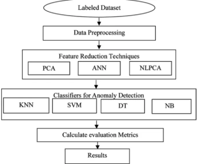
The main phases of our methodology are pre-processing, followed by feature reduction for identifying key features, and then machine learning based classification for attack detec-tion. Novel performance measures, Classifica-tion Difference Measure (CDM), Specificity Difference Measure (SPDM), Sensitivity
Dif-ference Measure (SNDM), F1 Difference
sure (F1DM) and Combined Performance Mea-sure (CPM) have been computed in this work, details of which are discussed in this section.
The main phases of the proposed methodology have been shown in Figure 1 and their detailed description is explained next.
Figure 1. Different Phases of Proposed Methodology.
3.1. Data Preprocessing
3.1.1. Preprocessing of CIDDS Dataset
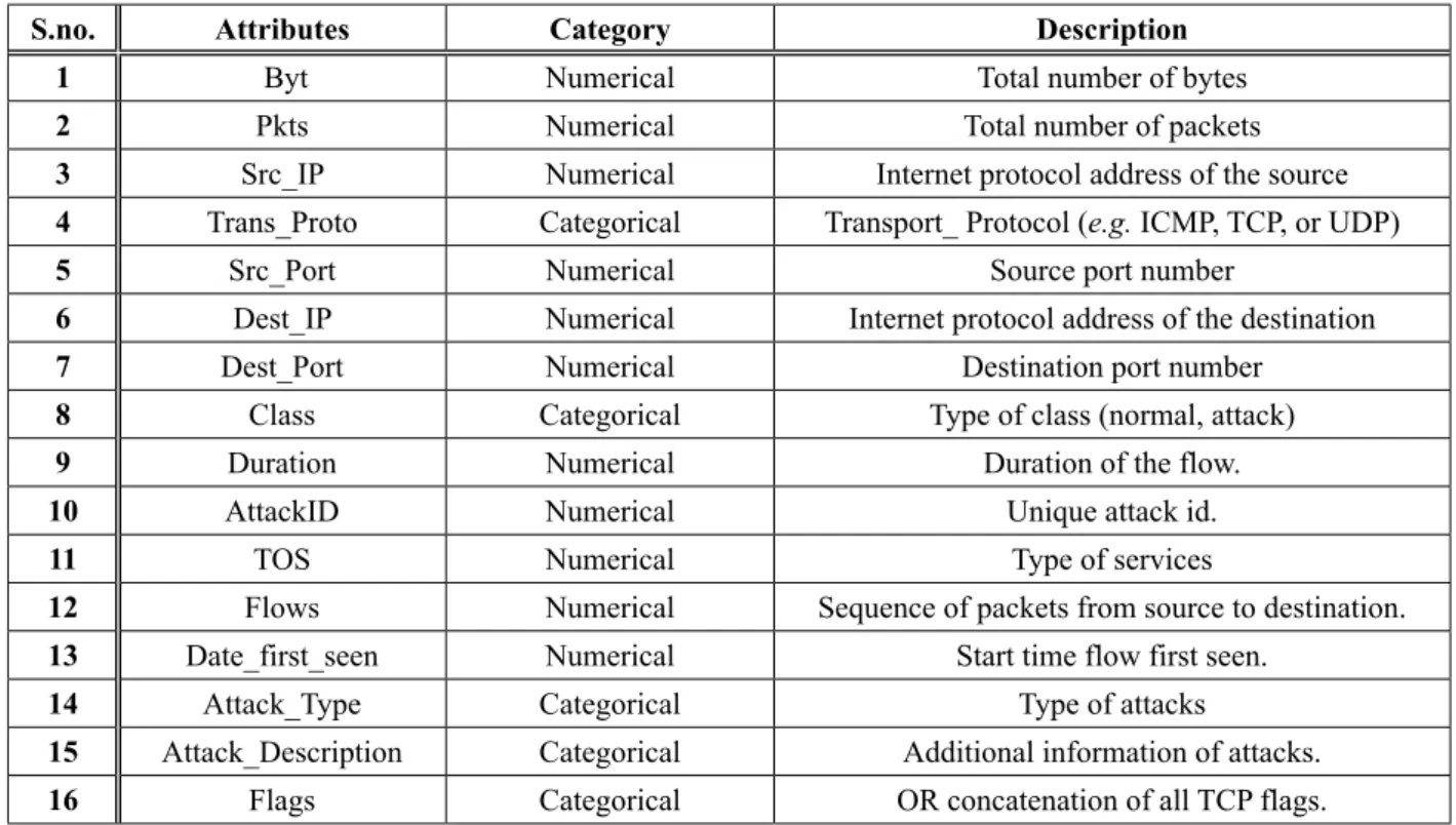
To transform captured data into a format ap-propriate for the application of machine learn-ing techniques data processlearn-ing should be per-formed. Most of the publicly available intrusion detection datasets have unwanted raw attributes which are not required for specific classifica-tion techniques. In this work, the Coburg In-trusion Detection Data Sets (CIDDS) [24] has been used for anomaly detection. The CIDDS dataset consisted of both numerical and cate-gorical attributes as shown in Table 1.
The following preprocessing steps were done on the dataset.
1. Out of these AttackID, Date_first_seen,
Duration, Attack_Type, Attack_Descrip-tion and Flags were dropped as these at-tributes did not contribute to classification. Binary data preprocessing was not required because there was no binary data.
2. Since the algorithms based on distance measure work on integer values only, we converted dotted decimal notation of Src_IP, Dest_IP to long integer (e.g.
192.16.68.44 to 192166844). There were addresses in string form to which numer-ical values were assigned (e.g. ext_server to 200000000).
Table 1. Description of Attributes of CIDDS Dataset.
S.no. Attributes Category Description
1 Byt Numerical Total number of bytes
2 Pkts Numerical Total number of packets
3 Src_IP Numerical Internet protocol address of the source
4 Trans_Proto Categorical Transport_ Protocol (e.g. ICMP, TCP, or UDP)
5 Src_Port Numerical Source port number
6 Dest_IP Numerical Internet protocol address of the destination
7 Dest_Port Numerical Destination port number
8 Class Categorical Type of class (normal, attack)
9 Duration Numerical Duration of the flow.
10 AttackID Numerical Unique attack id.
11 TOS Numerical Type of services
12 Flows Numerical Sequence of packets from source to destination.
13 Date_first_seen Numerical Start time flow first seen.
14 Attack_Type Categorical Type of attacks
15 Attack_Description Categorical Additional information of attacks.
3. Values in the 'Byt' field that were non-nu-meric like '2.1M' were converted to the in-teger form like (2.1M to 2100000).
4. In order to convert the categorical field 'Trans_Proto' to the numeric field, the following convention has been applied: TCP, ICMP, UDP, GRE were mapped to 1, 2, 3, 4, respectively.
5. 'Flows' and 'TOS' were also removed be-cause both of them had a single constant value of 1.0.
6. The CIDDS dataset consisted of parame-ters like 'Byt' where there were small num-bers of instances with a high byte count and a large number of instances with very small byte count, like 21000000,76. There-fore, normalization was applied to scale down the values into the range of zero to one based on the equation given below:
( ) ( )
n x mean x
X = −std x
(1) where x is the attribute value, std is the standard deviation and Xn is the calculated
normalized value.
7. The statistical procedure called Pearson Correlation Coefficient has been used to analyze the linearity and nonlinearity of the dataset. It quantified Byt and Pkts attri-butes as linear in nature and the remaining attributes as nonlinear.
3.1.2. Preprocessing of NSL-KDD Dataset
The KDDCUP dataset is the most preferred publicly available dataset used by the research-ers working in the field of network intrusion detection. However, Ghorbani et al. [25] per-formed a statistical analysis of this dataset and reported some inconsistencies. They found out that these irregularities could be affecting the performance of IDSs, especially the ones pre-sumed on anomaly based network intrusion de-tection. Their team removed irrelevant records from the original files and proposed a new data-set, named, NSL-KDD. The dataset has 41 fea-tures with label class as 42nd feature and has been divided into nominal, binary and numeric values. The NSL-KDD dataset files have been divided into training dataset and testing dataset. Instances in these files are 'labeled' as 'normal' for regular traffic and 'attack' for attack traffic. KNN or Decision Tree (DT) algorithms were
used for classification. Test result showed that KPCA with the proposed kernel, i.e. the pow-er kpow-ernel, ppow-erformed bettpow-er in comparison with various varieties of other kernels. In addition, the detection rate for two types of attacks, i.e. probe attacks and DOS attacks, was the highest in comparison to the PCA method. Y. Wang, H. Yao, and S. Zhao in [21] explained the concept of Auto Associative Neural Network (AANN) and focused on its ability in nonlinear feature reduction. In [22] M. A. Kramer presented a PCA technique for nonlinear feature reduction in chemical engineering, which is based on the neural network model, and referred to the result-ing technique as Non-Linear PCA (NLPCA) us-ing Auto Associative Neural Network (AANN). Kramer's NLPCA has been applied to problems in data reduction and visualization, sensor vali-dation, fault detection, quality control, principal component regression, etc. The results showed that NLPCA can be applied in a more general way than PCA. Also, NLPCA improves the per-formance of these tasks.
From the above research we observed that the majority of the respective algorithms had been tested on old and obsolete datasets. Therefore, study of the new dataset was required. The CIDDS dataset is the most recent publicly avail-able dataset [23] used by researchers working in the area of anomaly detection. Performance of the said models has been evaluated on the CIDDS dataset. Additionally, Artificial Neural Network (ANN), which was previously used for classification purposes only, was applied in feature reduction.
In the next section we discuss the proposed methodology.
3. Research Methodology
The main phases of our methodology are pre-processing, followed by feature reduction for identifying key features, and then machine learning based classification for attack detec-tion. Novel performance measures, Classifica-tion Difference Measure (CDM), Specificity Difference Measure (SPDM), Sensitivity
Dif-ference Measure (SNDM), F1 Difference
sure (F1DM) and Combined Performance Mea-sure (CPM) have been computed in this work, details of which are discussed in this section.
The main phases of the proposed methodology have been shown in Figure 1 and their detailed description is explained next.
Figure 1. Different Phases of Proposed Methodology.
3.1. Data Preprocessing
3.1.1. Preprocessing of CIDDS Dataset
To transform captured data into a format ap-propriate for the application of machine learn-ing techniques data processlearn-ing should be per-formed. Most of the publicly available intrusion detection datasets have unwanted raw attributes which are not required for specific classifica-tion techniques. In this work, the Coburg In-trusion Detection Data Sets (CIDDS) [24] has been used for anomaly detection. The CIDDS dataset consisted of both numerical and cate-gorical attributes as shown in Table 1.
The following preprocessing steps were done on the dataset.
1. Out of these AttackID, Date_first_seen,
Duration, Attack_Type, Attack_Descrip-tion and Flags were dropped as these at-tributes did not contribute to classification. Binary data preprocessing was not required because there was no binary data.
2. Since the algorithms based on distance measure work on integer values only, we converted dotted decimal notation of Src_IP, Dest_IP to long integer (e.g.
192.16.68.44 to 192166844). There were addresses in string form to which numer-ical values were assigned (e.g. ext_server to 200000000).
Table 1. Description of Attributes of CIDDS Dataset.
S.no. Attributes Category Description
1 Byt Numerical Total number of bytes
2 Pkts Numerical Total number of packets
3 Src_IP Numerical Internet protocol address of the source
4 Trans_Proto Categorical Transport_ Protocol (e.g. ICMP, TCP, or UDP)
5 Src_Port Numerical Source port number
6 Dest_IP Numerical Internet protocol address of the destination
7 Dest_Port Numerical Destination port number
8 Class Categorical Type of class (normal, attack)
9 Duration Numerical Duration of the flow.
10 AttackID Numerical Unique attack id.
11 TOS Numerical Type of services
12 Flows Numerical Sequence of packets from source to destination.
13 Date_first_seen Numerical Start time flow first seen.
14 Attack_Type Categorical Type of attacks
15 Attack_Description Categorical Additional information of attacks.
where E[fi] and E[fj] denote the expected
value of the attributes fi, fj respectively, and
1 ≤i, j≤ 7.
2. Using the covariance matrix, the eigenvec-tors and eigenvalues were calculated. 3. The obtained eigenvalues were sorted in
decreasing order as given in Table 2. These eigenvalues were used as PCs whereby the eigenvector with the highest eigenvalue
ev1 became the first principal component PC1, second highest eigenvector with the highest eigenvalue ev2 became second
principal component PC2 and so on.
4. In order to decide the sufficient number (n) of features, we performed both the Scree Plot Test and the Critical Eigenvalue Test
(Cureton and D'Agostino, 1983). The re-maining features were discarded as redun-dant data.
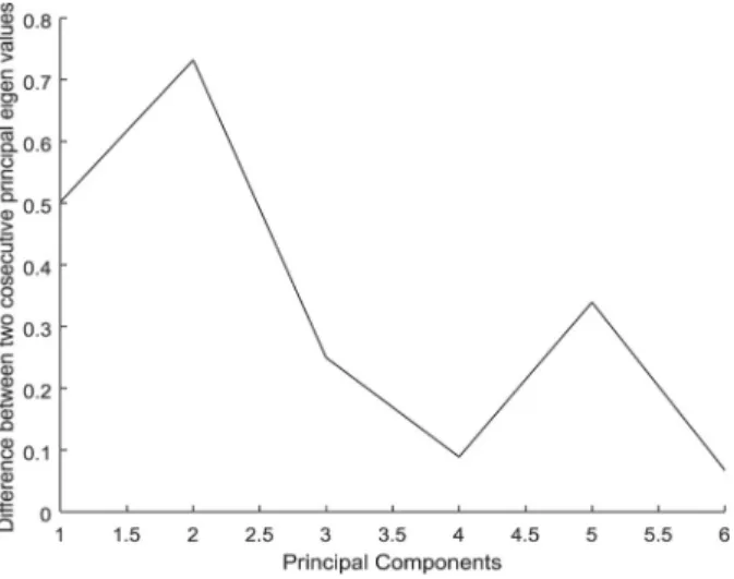
a) In Scree Plot Test, the differences di fi
between respective PCs are computed using the sorted eigenvalues.
d fi j =ev evi− i+1 (3)
A graph of principal components vs eigenvalue differences was plotted as shown in Figure 2. From the plot, peaks were observed at points dif2(0.7318)
and dif5 (0.3395). Therefore, the break
in the trend happened between points
di f2 and di f3
,
and between di f5 and di f6. Since two peak values werere-ceived, we performed another test i.e.
the critical eigenvalue test.
b) The Critical EigenvalueTest is used to compute the threshold of eigenvalues to detect the number of final principal com-ponents. Several experiments were con-ducted to determine the best threshold. For our tests we found that 0.910
c f
τ =
was appropriate, where f is a feature of the dataset. For our test, τc was 0.5762.
Based on these two tests, the number of significant features was decided to be five. These five features were Src_IP,
Trans_Proto, Src_Port, Dest_IP, and
Dest_Port.
5. The obtained five feature vectors in step 4 were used to compute new features. The
formula to calculate new features is given below:
nfx= [f1, f2, f3, f4, f5, f6, f7] ⋅ [evi, j],
for x= 1 to 5, i, j= 1 to 7 (4) PCA_DATA = {nf1, nf2, nf3, nf4, nf5, nf6, nf7},
where PCA_DATA is new dataset and nfx
is new feature.
This new dataset PCA_DATA was further used as an input to the classifiers in the next phase. Being a linear dimension reduction technique, PCA has its obvious limitation. Hence, we have used Non Linear Principal Component Analy-sis (NLPCA) using the auto-associative neural network model. The implementation of NLP-CA is presented in Section 3.2.3. Additionally, we have used the multi-layer perceptron neu-ral network called Artificial Neuneu-ral Network (ANN) model. Based on the accuracy, best at-tributes were selected. To get rid of correlations among these attributes, we again used the Auto Associative Neural Network model (AANN). The uncorrelated features, thus obtained, were used as input to classifiers. Implementation de-tails are discussed in the next section.
Figure 2. Scree Plot Test.
3.2.2. Artificial Neural Network
The Artificial Neural Network (ANN) is used to solve classification problems, noise reduc-tion, predicreduc-tion, etc. ANN helps in prediction of future score based on past knowledge and specified learning on a training dataset. In this work ANN has been used for feature reduction. 1. That dataset has six binary parameters,
namely, land, logged_in, root_shell, su_at-tempted, is_host_login, and is_guest_login
but su_attempted has 3 values (0, 1, 2). To convert su_attempted to binary values, the value 2.0 was replaced with 0.0 because there was no instance of value 2.0 in the training data and only 59 instances in the testing dataset. Therefore, it was appropri-ate to replace 2.0 with 0.0 for su_attempted
parameter.
2. It was realized that the parameter 'num_ outbound_cmds' has only 0.0 values and therefore it was decided to remove the in-stances of this parameter.
3. Since most of machine learning algorithms use numerical data for their algorithms, la-bel encoding was applied to convert cat-egorical data to integer values. Three pa-rameters, namely, Protocol_type, Service, and Flag were converted to numerical val-ues using label encoding.
4. Training data was further divided into 80:20 ratios where 20 percent was used for cross validation.
3.2. Feature Reduction Techniques
In machine learning the complexity of the al-gorithms is dependent on two characteristics of the dataset: number of input variables (i.e.
dimensions 'd') and size of the dataset (i.e. num-ber of instances 'n'). Therefore, dimensionality reduction of any of the above two characteris-tics helps in reducing space complexity. This improves the performance of machine learning algorithms. Since CIDDS dataset has very large number of instances, dimensionality reduction is crucial before applying the algorithms. Two common approaches for handling large num-ber of instances used in machine learning are: feature selection and feature reduction. Though feature selection leads to reduction in dimen-sionality by choosing a small set of attributes, this procedure is not effective in cases when all attributes are important for anomaly detection. Therefore, feature reduction was applied to CIDDS dataset to transform original attributes so as to generate other significant features.
Three feature reduction techniques, namely Principal Component Analysis (PCA), Artifi-cial Neural Network (ANN), Nonlinear Prin-cipal Component Analysis (NLPCA), were applied on the dataset. After pre-processing the CIDDS dataset consisted of seven attributes, namely Byt, Pkts, Trans_Proto (e.g. ICMP,
TCP, or UDP), Src_IP, Src_Port, Dest_IP, and,
Dest_Port.
Details of the applied feature reduction tech-nique are explained in the following.
3.2.1. Principal Component Analysis
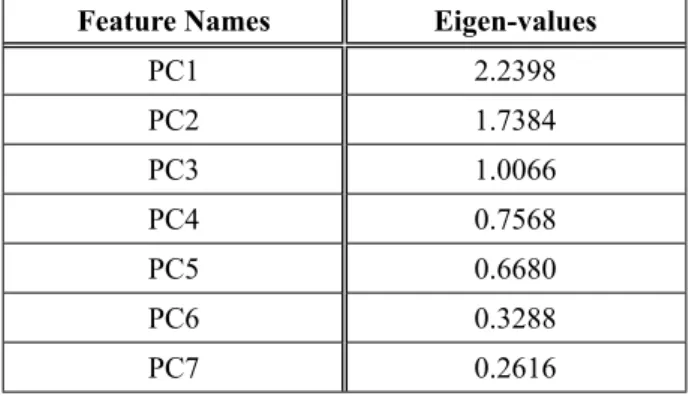
PCA works on the basis of variances. Individu-al variances for various attributes in the dataset were computed and dimensionality reduction was done based on variance score. The first five principal components, as given in Table 2, were selected with the highest variance of 91.56 percent and further used in the second step as an input vector for classifiers to per-form anomaly detection. We divided the data-set into 80:20 ratios, where 80 percent of the instances were used for training. The training data subset was used for finding out the Princi-pal Components (PCs).
Table 2. Principal Components (PCs) and Correspond-ing Eigen-Values Elected based on Outcomes of Scree
Plot Test and Critical Eigenvalue Test.
Feature Names Eigen-values
PC1 2.2398
PC2 1.7384
PC3 1.0066
PC4 0.7568
PC5 0.6680
PC6 0.3288
PC7 0.2616
The steps involved in calculating the PCs are given below.
1. The covariance of seven attributes was cal-culated based on the equation given below:
[ ]
[ ]
cov( )
, i j
i i i i
f f
E E f f E E f f
=
= − ⋅ −
where E[fi] and E[fj] denote the expected
value of the attributes fi, fj respectively, and
1 ≤i, j≤ 7.
2. Using the covariance matrix, the eigenvec-tors and eigenvalues were calculated. 3. The obtained eigenvalues were sorted in
decreasing order as given in Table 2. These eigenvalues were used as PCs whereby the eigenvector with the highest eigenvalue
ev1 became the first principal component PC1, second highest eigenvector with the highest eigenvalue ev2 became second
principal component PC2 and so on.
4. In order to decide the sufficient number (n) of features, we performed both the Scree Plot Test and the Critical Eigenvalue Test
(Cureton and D'Agostino, 1983). The re-maining features were discarded as redun-dant data.
a) In Scree Plot Test, the differences di fi
between respective PCs are computed using the sorted eigenvalues.
d fi j =ev evi− i+1 (3)
A graph of principal components vs eigenvalue differences was plotted as shown in Figure 2. From the plot, peaks were observed at points dif2(0.7318)
and dif5 (0.3395). Therefore, the break
in the trend happened between points
di f2 and di f3
,
and between di f5 and di f6. Since two peak values werere-ceived, we performed another test i.e.
the critical eigenvalue test.
b) The Critical EigenvalueTest is used to compute the threshold of eigenvalues to detect the number of final principal com-ponents. Several experiments were con-ducted to determine the best threshold. For our tests we found that 0.910
c f
τ =
was appropriate, where f is a feature of the dataset. For our test, τc was 0.5762.
Based on these two tests, the number of significant features was decided to be five. These five features were Src_IP,
Trans_Proto, Src_Port, Dest_IP, and
Dest_Port.
5. The obtained five feature vectors in step 4 were used to compute new features. The
formula to calculate new features is given below:
nfx= [f1, f2, f3, f4, f5, f6, f7] ⋅ [evi, j],
for x= 1 to 5, i, j= 1 to 7 (4) PCA_DATA = {nf1, nf2, nf3, nf4, nf5, nf6, nf7},
where PCA_DATA is new dataset and nfx
is new feature.
This new dataset PCA_DATA was further used as an input to the classifiers in the next phase. Being a linear dimension reduction technique, PCA has its obvious limitation. Hence, we have used Non Linear Principal Component Analy-sis (NLPCA) using the auto-associative neural network model. The implementation of NLP-CA is presented in Section 3.2.3. Additionally, we have used the multi-layer perceptron neu-ral network called Artificial Neuneu-ral Network (ANN) model. Based on the accuracy, best at-tributes were selected. To get rid of correlations among these attributes, we again used the Auto Associative Neural Network model (AANN). The uncorrelated features, thus obtained, were used as input to classifiers. Implementation de-tails are discussed in the next section.
Figure 2. Scree Plot Test.
3.2.2. Artificial Neural Network
The Artificial Neural Network (ANN) is used to solve classification problems, noise reduc-tion, predicreduc-tion, etc. ANN helps in prediction of future score based on past knowledge and specified learning on a training dataset. In this work ANN has been used for feature reduction. 1. That dataset has six binary parameters,
namely, land, logged_in, root_shell, su_at-tempted, is_host_login, and is_guest_login
but su_attempted has 3 values (0, 1, 2). To convert su_attempted to binary values, the value 2.0 was replaced with 0.0 because there was no instance of value 2.0 in the training data and only 59 instances in the testing dataset. Therefore, it was appropri-ate to replace 2.0 with 0.0 for su_attempted
parameter.
2. It was realized that the parameter 'num_ outbound_cmds' has only 0.0 values and therefore it was decided to remove the in-stances of this parameter.
3. Since most of machine learning algorithms use numerical data for their algorithms, la-bel encoding was applied to convert cat-egorical data to integer values. Three pa-rameters, namely, Protocol_type, Service, and Flag were converted to numerical val-ues using label encoding.
4. Training data was further divided into 80:20 ratios where 20 percent was used for cross validation.
3.2. Feature Reduction Techniques
In machine learning the complexity of the al-gorithms is dependent on two characteristics of the dataset: number of input variables (i.e.
dimensions 'd') and size of the dataset (i.e. num-ber of instances 'n'). Therefore, dimensionality reduction of any of the above two characteris-tics helps in reducing space complexity. This improves the performance of machine learning algorithms. Since CIDDS dataset has very large number of instances, dimensionality reduction is crucial before applying the algorithms. Two common approaches for handling large num-ber of instances used in machine learning are: feature selection and feature reduction. Though feature selection leads to reduction in dimen-sionality by choosing a small set of attributes, this procedure is not effective in cases when all attributes are important for anomaly detection. Therefore, feature reduction was applied to CIDDS dataset to transform original attributes so as to generate other significant features.
Three feature reduction techniques, namely Principal Component Analysis (PCA), Artifi-cial Neural Network (ANN), Nonlinear Prin-cipal Component Analysis (NLPCA), were applied on the dataset. After pre-processing the CIDDS dataset consisted of seven attributes, namely Byt, Pkts, Trans_Proto (e.g. ICMP,
TCP, or UDP), Src_IP, Src_Port, Dest_IP, and,
Dest_Port.
Details of the applied feature reduction tech-nique are explained in the following.
3.2.1. Principal Component Analysis
PCA works on the basis of variances. Individu-al variances for various attributes in the dataset were computed and dimensionality reduction was done based on variance score. The first five principal components, as given in Table 2, were selected with the highest variance of 91.56 percent and further used in the second step as an input vector for classifiers to per-form anomaly detection. We divided the data-set into 80:20 ratios, where 80 percent of the instances were used for training. The training data subset was used for finding out the Princi-pal Components (PCs).
Table 2. Principal Components (PCs) and Correspond-ing Eigen-Values Elected based on Outcomes of Scree
Plot Test and Critical Eigenvalue Test.
Feature Names Eigen-values
PC1 2.2398
PC2 1.7384
PC3 1.0066
PC4 0.7568
PC5 0.6680
PC6 0.3288
PC7 0.2616
The steps involved in calculating the PCs are given below.
1. The covariance of seven attributes was cal-culated based on the equation given below:
[ ]
[ ]
cov( )
, i j
i i i i
f f
E E f f E E f f
=
= − ⋅ −
2. A custom auto-associative neural network is created to generate nonlinear features. The network consisted of seven neurons in the input layer, and three hidden layers, namely, hidden layer 1 (HL1), bottleneck
layer (BL), and hidden layer 3 (HL3),
re-spectively. In addition, there were seven neurons in the output layer.
3. Five neurons were considered in HL1 and HL3, as explained in the ANN technique.
4. The number of neurons in the bottleneck layer varied from the number of attributes from one to seven.
5. Activation functions tan sigmoid were used in hidden layers, while pure linear
function was used in the output layer. The
trainlm function was used for training the network.
6. The output of HL1 was passed as input to BL. BL is the vital layer used for feature re-duction by eliminating nodes. The output of the bottleneck was passed to HL3.
7. Output is computed basing on the iterative pruning of the input attributes in the bot-tleneck layer, by removing attributes one by one and computing the accuracy of the training dataset. Based on the best results, the last five attributes were fixed, namely,
Src_IP, Trans_Proto, Src_Port, Dest_IP, and Dest_Port, as shown in Figure 4. 8. The output obtained from the model using
five attributes selected in step 7 was fixed as a new reduced feature to form the new dataset (NLPCA_DATA). This new data-set became the input for the classifiers.
Figure 4. Predicted accuracies over test data by pruning the BL in NLPCA.
3.3. Classifiers for Anomaly Detection
Four supervised machine learning classifiers, namely Decision Tree (DT), K Nearest Neigh-bor (KNN), Support Vector Machine (SVM), and Naïve Bayes (NB) were applied on the datasets generated in phase 3.2. This is the data from three different independent dimension reducers, while actual data is fed to the four classifiers simultaneously. Additionally, the in-formation gain was evaluated to decide on the best technique. Respective classifiers are ex-plained next.
3.3.1. Decision Tree Based Anomaly Detection
Decision Tree based classification is based on the construction of DT by deciding how the nodes are split. The vital part in DT construc-tion is splitting the node value. To decide on the splitting value, the steps followed in our algo-rithm are explained next.
1. Check the class of all instances in the data-set. If they belong to a single class, then create a single node and stop.
2. For each feature (f ) the gain ratio was computed as the ratio of feature informa-tion gain and feature split value, using the formula given below:
( ) ( )i i
information gain f
Gain Ratio= s f
(6) where, i ≤n, n is the number of features in the dataset.
3. To compute the feature information gain, individual entropy values were computed for attack and for normal classes. To com-pute the entropy, individual probabilities were calculated for all features and for two classes namely normal and attack, the for-mula use in given equation is using the fol-lowing equation:
2 1
( )
( ) log ( ) , i
k i k i
k i i
Entropy f
frequency c f c f
f f
α
=
=
= −
∑
⋅(7)
where C =C1, C2 is the set of classes, and α= number of classes.
In a three-layer perceptron ANN with nonlinear transfer function, the first layer consists of in-put attributes also called neurons, while the sec-ond layer is called hidden layer in which each neurons receive inputs from the first layer neu-ron output. The sigmoid nonlinear activation function has been used in the hidden layer for extracting significant features. The third layer is the output layer in which the identity activa-tion funcactiva-tion has been used. Its basic funcactiva-tion is defined as:
f I( )=τ
∑
j W Ij⋅ j, (5) where f(I) is the predicted output of the class label, τ is the sigmoid activation function andWj is a weight of each instance Ij
.
The steps listed below were followed for fea-ture reduction.
1. To determine the number of neurons re-quired if hidden layer accuracy rate was computed. The values were computed by taking one to five neurons at a time. So the best accuracy of 97 percent was obtained for five neurons and therefore five neurons were fixed.
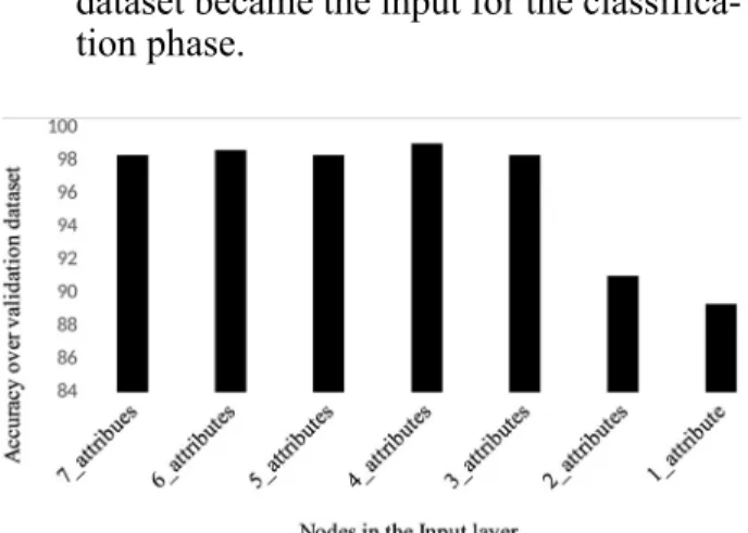
2. Since training of the network is largely de-pendent on the number of epochs required, Early Stopping Criteria (ESC) was used to determine the number of epochs. ESC is based on how accurately the training data is predicted and on the number of epochs used for achieving that accuracy. In this work different accuracy values were calcu-lated by increasing the five epochs at every step. Best accuracy (approx. 97 percent) was obtained for 40 epochs and therefore the number of epochs was fixed at 40. 3. Iterative pruning of the input attributes was
done by removing them one by one. First-ly, all seven attributes were taken, namely
Byt, Pkts, Src_IP, Trans_Proto, Src_Port,
Dest_IP, and Dest_Port, and the accuracy of the validation dataset was computed. Secondly, six attributes were taken by re-moving the first attribute which was Byt. Thirdly, five attributes were taken by re-moving the first two attributes which were
Byt and Pkts and the process was contin-ued till the best accuracy was achieved. And based on best results, the last four
attributes were fixed, namely, Trans_ Pro-to, Src_Port, Dest_IP, and Dest_Port, as shown in Figure 3.
4. In the output obtained from the model in step 3 based on accuracy memorization, four best attributes were selected. Further, to get rid of the correlations among these four attributes, we again used the ANN model on these attributes. The uncorrelat-ed features, thus obtainuncorrelat-ed in step 4, were used as a new reduced feature to form the new dataset (ANN_DATA). This new dataset became the input for the classifica-tion phase.
Figure 3. Variation in prediction accuracies of ANN works over validation data.
3.2.3. Nonlinear Principal Component Analysis
Nonlinear Principal Component Analysis (NLPCA) was introduced as a nonlinear fea-ture reduction technique by (Kramer, 1991). Auto-Associative Neural Network (AANN) is used to generate NLPCA. It is a three-hid-den-layer feed-forward neural network where the target data set is identical to the input data set and the input and output layers are con-nected via weights. One of the hidden layers of the network works as a bottleneck layer of the network, which forces the reduction of data dimensionality for data interpretation and for anomaly detection.
Steps to perform nonlinear feature reduction using AANN are given below.
2. A custom auto-associative neural network is created to generate nonlinear features. The network consisted of seven neurons in the input layer, and three hidden layers, namely, hidden layer 1 (HL1), bottleneck
layer (BL), and hidden layer 3 (HL3),
re-spectively. In addition, there were seven neurons in the output layer.
3. Five neurons were considered in HL1 and HL3, as explained in the ANN technique.
4. The number of neurons in the bottleneck layer varied from the number of attributes from one to seven.
5. Activation functions tan sigmoid were used in hidden layers, while pure linear
function was used in the output layer. The
trainlm function was used for training the network.
6. The output of HL1 was passed as input to BL. BL is the vital layer used for feature re-duction by eliminating nodes. The output of the bottleneck was passed to HL3.
7. Output is computed basing on the iterative pruning of the input attributes in the bot-tleneck layer, by removing attributes one by one and computing the accuracy of the training dataset. Based on the best results, the last five attributes were fixed, namely,
Src_IP, Trans_Proto, Src_Port, Dest_IP, and Dest_Port, as shown in Figure 4. 8. The output obtained from the model using
five attributes selected in step 7 was fixed as a new reduced feature to form the new dataset (NLPCA_DATA). This new data-set became the input for the classifiers.
Figure 4. Predicted accuracies over test data by pruning the BL in NLPCA.
3.3. Classifiers for Anomaly Detection
Four supervised machine learning classifiers, namely Decision Tree (DT), K Nearest Neigh-bor (KNN), Support Vector Machine (SVM), and Naïve Bayes (NB) were applied on the datasets generated in phase 3.2. This is the data from three different independent dimension reducers, while actual data is fed to the four classifiers simultaneously. Additionally, the in-formation gain was evaluated to decide on the best technique. Respective classifiers are ex-plained next.
3.3.1. Decision Tree Based Anomaly Detection
Decision Tree based classification is based on the construction of DT by deciding how the nodes are split. The vital part in DT construc-tion is splitting the node value. To decide on the splitting value, the steps followed in our algo-rithm are explained next.
1. Check the class of all instances in the data-set. If they belong to a single class, then create a single node and stop.
2. For each feature (f ) the gain ratio was computed as the ratio of feature informa-tion gain and feature split value, using the formula given below:
( ) ( )i i
information gain f
Gain Ratio= s f
(6) where, i ≤n, n is the number of features in the dataset.
3. To compute the feature information gain, individual entropy values were computed for attack and for normal classes. To com-pute the entropy, individual probabilities were calculated for all features and for two classes namely normal and attack, the for-mula use in given equation is using the fol-lowing equation:
2 1
( )
( ) log ( ) , i
k i k i
k i i
Entropy f
frequency c f c f
f f
α
=
=
= −
∑
⋅(7)
where C =C1, C2 is the set of classes, and α= number of classes.
In a three-layer perceptron ANN with nonlinear transfer function, the first layer consists of in-put attributes also called neurons, while the sec-ond layer is called hidden layer in which each neurons receive inputs from the first layer neu-ron output. The sigmoid nonlinear activation function has been used in the hidden layer for extracting significant features. The third layer is the output layer in which the identity activa-tion funcactiva-tion has been used. Its basic funcactiva-tion is defined as:
f I( )=τ
∑
j W Ij⋅ j, (5) where f(I) is the predicted output of the class label, τ is the sigmoid activation function andWj is a weight of each instance Ij
.
The steps listed below were followed for fea-ture reduction.
1. To determine the number of neurons re-quired if hidden layer accuracy rate was computed. The values were computed by taking one to five neurons at a time. So the best accuracy of 97 percent was obtained for five neurons and therefore five neurons were fixed.
2. Since training of the network is largely de-pendent on the number of epochs required, Early Stopping Criteria (ESC) was used to determine the number of epochs. ESC is based on how accurately the training data is predicted and on the number of epochs used for achieving that accuracy. In this work different accuracy values were calcu-lated by increasing the five epochs at every step. Best accuracy (approx. 97 percent) was obtained for 40 epochs and therefore the number of epochs was fixed at 40. 3. Iterative pruning of the input attributes was
done by removing them one by one. First-ly, all seven attributes were taken, namely
Byt, Pkts, Src_IP, Trans_Proto, Src_Port,
Dest_IP, and Dest_Port, and the accuracy of the validation dataset was computed. Secondly, six attributes were taken by re-moving the first attribute which was Byt. Thirdly, five attributes were taken by re-moving the first two attributes which were
Byt and Pkts and the process was contin-ued till the best accuracy was achieved. And based on best results, the last four
attributes were fixed, namely, Trans_ Pro-to, Src_Port, Dest_IP, and Dest_Port, as shown in Figure 3.
4. In the output obtained from the model in step 3 based on accuracy memorization, four best attributes were selected. Further, to get rid of the correlations among these four attributes, we again used the ANN model on these attributes. The uncorrelat-ed features, thus obtainuncorrelat-ed in step 4, were used as a new reduced feature to form the new dataset (ANN_DATA). This new dataset became the input for the classifica-tion phase.
Figure 3. Variation in prediction accuracies of ANN works over validation data.
3.2.3. Nonlinear Principal Component Analysis
Nonlinear Principal Component Analysis (NLPCA) was introduced as a nonlinear fea-ture reduction technique by (Kramer, 1991). Auto-Associative Neural Network (AANN) is used to generate NLPCA. It is a three-hid-den-layer feed-forward neural network where the target data set is identical to the input data set and the input and output layers are con-nected via weights. One of the hidden layers of the network works as a bottleneck layer of the network, which forces the reduction of data dimensionality for data interpretation and for anomaly detection.
Steps to perform nonlinear feature reduction using AANN are given below.
3.4. Performance Evaluation Metrics
Performance was measured in terms of perfor-mance metrics, namely Accuracy (ACC), and False Positive Rate (FPR). In addition to tradi-tional performance metrics, novel performance measures such as Classification Difference Measure (CDM), Specificity Difference Mea-sure (SPDM), Sensitivity Difference Measure
(SNDM), and F1 Difference Measure (F1DM)
have been defined and the respective results were computed. Consider True Positive values as TP, False Positive values as FP, True Nega-tive values as TN, False NegaNega-tive values as FN, then TP, FP, TN and FN can be defined as:
● TP: the total count of ''normal'' instances in the dataset correctly classified as ''normal'' instances;
● FP: the total count of ''normal'' instances in the dataset wrongly classified as ''attack'' instances;
● TN: the total count of ''attack'' instances in the dataset correctly classified as ''attack'' instances;
● FN: the count of ''attack'' instances in the dataset wrongly classified as ''normal'' in-stances.
Accuracy (ACC) and False Positive Rate (FPR) scores were calculated from these metrics based on the following equations:
TP TN ACC TP TN FP FN
FP FPR FP TN
+
= + + +
= +
(12)
To evaluate the performance of such reduced datasets with actual data, the main target was to reduce the dimensionality of the feature set (F) from 'd' to 'k' such that Fk<Fd. The difference
in the detection accuracy (ACC) for the dataset with the dimension D and the dataset with the dimension K was computed as the CDM.
CDM=ACCK-ACCD (13)
Similarly, SPDM was computed as the
differ-ence in the false positive rate of D dimensional dataset and K dimensional dataset.
SPDM=FPRK-FPRD (14)
For CDM > 0, the information gain was achieved for the reduced dataset. For CDM < 0 loss of information occurred in the reduced dataset. Additionally, SPDM > 0 resulted in gain
where-as SPDM < 0 resulted in loss for the reduced
dataset. If the values for CDM and SPDM were
zero, then information retention was achieved. The measure of sensitivity has been defined as the ratio between the number of true negative cases and the sum of false positive and true negative cases. To study the impact of sensi-tivity on actual and reduced datasets, a new metric, i.e. the difference of sensitivity was computed. Sensitivity Difference Measure (SNDM) was computed as given in the
equa-tion below:
S DMN K D
TN TN
FP TN FP TN
= + − +
(15)
The F1 measure is known to reflect the bal-ance between precision and recall. For high detection performance low values of FP and FN are considered good, thus resulting in low F1. Therefore, the F1 measure can be used to indicate the performance of detection meth-ods while its difference was used to study the impact on both original and reduced datasets. A new metric, the difference of F1 scores, was computed as the F1 Difference Measure (F1DM) as given in the equation below:
F1DM=F1DMK-F1DMD
,
(16)where,
1 2 ,
, .
Precision Recall
F Score Precision+ Recall
TP Precision TP FP
TP Recall TP FN
⋅ = ⋅
= +
= +
The results are discussed in the next section.
4. Results
Performance of an intrusion or anomaly detec-tion technique is measured based on its ability to classify normal and attack instances correctly. We have applied four classifiers, namely KNN, 4. Similarly, feature information gain is
cal-culated as is shown below:
( )
( ) ,
i
i i
information gain f f Entropy f
F =
= −
∑
(8)
where F=f1, f2, …, fn, and n is the number
of features.
5. The node splitting of the tree was done basing on the highest gain ratio for the par-ticular feature.
6. Steps 1 to 4 are repeated until no splitting is possible.
3.3.2. K-Nearest Neighbor Based Anomaly Detection
K-NN is one of the simplest supervised machine learning algorithm used for classification. It classifies a data point based on how its neigh-bours behave. K-NN stores all available cases and classifies new cases based on a similarity measure. The procedure of deriving best classifi-cation model involves the three following steps. 1. Pick the right value of K, where K is the
number of nearest neighbors, in our exper-iment we choose K= 1.
2. Calculate the similarity measure (Euclide-an dist(Euclide-ance) between all the input inst(Euclide-anc- instanc-es.
3. Sort the distances and determine the near-est neighbor based on the Kth minimum
distance.
Euclidean distances were computed using the equation:
(
)
2
1
( , ) k i i ,
i
d x y x y
=
=
∑
−(9) where xi and yi are the instances in a given set
of attributes.
Similarly, ED was calculated for new data point s x, y for all the instances in a given dataset. The new calculated value was compared with the ED of the old instances. The class of the in-stance for which the new calculated value was closest was considered as the resulting class of the new data point.
3.3.3. Support Vector Machine Based Anomaly Detection
The Support Vector Machine is a supervised machine learning technique based on classi-fication or regression in network anomaly de-tection. In network anomaly detection it is pri-marily used for classification. Using SVM, data instances are plotted as points in an n -dimen-sional space, where n is the number of features. The coordinates represent the value of each fea-ture individually. These coordinates are used for classification by finding both the hyperplane of attack and normal classes. In this work the two classes are normal class and attack class. The target was to use SVM so that the separating margin of these classes could be maximized as well as the training error could be minimized. The SVM ability to generalize the result de-pended on the margins. These coordinate points in the hyperplane were used to find the support vectors which were further used to find the hy-perplane. To do so, α coefficients for the kernel function were computed using the equation:
1
( ) ( )
(
,)
,n
i i
i
i y k x x b
α =
+
∑
(10) where, 1 ≤i≤n, xiyi is the ith coordinate, xi is an
input vector of any dimension, yi is a class label
(1 or 0), αi is the associated coefficient, k is a
kernel function that operates on two vectors and gives a scalar output, and b is a scalar value.
3.3.4. Naïve Bayes Based Anomaly Detection
For classification problems, Naïve Bayes (NB) is one of the most popular machine learning algorithms. It studies the interconnection be-tween dependent and independent features to obtain a contingent probability for every con-nection. Therefore, a strong assumption has been established that the features are indepen-dent. The mathematical representation of NB is shown below:
(
)
(
) (
)
(
)
( )
1 2 7
|
| | ... |
i
i i i
P c F
P f c P f c P f c
P F =
=
(11)
where ci represents the type of classes
(c1 = Normal and c2 =Attack), and F =f1, f2, …, fn,