QED: A Novel Quaternary Encoding to Completely Avoid Re-labeling in XML Updates

QED: A Novel Quaternary Encoding to Completely Avoid

Re-labeling in XML Updates

Changqing Li

Tok Wang Ling

Department of Computer Science, National University of Singapore, Singapore, 117543

{lichangq, lingtw}@comp.nus.edu.sg

ABSTRACT

The method of assigning labels to the nodes of the XML tree is called a labeling scheme. Based on the labels only, both ordered and un-ordered queries can be processed without accessing the original XML file. One more important point for the labeling scheme is the label update cost in inserting or deleting a node into or from the XML tree. All the current labeling schemes have high update cost, therefore in this paper we propose a novel quaternary encoding approach for the labeling schemes. Based on this encoding approach, we need not re-label any existing nodes when the update is performed. Extensive experimental results on the XML datasets illustrate that our QED works much better than the existing labeling schemes on the label updates when considering either the number of nodes or the time for re-labeling.

Categories and Subject Descriptors

H.2.4 [Database Management]: Systems –Query processing

General Terms

Algorithms, Performance.

Keywords

Dynamic XML, Labeling scheme, Update, Quaternary.

1.

INTRODUCTION

As a standard to represent and exchange data on the web, XML [7] has gained a lot of attention from both research and enterprise areas. Presently there is a lot of interest in query processing over XML that conforms to an ordered tree-structured data model. There are two main techniques, viz. structural index and labeling (numbering) scheme, to facilitate the XML queries. The structural index approaches [10, 14, 15] can help to traverse the hierarchy of XML, but this traversal is costly. The labeling scheme approaches [1, 2, 21] require smaller storage space, yet they can efficiently determine the ancestor-descendant (A-D) and parent-child (P-C) relationships between any two elements of the XML. In this paper, we focus on the labeling schemes.

If the XML is static, the current labelling schemes can efficiently process different queries. However if the XML is dynamically changed, how to efficiently update the labels of the labelling schemes becomes to an important issue.

As we know, the elements in the XML are intrinsically ordered, which is referred as document order (the element sequence in the XML). The relative order of two paragraphs in the XML is important because the order may influence the semantics, thus the standard XML query languages (e.g., XPath[5] and XQuery [6]) require the output of queries to be in document order by default. Hence it is very important to maintain the document order when the XML is updated.

Though some researches [3, 8, 17, 18, 19, 21] have been done to maintain the document order in updating, the update costs of these approaches are still expensive. Therefore in this paper we focus on how to efficiently update the XML.

The main contributions of this paper are summarized as follows:

· We propose a novel dynamic quaternary encoding (called QED) that can be applied to different labeling schemes.

· QED completely avoids the re-labeling when the XML is updated.

· We conduct comprehensive experiments to demonstrate the benefits of our QED over the previous approaches.

The rest of the paper is organized as follows. Section 2 reviews the related work. We propose our dynamic quaternary encoding in Section 3. The most important part of this paper is Section 4, in which we show that the approach proposed in this paper is much more efficient than the existing schemes in processing updates. The experimental results are illustrated in Section 5, and we conclude in Section 6.

2.

RELATED WORK

In this section, we present three families of labeling schemes, viz. containment [2, 13, 24], prefix [1, 8, 17, 19] and prime [21].

2.1

Containment Scheme

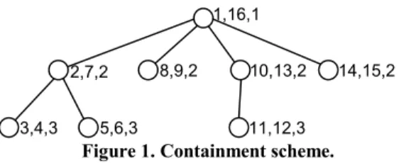
Zhang et al [24] use a labeling scheme in which every node is assigned three values: “start”, “end” and “level”. For any two nodes u and v, u is an ancestor of v iff u.start < v.start and v.end < u.end. In other words, the interval of v is contained in the interval of u. Node u is a parent of node v iff u is an ancestor of v and v.level – u.level = 1. For instance, in Figure 1, “5,6,3” is a child of “2,7,2” since interval [5, 6] is contained in interval [2, 7] and levels 3 – 2 = 1.

Permission to make digital or hard copies of all or part of this work for personal or classroom use is granted without fee provided that copies are not made or distributed for profit or commercial advantage and that copies bear this notice and the full citation on the first page. To copy otherwise, or republish, to post on servers or to redistribute to lists, requires prior specific permission and/or a fee.

CIKM’05, October 31-November 4, 2005, Bremen, Germany. Copyright 2005 ACM 1-59593-140-6/05/0010...$5.00.

Although the containment scheme is efficient to determine the ancestor-descendant relationship, the insertion of a node will lead to a re-labeling of all the ancestor nodes of this inserted node and all the nodes after this inserted node in document order (if we do not re-label, not only can not the document order be maintained, but the containment scheme can not work correctly to determine the A-D etc. relationships). This problem may be alleviated if the interval size is increased with values unused [13]. However, large interval size wastes a lot of numbers which causes the increase of storage, while small interval size is easy to lead to re-labeling. To solve the re-labeling problem, [3] uses Float-point values for the “start” and “end” of the intervals. It seems that Float-point solves the re-labeling problem [19]. But in practice, the Float-point is represented in a computer with a fixed number of bits [3, 19]. As a result, only 18 nodes can be inserted at a fixed place [3] since [3] uses the consecutive integer values at the initial labeling. Even if [3] uses values with large gaps, it still can not avoid the re-labeling due to the float-point precision. In fact, Float-point is equivalent to the method in [13] that some values are unused at the beginning. Therefore, using real values instead of integers only provides limited benefit for the node updating [19, 21].

2.2

Prefix Scheme

In the prefix labeling scheme, the label of a node is that its parent’s label (prefix) concatenates its own (self) label. For any two nodes u and v, u is an ancestor of v iff label(u) is a prefix of label(v). Node u is a parent of node v iff label(v) has no prefix when removing label(u) from the left side of label(v).

DeweyID [19] labels the nth _{child of a node with an integer n, and}

this n should be concatenated to the prefix (its parent’s label) and delimiter (e.g. “.”) to form the complete label of this child node. In practice, DeweyID uses UTF8 [23] to process the delimiter. [8] uses Binary Strings (BinaryString) to label the XML tree. When a node is inserted, DeweyID [19] and BinaryString [8] both need to re-label the sibling nodes after this inserted node and the descendants of these siblings to maintain the document order. [11] is also based on binary strings, but it is dynamic. However [11] still can not completely avoid the re-labeling due to the overflow problem (see Example 3.2).

OrdPath [17] is similar to DeweyID, but it only uses the odd numbers at the initial labeling. When the XML tree is updated, it uses the even number between two odd numbers to concatenate another odd number. When the sizes of the OrdPath codes overflow (see Example 3.2 in Section 3 for more details about the overflow problem), it must re-label all the existing nodes. [9] is similar to OrdPath [17] and [9] is not as compact as OrdPath.

2.3

Prime Scheme

Wu et al [21] use Prime numbers to label XML trees. The root node is labeled with “1” (integer). Based on a top-down approach, each node is given a unique prime number (self_label) and the label of each node is the product of its parent node’s label (parent_label) and its own self_label. For any two nodes u and v, u is an ancestor of v iff label(v) mod label(u) = 0. Node u is a parent of node v iff label(v)/self_label(v) = label(u).

Prime [21] uses SC (Simultaneous Congruence) values in Chinese Remainder Theorem [4] to determine the document order, i.e. SC mod self_label = document order. When the order is changed, Prime needs to re-calculate the SC values instead of re-labeling. Although Prime supports order-sensitive updates without any re-labeling of the existing nodes, it needs to re-calculate the SC values based on the new ordering of nodes. The re-calculation is very time consuming.

2.4

Motivation

All the current labeling schemes except Prime can not completely avoid the re-labeling in updates (OrdPath will encounter the overflow problem). Though Prime can completely avoid re-labeling, it needs to re-calculate the SC values which is much more expensive than re-labeling. Therefore the main objective of this paper is to dramatically decrease the update costs and completely avoid the re-labeling (see Sections 4.1, 5.1 and 5.2).

3.

QED ENCODING

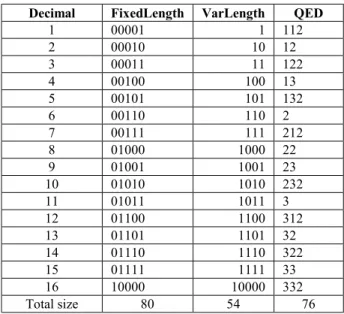
In this section, we elaborate our Quaternary Encoding for Dynamic XML data (QED) which supports label insertion without re-labeling or re-calculation (see Section 4.1). For the containment scheme shown in Figure 1 (Section 2.1), the “start” and “end” values are from 1 to 16. These decimal numbers can be encoded in binary codes with fixed length, called FixedLength1

(FixedLength column of Table 1) or with variable length, called VarLength (VarLength column of Table 1).

Definition 3.1 (Quaternary code)Four numbers “0”, “1”, “2”

and “3” are used in the code and each number is stored with two bits, i.e. “00”, “01”, “10” and “11”.

Definition 3.2 (QED code)QED code is a quaternary code. The number “0” is used as the separator and only “1”, “2” and “3”

are used in the QED code itself.

Now let us discuss how to encode the “start”s and “end”s (1-16) using our QED encoding (16 is only an example for the tree in Figure 1; our QED encoding can be applied to any other numbers; see the formal algorithm in Section 3.1). The following steps show the details of how to get the QED codes in Table 1 and these steps are examples for the formal algorithms in Section 3.1.

Step 1: In the encoding of the 16 numbers, we suppose there is one more number before number 1, say number 0, and one more number after number 16, say number 17.

1 _{Float-point, DeweyID, OrdPath, Prime, FixedLength and}

VarLength are all existing schemes. QED-PREFIX and QED (with all fonts capitalized) are schemes proposed in this paper.

Figure 1. Containment scheme.

1,16,1

2,7,2 8,9,2 10,13,2 14,15,2

Table 1. Binary and our QED encoding approaches Decimal FixedLength VarLength QED

1 00001 1 112 2 00010 10 12 3 00011 11 122 4 00100 100 13 5 00101 101 132 6 00110 110 2 7 00111 111 212 8 01000 1000 22 9 01001 1001 23 10 01010 1010 232 11 01011 1011 3 12 01100 1100 312 13 01101 1101 32 14 01110 1110 322 15 01111 1111 33 16 10000 10000 332 Total size 80 54 76

Step 2: The (1/3)th _{number is encoded with “2”, and the (2/3)}th

number is encoded with “3”. The (1/3)th _{number is number 6,}

which is calculated in this way, 6 = round(0+(17–0)/3). The (2/3)th _{number is number 11 (11 = round(0+(17–0)´2/3)).}

Step 3: The (1/3)th _{and (2/3)}th _{numbers between number 0 and}

number 6 are number 2 (2 = round(0+(6–0)/3)) and number 4 (4 = round(0+(6–0)´2/3)). The QED code of number 0 (left code) is now empty with size 0 and the QED code of number 6 (right code) is now “2” with size 1 (here 1 refers to 2 bits). This is Case (a) where the left code size is smaller than the right code size. In this case, the (1/3)th _{code is that we change the last symbol of the}

right code to “1” and concatenate one more “2”, i.e. the code of number 2 is “12” (“2”®“1” and “1”Å“2”®“12”), and the (2/3)th _{code is that we change the last symbol of the right code to}

“1” and concatenate one more “3”, i.e. the code of number 4 is “13” (“2”®“1” and “1”Å“3”®“13”).

Step 4: The (1/3)th _{and (2/3)}th _{numbers between numbers 6 and 11}

are numbers 8 (8 = round(6+(11–6)/3)) and 9 (9 = round(6+(11– 6)´2/3)). The QED code of number 6 (left code) is “2” with size 1 (here 1 refers to 2 bits) and the code of number 11 (right code) is “3” with size 1 (here 1 refers to 2 bits). This is Case (b) where the left code size is larger than or equal to the right code size. In this case, the (1/3)th _{code is that we directly concatenate one}

more “2” after the left code, i.e. the code of number 8 is “22” (“2”Å“2”®“22”), and the (2/3)th _{code is that we directly}

concatenate one more “3” after the left code, i.e. the code of number 9 is “23” (“2”Å“3”®“23”).

Step 5: The (1/3)th _{and (2/3)}th _{numbers between numbers 11 and}

17 are numbers 13 (13 = round(11+(17–11)/3)) and 15 (15 = round(11+(17–11)´2/3)). The code of number 11 (left code) is “3” with size 1 and the code of number 17 (right code) is empty now with size 0. This is still Case (b). Therefore the QED code of number 13 is “32” (“3”Å“2”®“32”), and the code of number

15 is “33” (“3”Å“3”®“33”).

In this way, all the numbers will be encoded. Finally we need to discard the codes for numbers 0 and 17 since they do not exist actually. It should be noted that Step 1 is not compulsory, but with Step 1 the total code size is smaller. It should be noted also that if the (2/3)th _{number exactly refers to the (1/3)}th _{number, the code}

for the (2/3)th _{number will not appear since this number has}

already been encoded with the (1/3)th _code.

With the following example illustration for the total code size, the formal size analysis in Section 3.2 will be easier to understand.

Example 3.1 Table 1 shows that VarLength has smaller total code size than FixedLength. However, we also need to store the size of each VarLength code, e.g., the size of “10000” is 5. We need to store this 5 using fixed length of bits (“101”; 3 bits). The sizes of other codes should also be stored using fixed length of bits (3 bits), therefore the total code size for VarLength is 3´16+54=102 bits which is larger than the bits required by FixedLength.

Example 3.2 The size of each VarLength code is stored with fixed length (e.g. 3), therefore if many nodes are inserted into the XML tree, the fixed length size (e.g. 3) is not enough for the new labels, then we have to re-label all the existing nodes. Even if we increase the size 3 to a larger number, it still can not completely avoid the re-labeling, and it will waste the storage space. This is called the overflow problem in this paper. Similarly FixedLength and OrdPath [17] will encounter the overflow problem.

Example 3.3 On the other hand, our QED uses the separator “0” (2 bits) to separate different codes instead of storing the sizes of the codes. For example, “1120120” will be separated to “112” and “12”. Therefore the size of our QED is 2´16+76=108 bits. Each size code of VarLength is stored with 3 bits, and this 3 will increase as the number of nodes increases, but the size 2 (bits) of our separator “0” will never increase. More important, we will never encounter the overflow problem in this way.

The most important feature of our QED is that it is based on the lexicographical order (for efficient updates in Section 4.1).

Definition 3.3 (Lexicographical order



(a) “0”“1” “2” “3”, or

(b) compare CA and CB symbol by symbol from left to right. If the current symbol SA of CA and the current symbol SB of CB satisfy condition (a), then CA  CB and stop the comparison, or

(c) CA is a prefix of CB.

Theorem 3.1Our QED codes are lexicographically ordered but not numerically ordered.

Example 3.4 The QED codes in Table 1 are lexicographically ordered from top to bottom. For example, “132”



“1”, while the 1st _{symbol of “2” is “2”. Another example, “23”}

_

“232” because “23” is a prefix of “232”.

When we replace the “start”s and “end”s (1-16) in Figure 1 with our QED codes, and based on the lexicographical comparison, a QED containment scheme is formed.

3.1

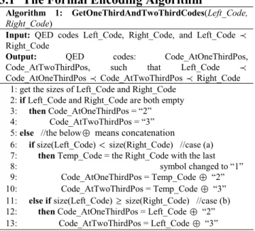
The Formal Encoding Algorithm

Algorithm 1: GetOneThirdAndTwoThirdCodes(Left_Code, Right_Code)

Input: QED codes Left_Code, Right_Code, and Left_Code  Right_Code

Output: QED codes: Code_AtOneThirdPos, Code_AtTwoThirdPos, such that Left_Code  Code_AtOneThirdPos  Code_AtTwoThirdPos  Right_Code 1: get the sizes of Left_Code and Right_Code

2: if Left_Code and Right_Code are both empty 3: then Code_AtOneThirdPos = “2”

4: Code_AtTwoThirdPos = “3”

5: else //the belowÅ means concatenation

6: if size(Left_Code) < size(Right_Code) //case (a) 7: then Temp_Code = the Right_Code with the last 8: symbol changed to “1”

9: Code_AtOneThirdPos = Temp_Code Å “2”

10: Code_AtTwoThirdPos = Temp_Code Å “3”

11: else if size(Left_Code) ³ size(Right_Code) //case (b) 12: then Code_AtOneThirdPos = Left_Code Å “2”

13: Code_AtTwoThirdPos = Left_Code Å “3”

Figure 2. GetOneThirdAndTwoThirdCodes algorithm.

Algorithm 2: Encoding(TN) Input: A positive integer TN

Output: The QED codes for numbers 1 to TN

1: suppose there is one more number before the first number, called number 0, and one more number after the last number, called number (TN+1)

2: SubEncoding(codeArr, 0, TN+1)

//here codeArr is an array with size TN+2 3: discard the 0th _{and (TN+1)}th _{elements of the array codeArr} Procedure SubEncoding(codeArr, PL, PR)

/*SubEncoding is a recursive procedure; codeArr is an array, PL is

the left position, and PR is the right position*/

4: PM1 = PL+round((PR-PL)/3) (PM1 is the (1/3)th _position) 5: PM2 = PL+round((PR-PL)´2/3) (PM2 is the (2/3)th _position) 6: if PL

¹

7: then GetOneThirdAndTwoThirdCodes(codeArr[PL], codeArr[PR]) 8: if PM1¹PL and PM1¹PR

9: then codeArr[PM1]=Code_AtOneThirdPos //from line 7 10: if PM2¹PM1 and PM2¹ PR

11: then codeArr[PM2]=Code_AtTwoThirdPos //from line 7 12: if (PM1¹PL and PM1¹PR) or (PM2¹PL and PM2¹PR) 13: then SubEncoding(codeArr, PL, PM1)

14: SubEncoding(codeArr, PM1, PM2) 15: SubEncoding(codeArr, PM2, PR)

Figure 3. QED encoding algorithm.

Algorithm 1 and Algorithm 2 are a summary of Step 1 to Step 5 (in the previous page) which can be used to encode any total number (not only 16). Here we do not explain them in detail.

3.2

Size Analysis

The size in this paper refers to bits. The log in this paper is used as the logarithm to base 2. The log3 in this paper is

used as the logarithm to base 3.

In this section, we analyze the size required by Prime, Float-point, FixedLength, VarLength and our QED. The “D” and “N” are respectively used to denote the maximal depth and the number of nodes of an XML tree.

Prime According to the size analysis of Prime in [21], the size required to store all the nodes in the XML tree is:

)) log( log(N N D

N´ ´ ´ (1)

Float-point According to [3], each float-point number is stored with 64 bits, thus the size of Float-point:

64

2N´ (2)

FixedLength The size of FixedLength is: )) 2 log(log( ) 2 log( 2N N + N ) 1 ) log(log( 2 ) log( 2 + + + = N N N N (3) )) 2

log(log( N is the size of label size (stored only once).

VarLength For VarLength, one number 1 is stored with one bit (see VarLength column of Table 1), two numbers 2 and 3 are stored with 2 bits, four numbers 4, 5, 6 and 7 are stored with 3 bits, ···, thus the total size of VarLength is:

) 1 ( 2 4 2 3 2 2 2 1 1_{´ + ´ +} 2_{´ +} 3_{´ +× ××+} n_{´ n+} 1 2 1₊ ´ =_n n+ ₍₄₎

Since the number of nodes is N, the number of “start”s and “end”s is 2N which should be equal to 20₊21_{+× ××+}2n₌2n+1_-1_. However 2N is an even number and can not be equal to 2n+1_-1_. We assume that there are 2N+1 numbers. After getting the VarLength codes, we can discard one number, i.e. 2N numbers are left. There is only a constant difference between 2N and 2N+1, thus we assume that 2N+1=2n+1_-1_{, then formula (4)} becomes: 2Nlog(N+1)+2log(N+1)+1 (5) Note that formula (5) is a little larger than the actural size required by VarLength.

We need to store the size of each “start” and “end”. A fixed-length number is used to store the size of the VarLength code. The maximal size for a “start” or an “end” is _log(2N). To store this size, the bits required are _log(log(2N)), then the total bits required to store the sizes of VarLength codes are

)) 2 log(log(

2N N . When taking formula (5) into account, the total size of VarLength is:

1 ) 1 log( 2 ) 1 log( 2 )) 2 log(log( 2N N + N N+ + N+ + (6)

QED When considering our QED, it has two numbers 6 and 11 stored with size 1 (2 bits), 6 numbers 2, 4, 8, 9, 13 and 15 stored with size 2 (2 bits), ···, therefore its size is:

+ ´ ´ ´ + ´ ´ ´ + ´ ´ ´3 ) (1 2) (2 3) (2 2) (2 3 ) (3 2) 2 ( 0 1 2 × ××+(2´3n)´((n+1)´2) _(bits) 1 3 ) 1 2 ( _{+ ´} 1₊ = _n n+ ₍₇₎ We assume 2_N=(2_´30)₊(2_´31)_{+ × ××+(2´3}n₎₌₃n+1_{-1 (both}

N N

N

Nlog (2 1) 2log (2 1) 2

4 3 + + 3 + - (8)

When considering the separator (“0”) size 2N´2, the total label size of our QED is:

N N

N

Nlog (2 1) 2log (2 1) 2

4 3 + + 3 + + (9)

It can be seen that VarLength has larger label size than FixedLength. Prime has larger size than VarLength. To make the size of Float-point smaller than VarLength, N should be grossly larger than 264_{, but generally speaking, an XML file can not have}

so many nodes. That is to say, Float-point has larger label size than VarLength. If N>264_{, 64 bits are not enough to store the}

Float-point values.

When N=1, the size of our QED is 1.6 times of that of VarLength; when NÎ_[2,7], the multiple is between 1.16 and 1.28; when

] 38 , 8 [ Î

N , the multiple is between 1.12 and 1.15; when ] 10000000 , 39 [ Î

N , the multiple is between 1.11 and 1.13. Thus the size of our QED is only a little larger than the size of VarLength.

Also we need to consider the “level” size for the containment schemes which is _Nlog(D)+_log(log(D)) and should be added into formulas (2), (3), (6) and (9) to form the total label sizes of these schemes.

Note that for simplicity, we omit the ceiling functions on the log functions in all the formulas.

3.3

Application Scope of QED

Property 3.1 Our QED is orthogonal to specific labeling schemes, thus it can be applied to all the labeling schemes or other applications which need to maintain the order.

Our QED encoding can be applied to the prefix scheme and prime scheme also to maintain the document order. When QED is applied to prefix, we call it QED-PREFIX.

Example 3.5 Figure 4 shows that we apply QED to the prefix scheme. The root has 4 children. To encode 4 numbers based on our QED, the codes will be “12”, “2”, “3” and “32”. Similarly if there are two siblings, their self_labels are “2” and “3”. If there is only one sibling, its self_label is “2”.

For the prefix scheme, the delimiter “.” can not be stored together with the numbers in the implementation to separate different components.

For our QED encoding, we use the following approach to process the delimiters. We use one separator “0” as the delimiter to separate different components of a label (e.g. separate “12” and “3” in “12.3”; the separator “0” is equivalent to the “.” in Figure 4), and use two consecutive separators “00” as the separator to separate different labels (e.g. separate “12.2” and “12.3”).

We can apply our QED to the prime labeling scheme also to record the document order. But because Prime employs the modular and division operations to determine the ancestor-descendant etc. relationships, its query efficiency is quite bad. Thus we do not discuss in detail how QED is applied to Prime. Similarly we can and it is better to apply our QED to the P-Containment scheme proposed in [12] to completely avoid re-labeling.

4.

UPDATE

In Section 4.1, we show that our QED has much cheaper update cost. Section 4.2 analyzes the case for the frequent update.

4.1

Avoid Re-labeling in Updates

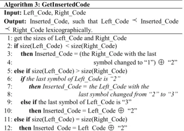
The deletion of a node will not affect the ordering of the nodes in the XML tree. Thus in this section, we only discuss the insertion. Algorithm 3 is similar to Algorithm 1, and their difference is marked in Figure 5 with italic fonts. Based on Algorithm 3, we can avoid the re-labeling. As the QED codes are long which can not be put in Figures 6, we still use decimal numbers in Figure 6 for the “start” and “end” values, but in practice, these numbers are stored using our QED codes. Refer to Table 1 for the mappings between the decimal numbers and our QED codes. We use an example to show how Algorithm 3 works.

Example 4.1 When inserting node “a” (see Figure 6), we should insert a number between the “start” of the parent “1”(Left_Code) and the “start” of the first sibling “2” (Right_Code). If we use the traditional approach, we can not insert a number between “1” and “2”, and we must re-label the nodes. However, when referring to Table 1, our QED codes for “1” and “2” are “112” and “12”. Based on the GetInsertedCode algorithm, we insert a value between “112” and “12”, then the “start” value of the inserted node “a” is “113” (see lines 5-8 of the GetInsertedCode algorithm in Figure 5). The “end” value of node “a” is an insertion between the new “start”“113” and the “start” of the first sibling “12”, thus the “end” value of “a” is “1132” (see lines 5, 9 and 10 in Figure 5). Obviously, “112”  “113”  “1132”  “12” lexicographically. We need not re-label any existing nodes, but we can keep the containment scheme working correctly.

Algorithm 3: GetInsertedCode Input: Left_Code, Right_Code

Output: Inserted_Code, such that Left_Code





1: get the sizes of Left_Code and Right_Code 2: if size(Left_Code) < size(Right_Code)

3: then Inserted_Code = (the Right_Code with the last 4: symbol changed to “1”)

Å

5: else if size(Left_Code) > size(Right_Code) 6: if the last symbol of Left_Code is “2”

7: then Inserted_Code = the Left_Code with the 8: last symbol changed from “2” to “3”

9: else if the last symbol of Left_Code is “3”

10: then Inserted_Code = Left_Code

Å

11: else if size(Left_Code) = size(Right_Code) 12: then Inserted_Code = Left_Code

Å

Figure 5. GetInsertedCode algorithm. Figure 4. QED-PREFIX scheme.

12 2 3 32

Theorem 4.1 Algorithm 3 guarantees that infinite number of QED codes can be inserted between any two consecutive QED codes with the orders kept and without any re-encoding of the existing numbers.

Based on Theorem 4.1, the insertions of nodes “b”, “c” and “d” will not cause any re-labeling also. After insertion, the level values of “a”, “b” and “c” are still 2 (2 is a decimal number for illustration), but the level value of node “d” is 3.

Now let us study the updates based on other schemes.

Example 4.2 For the containment schemes FixedLength and VarLength, when “a” is inserted into the XML tree in Figure 6, all the “start” and “end” values except the “start” value of the root need to be added with 2. The “end” value of the root will be “18” after update. It is similar for “b”, “c” and “d”.

Example 4.3 For the prefix schemes, our QED-PREFIX also need not re-label any existing nodes. DeweyID has to re-label all the sibling nodes after the inserted node and the descendants of these following sibling nodes. For Prime, the insertion of nodes will make the document order change (the orders of the nodes after this inserted node should all be added with 1), therefore Prime has to re-calculate the SC values.

Sometimes Float-point [3] and OrdPath [17] also need not re-label the nodes. Sections 5.1 and 5.2 are the update performance comparisons among Float-point, OrdPath and our approach.

4.2

Frequent Update

The size analysis in Section 3.2 is based on the initial labeling of the XML. Our encoding algorithm (see Figure 3) is step by step insertions of nodes uniformly at different places. Therefore if a sequence of nodes are inserted randomly at different places of the XML, the size analysis in Section 3.2 is still valid.

For the case that nodes are always inserted at a fixed place of the XML, the size of our QED increases quickly. [8] proves that any deterministic labeling scheme which does not re-label nodes must in the worst case assign labels of size Omega(N). Our QED can not escape from this claim also, i.e. the label size of our QED increases linearly in the worst case. OrdPath [17] also has this skewed insertion problem. [18] uses B-tree to balance the update

and lookup performance which can be used to process this skewed insertion problem. The skewed insertion is not an emphasis of this paper. In this paper, we mainly focus on how to completely avoid the re-labeling.

5.

PERFORMANCE STUDY

In this section, we evaluate and compare the performance of different labeling schemes. All the schemes are implemented in Java and all the experiments are carried out on a 3.0 GHz Pentium 4 processor with 1 GB RAM running Windows XP Professional. Table 2 shows the characteristics of the test datasets. D1, D2 and D3 are from [16], D5 and D6 are from [20], and all of them are real-world XML data. D4 is a benchmark generated by XMark [22].

Static XML is not the emphasis of this paper. However, we also test how our QED works on the static XML data which shows that our QED works not worse even in the static environment of XML (its label sizes are small in the six datasets shown in Table 2 and its query performance is not worse).

For the dynamic XML, in Section 5.1 we show that our QED works much better compared to the existing labeling schemes except OrdPath and Float-point. Although it seems that OrdPath and Float-point also work well in the intermittent insertions, the wide update performance difference between OrdPath and our QED-PREFIX, and between Float-point and our QED can be seen from Section 5.2, where frequent updates are performed.

OrdPath and our QED-PREFIX are prefix schemes. Float-point, FixedLength, VarLength, and our QED are containment schemes.

5.1

Intermittent Update

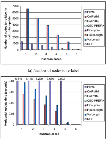
We select one XML file Hamlet in D2 to test the update performance (it is similar for other XML files). Hamlet has 5 act elements. We test the following six cases: inserting an act before act[1], inserting an act between act[1] and act[2], ···, inserting an act between act[4] and act[5], and inserting an act after act[5]. Figure 7(a) shows the number of nodes for re-labeling when applying different labeling schemes. FixedLength and VarLength have the same number of nodes to re-label in all the six cases. For case 1, 6596 (total 6636) nodes need to be re-labeled.

For Prime, the number of SC values that are required to re-calculate is counted in Figure 7(a). Because Prime uses each SC value for every five labels [21], the number of SC values required to re-calculate is 1/5 of the number of nodes required by FixedLength and VarLength to re-label. Note that it is impossible to use a single SC value for all the nodes in the XML since the SC value will be too large.

Table 2. Test datasets Datasets Topics # of files Max/average

fan-out for a file

Max/average depth for a file

Total # of nodes for each dataset

D1 Company 24 529/135 5/3 161576 D2 Shakespeare’s play 37 434/48 6/5 179689 D3 NASA 1882 1188/9 7/5 370292 D4 XMark 1 25500/3242 12/6 1666315 D5 Treebank 1 56384/1623 36/8 2437666 D6 DBLP 1 328858/65930 6/3 3332130 1,16,1 14,15,2 a b c d 2,7,2 8,9,2 10,13,2 3,4,3 5,6,3 11,12,3 Figure 6. Update.

0 1000 2000 3000 4000 5000 6000 7000 1 2 3 4 5 6 Insertion cases N u m b er o f n o d es t o r e-la b el i n h o ri zo n ta l u p d at e Prime OrdPath1 OrdPath2 QED-PREFIX Float-point FixedLength VarLength QED

(a) Number of nodes to re-label

3.616 5.229 6.148 6.841 2.093 0 0.01 0.02 0.03 0.04 1 2 3 4 5 6 Insertion cases H o ri zo n ta l u p d at e ti m e (s ec o n d s) Prime OrdPath1 OrdPath2 QED-PREFIX Float-point FixedLength VarLength QED (b) Time to re-label

Figure 7. Performance study on intermittent update.

In all the six cases, OrdPath1 (without overflow here), OrdPath2 (without overflow here), our QED-PREFIX, Float-point (less than 18 nodes), and our QED need not re-label any existing nodes. Next we study the time required to re-label nodes or re-calculate SC values. Figure 7(b) shows that the time required by Prime to re-calculate the SC values is much larger (more than 202 times; sum time of Case 1 to Case 6) than the time required by FixedLength and VarLength to re-label the nodes. Prime theoretically is a good scheme in updating order-sensitive nodes, but it is not practicable. In contrast, our QED-PREFIX and QED need less than 0.001 second (processing time) for the insertion in all the 6 cases. The processing time of FixedLength or VarLength is at least 84 times of that of QED-PREFIX and QED even if we assume that our QED needs 0.001 second for the update (in fact, it will be much larger than 84 times; see Section 5.2).

It can be seen that OrdPath1, OrdPath2 and Float-point also need less than 0.001 second for the update. This is because only several nodes are inserted into the XML. The update performance difference among OrdPath, Float-point and our approach can be seen in Section 5.2 where frequent insertions are executed.

5.2

Frequent Update

When intermittent nodes are inserted into the XML, Prime, FixedLength and VarLength have much larger update time, thus it

will be a disaster for them to update the XML with frequent and tiny insertions, which makes them impossible to answer any queries in either the uniformly frequent or skewed frequent insertion environment. In this section, we mainly compare the update performance between OrdPath and our QED-PREFIX, and between Float-point and our QED. Section 5.2.1 discusses the case that frequent insertions are randomly at different places of the XML. Section 5.2.2 discusses the worst case that frequent insertions are always at a fixed place of the XML.

5.2.1

Uniformly Frequent Update

In this section, we test the uniformly distributed frequent insertions. The Hamlet file has totally 6636 nodes. We insert 6635 nodes between every two consecutive nodes of the 6636 nodes. Based on the new file after insertion, we insert another 13270 nodes between any two consecutive nodes. We repeat this kind of insertion 6 times. After the 6th _{time insertion, the node number in}

Hamlet is 424641 that is 63.99 times of the original node number. The first two time insertions and the first four time insertions respectively will not cause OrdPath [17] (without overflow) and Float-point [3] (less than 18 nodes at a fixed place) to re-label the existing nodes. Even without re-labeling, Figure 8(a) shows that the update time of OrdPath is still at least 529 times of that of our QED-PREFIX and Figure 8(b) shows that the update time of point is 386 times of that of our QED. OrdPath and Float-point have much larger update time because they need the addition and division operations to get the numbers between two numbers which are very expensive. On the other hand, our QED-PREFIX and QED only need to modify the last quaternary number (two bits) of the neighbor label to get the label of the inserted node which is much cheaper.

At the 3rd _{time insertion, OrdPath needs to re-label all the existing}

nodes, and at the 5th _{and 6}th _{time insertions, Float-point needs to}

re-label all the existing nodes. The re-labeling time of OrdPath and Float-point is at least 2492 times of that of our QED-PREFIX and QED (see Figures 8(a) and 8(b)).

5.2.2

Skewed Frequent Update

In this section, we test the case that nodes are always inserted at a fixed place of the Hamlet XML.

Figure 9 shows the labeling time (the update time without re-labeling in skewed frequent insertions is similar to the update time shown in Figure 8). For OrdPath (OrdPath1 and OrdPath2) [17], after inserting 163 nodes at the fixed place, it needs to re-label 5 times. The re-labeling time of OrdPath is at least 8126 times of that of our QED-PREFIX (see Figure 9(a)). When every 18 nodes are inserted at the fixed place of the XML, Float-point [3] needs to re-label. The update time of Float-point is 34383 times of that of our QED after 199 nodes are inserted (see Figure 9(b)). The very large update time makes OrdPath and Float-point unsuitable to answer queries no matter in the uniformly or in the skewed frequent insertion environment. This means even if we do not use any skeweness processing technique, our QED still works the best to answer queries in the environment that frequent insertions are executed.

For the frequent update, our QED-PREFIX and QED have much cheaper update cost than OrdPath and Float-point.

0 100 200 300 400 500 600 0 150000 300000 450000

Number of nodes inserted

U p d at e ti m e fo r b al an ce d t in y in se rt io n s (s ec o n d s) OrderPath1 OrderPath2 QED-PREFIX

(a) OrdPath1&2 vs QED-PREFIX 0 1000 2000 3000 4000 5000 6000 7000 8000 9000 0 150000 300000 450000

Number of nodes inserted

U p d at e ti m e fo r b al an ce d t in y in se rt io n s (s ec o n d s) Float-point QED (b) Float-point vs QED 0 2 4 6 8 10 12 0 50 100 150 200

Number of nodes inserted

U p d at e ti m e w it h r e-la b el in g f o r sk ew ed t in y in se rt io n s (s ec o n d s) OrdPath1 OrdPath2 QED-PREFIX

(a) OrdPath1&2 vs QED-PREFIX 0 30 60 90 120 150 0 50 100 150 200

Number of nodes inserted

U p d at e ti m e w it h r e-la b el in g f o r sk ew ed t in y in se rt io n s (s ec o n d s) Float-point QED (b) Float-point vs QED

Figure 8. Performance study on uniformly frequent update. Figure 9. Performance study on skewed frequent update.

6.

CONCLUSION

In this paper, we have proposed a novel Dynamic Quaternary Encoding (QED) approach for the labeling schemes. This encoding approach is orthogonal to specific labeling schemes, therefore it can be applied broadly to different labeling shemes, e.g. containment, prefix and prime schemes, to maintain the document order when the XML is updated.

The QED (or QED-PREFIX) proposed in this paper completely (no overflow) avoids the re-labeling in XML update. When a node is inserted, our QED (or QED-PREFIX) only needs to modify the last quaternary number (two bits) of the neighbor label to get the label of the inserted node which is very easy and cheap compared to Float-point (or OrdPath). The experimental results show that our QED (or QED-PREFIX) encoding is the only approach which supports frequent insertions efficiently.

7.

REFERENCES

[1] S. Abiteboul, H. Kaplan, and T. Milo. Compact labeling schemes for ancestor queries. In Proc. SODA, pages 547-556, 2001.

[2] R. Agrawal, A. Borgida, and H.V. Jagadish. Efficient Management of Transitive Relationships in Large Data and Knowledge Bases. In Proc. of SIGMOD, pages 253-262, 1989.

[3] T. Amagasa, M. Yoshikawa, and S. Uemura. QRS: A Robust Numbering Scheme for XML Documents. In Proc. of ICDE, pages 705-707, 2003.

[4] J.A. Anderson and J.M. Bell. Number Theory with Application. Prentice-Hall, New Jersey, 1997.

[5] A. Berglund, S. Boag, D. Chamberlin, M. F. Fernandez, M. Kay, J. Robie, and J. Simon. XML path language (XPath) 2.0. W3C working draft 04, Apr 2005.

[6] S. Boag, D. Chamberlin, M. F. Fernandez, D. Florescu, J. Robie, and J. Simon. XQuery 1.0: An XML Query Language. W3C working draft 04, Apr 2005.

[7] T. Bray, J. Paoli, C. M. Sperberg-McQueen, E. Maler, and F. Yergeau. Extensible markup language (XML) 1.0 third edition W3C recommendation. Oct. 2000.

[8] E. Cohen, H. Kaplan, and T. Milo. Labeling Dynamic XML Trees. In Proc. of PODS, pages 271-281, 2002.

[9] M. Duong and Y. Zhang. A New Labeling Scheme for Dynamically Updating XML Data. In Proc. of ADC, pages 185-193, 2005.

[10]R. Goldman and J. Widom. DataGuides: Enabling Query Formulation and Optimization in Semistructured Databases. In Proc. of VLDB, pages 436-445, 1997.

[11]C. Li and T.W. Ling. An Improved Prefix Labeling Scheme: A Binary String Approach for Dynamic Ordered XML. In Proc. of DASFAA, pages 125-137, 2005.

[12]C. Li, T.W. Ling, J. Lu, and T. Yu. On Reducing Redundancy and Improving Efficiency of Labeling schemes. To appear in Proc. of CIKM, 2005.

[13]Q. Li and B. Moon. Indexing and Querying XML Data for Regular Path Expressions. In Proc. of VLDB, pages 361-370, 2001.

[14]J. McHugh, S. Abiteboul, R. Goldman, D. Quass, and J. Widom. Lore: A Database Management System for Semistructured Data. SIGMOD Record, 26(3): 54-66, 1997. [15]S. Nestorov, J.D. Ullman, J.L. Wiener, and S.S. Chawathe.

Representative Objects: Concise Representations of Semistructured, Hierarchial Data. In Proc. of ICDE, pages 79-90, 1997.

[16]NIAGARA Experimental Data. Available at: http://www.cs.wisc.edu/niagara/data.html

[17]P.E. O'Neil, E.J. O'Neil, S. Pal, I. Cseri, G. Schaller, and N. Westbury. ORDPATHs: Insert-Friendly XML Node Labels. In Proc. of SIGMOD, pages 903-908, 2004.

[18]A. Silberstein, H. He, K. Yi, and J. Yang. BOXes: Efficient Maintenance of Order-Based Labeling for Dynamic XML Data. In Proc. of ICDE, pages 285-296, 2005.

[19]I. Tatarinov, S. Viglas, K.S. Beyer, J. Shanmugasundaram, E.J. Shekita, and C. Zhang. Storing and querying ordered XML using a relational database system. In Proc. of SIGMOD, pages 204-215, 2002.

[20]University of Washington XML Repository. Available at: http://www.cs.washington.edu/research/xmldatasets/ [21]X. Wu, M.L. Lee, and W. Hsu. A Prime Number Labeling

Scheme for Dynamic Ordered XML Trees. In Proc. of ICDE, pages 66-78, 2004.

[22]XMark — An XML Benchmark Project. Available at: http://monetdb.cwi.nl/xml/downloads.html

[23]F. Yergeau. UTF8: A Transformation Format of ISO 10646. Request for Comments (RFC) 2279, January 1998.

[24]C. Zhang, et al. On Supporting Containment Queries in Relational Database Management Systems. In Proc. of SIGMOD, pages 425-436, 2001.