WRAP_1366577-px-140217-mnras_template.pdf

(1)

warwick.ac.uk/lib-publications

Original citation:

Pala, A., Gaensicke, B. T. (Boris T.), Townsley, D., Boyd, D., Cook, M. J., De Martino, D.,

Godon, P., Haislip, J. B., Henden, A. A., Hubeny, I., Ivarsen, K. M., Kafka, S., Knigge, C.,

LaCluyze, A. P., Long, K. S., Marsh, T. R., Monard, B., Moore, J. P., Myers, G., Nelson, P.,

Nogami, D., Oksanen, A., Pickard, R., Poyner, G., Reichart, D. E., Rodriguez Perez, D.,

Schreiber, M. R., Shears, J., Sion, E. M., Stubbings, R., Szkody, P. and Zorotovic, M.. (2016)

Effective temperatures of cataclysmic-variable white dwarfs as a probe of their evolution.

Monthly Notices of the Royal Astronomical Society, 466 (3). pp. 2855-2878.

Permanent WRAP URL:

http://wrap.warwick.ac.uk/86023

Copyright and reuse:

The Warwick Research Archive Portal (WRAP) makes this work by researchers of the

University of Warwick available open access under the following conditions. Copyright ©

and all moral rights to the version of the paper presented here belong to the individual

author(s) and/or other copyright owners. To the extent reasonable and practicable the

material made available in WRAP has been checked for eligibility before being made

available.

Copies of full items can be used for personal research or study, educational, or not-for profit

purposes without prior permission or charge. Provided that the authors, title and full

bibliographic details are credited, a hyperlink and/or URL is given for the original metadata

page and the content is not changed in any way.

Publisher’s statement:

This is a pre-copyedited, author-produced PDF of an article accepted for publication in

Monthly Notices of the Royal Astronomical Society following peer review. The version of

record Pala, A., Gaensicke, B. T. (Boris T.), Townsley, D., Boyd, D., Cook, M. J., De Martino, D.,

Godon, P., Haislip, J. B., Henden, A. A., Hubeny, I., Ivarsen, K. M., Kafka, S., Knigge, C.,

LaCluyze, A. P., Long, K. S., Marsh, T. R., Monard, B., Moore, J. P., Myers, G., Nelson, P.,

Nogami, D., Oksanen, A., Pickard, R., Poyner, G., Reichart, D. E., Rodriguez Perez, D.,

Schreiber, M. R., Shears, J., Sion, E. M., Stubbings, R., Szkody, P. and Zorotovic, M.. (2016)

Effective temperatures of cataclysmic-variable white dwarfs as a probe of their evolution.

Monthly Notices of the Royal Astronomical Society, 466 (3). pp. 2855-2878 is available online

at:

http://dx.doi.org/10.1093/mnras/stw3293

A note on versions:

The version presented here may differ from the published version or, version of record, if

you wish to cite this item you are advised to consult the publisher’s version. Please see the

‘permanent WRAP url’ above for details on accessing the published version and note that

access may require a subscription.

(2)

MNRAS000,1–26(2016) Preprint 1 February 2017 Compiled using MNRAS LA_{TEX style file v3.0}

Effective Temperatures of Cataclysmic Variable White

Dwarfs as a Probe of their Evolution

A. F. Pala

1?

, B. T. G¨

ansicke

1

, D. Townsley

2

, D. Boyd

3

, M. J. Cook

4

,

D. De Martino

5

, P. Godon

6,7

, J. B. Haislip

8

, A. A. Henden

4

, I. Hubeny

9

,

K. M. Ivarsen

8

, S. Kafka

4

, C. Knigge

10

, A. P. LaCluyze

8

, K. S. Long

11,12

,

T. R. Marsh

1

, B. Monard

13

, J. P. Moore

8

, G. Myers

4

, P. Nelson

4

, D. Nogami

14

,

A. Oksanen

15

, R. Pickard

3

, G. Poyner

3

, D. E. Reichart

8

, D. Rodriguez Perez

4

,

M. R. Schreiber

16

, J. Shears

3

, E. M. Sion

6

, R. Stubbings

4

, P. Szkody

17

, M. Zorotovic

16

1_{Department of Physics, University of Warwick, Coventry, CV4 7AL, UK}

2_{Department of Physics and Astronomy, University of Alabama, Tuscaloosa, AL 35405, USA}

3_{British Astronomical Association, Variable Star Section, Burlington House, Piccadilly, London, W1J ODU, UK} 4_{American Association of Variable Star Observers, Cambridge, MA 02138, USA}

5_{INAF – Osservatorio Astronomico di Capodimonte, Napoli, I–80131, Italy}

6_{Astrophysics & Planetary Science, Villanova University, Villanova, PA 19085, USA}

7_{Visiting at the Johns Hopkins University, Henry A. Rowland Department of Physics and Astronomy, Baltimore, MD 21218, USA} 8_{Skynet Robotic Telescope Network, University of North Carolina, Chapel Hill, NC 27599, USA}

9_{Steward Observatory, The University of Arizona, Tucson, AZ 85721, USA}

10_{School of Physics and Astronomy, University of Southampton, Southampton, SO17 1BJ, UK} 11_{Space Telescope Science Institute, 3700 San Martin Drive, Baltimore, MD 21218, USA} 12_{Eureka Scientific, Inc. 2452 Delmer Street, Suite 100, Oakland, CA 94602–3017, USA} 13_{CBA Kleinkaroo, Calitzdorp, South Africa}

14_{Department of Astronomy, Graduate School of Science, Kyoto University, Kitashirakawa–Oiwake–cho, Sakyo–ku, Kyoto, 606–8502, Japan} 15_{Caisey Harlingten Observatory, Caracoles 166, San Pedro de Atacama, Chile}

16_{Instituto de F´ısica y Astronom´ıa, Universidad de Valpara´ıso, 2360102 Valparaiso, Chile} 17_{Department of Astronomy, University of Washington, Seattle, WA 98195–1580, USA}

Accepted 2016 December 14. Received 2016 December 10; in original form 2016 November 12

ABSTRACT

We present HST spectroscopy for 45 cataclysmic variables (CVs), observed with HST/COS andHST/STIS. For 36 CVs, the white dwarf is recognisable through its broad Lyαabsorption profile and we measure the white dwarf effective temperatures (Teff) by fitting theHST data assuming log g= 8.35, which corresponds to the

aver-age mass for CV white dwarfs (_' 0.8 M). Our results nearly double the number of

CV white dwarfs with an accurate temperature measurement.

We find that CVs above the period gap have, on average, higher temperatures (_hTeffi '23 000 K) and exhibit much more scatter compared to those below the gap

(hTeffi '15 000 K). While this behaviour broadly agrees with theoretical predictions,

some discrepancies are present: (i) all our new measurements above the gap are charac-terised by lower temperatures (Teff '16 000−26 000 K) than predicted by the present

day CV population models (Teff '38 000−43 000 K); (ii) our results below the gap

are not clustered in the predicted narrow track and exhibit in particular a relatively large spread near the period minimum, which may point to some shortcomings in the CV evolutionary models.

Finally, in the standard model of CV evolution, reaching the minimum period, CVs are expected to evolve back towards longer periods with mean accretion rates

˙

M .2_×10−11_M

yr−1, corresponding toTeff .11 500 K. We do not unambiguously

identify any such system in our survey, suggesting that this major component of the predicted CV population still remains elusive to observations.

Key words: stars: white dwarfs – cataclysmic variables – fundamental parameters – ultraviolet.

? _{E-mail: [email protected]}

c

(3)

1 INTRODUCTION

Cataclysmic variables (CVs) are close interacting binaries containing a white dwarf accreting from a Roche–lobe filling

low–mass companion star (Warner 1995). In the absence of

a strong magnetic field (B . 10 MG), the flow of material

lost by the secondary gives rise to an accretion disc around the white dwarf primary.

In the standard model of CV evolution, the stability of the accretion process on long time scales (of the

or-der of 109_Gyr, _{Kolb & Stehle 1996}_{) requires a mass ratio}

q=M2/M1.5/6 (Frank et al. 2002,M1andM2denote the

white dwarf and secondary mass) and a mechanism of angu-lar momentum loss (AML) which continuously shrinks the system and keeps the secondary in touch with its Roche lobe. In the frequently referenced Interrupted Magnetic Braking Scenario, at least two different AML mechanisms drive CV

evolution (Rappaport et al. 1983,Paczynski & Sienkiewicz

1983,Spruit & Ritter 1983). For orbital periodsPorb & 3 h,

the angular momentum is predominantly removed by mag-netic braking (MB) which arises from a stellar wind asso-ciated with the magnetic activity of the secondary, with

typical mass transfer rates of M˙ ∼ 10−9−10−8Myr−1

(Spruit & Ritter 1983). ForPorb.3 h, the dominant AML

mechanism is gravitational wave radiation (GR), with

typi-cal ˙M∼5×10−11Myr−1 (Patterson 1984).

Another fundamental ingredient for CV evolution is the internal structure of the secondary and its response to mass

loss (Knigge 2006, Knigge et al. 2011). At Porb '3 h, the

donor star has become fully convective. Magnetic braking via a stellar wind is thought to be greatly reduced and the system evolves as a detached binary through the

pe-riod range 2 h . Porb . 3 h (the period gap). Following

the diminution of MB (Rappaport et al. 1983), the system

evolves through GR only, which reduces the orbital sepa-ration bringing the secondary again into contact with its

Roche–lobe atPorb'2 h.

In the final phase of CV evolution (Porb ' 80 min),

the donor starts behaving like a degenerate object, ceas-ing to contract in response to continue mass loss, and the system evolves back towards longer periods (the so–

called ‘period bouncers’), with mean accretion rates M˙ .

2×10−11Myr−1.

Since different period ranges are characterised by

dif-ferent mass transfer rates,Porb(one of the most easily

mea-sured system parameter in CVs) provides a first rough esti-mate of the accretion rate and the evolutionary stage of the system. A more precise measurement of the mean accretion rate can be derived from the white dwarf effective

temper-ature (Teff): its value is set by compressional heating of the

accreted material (Sion 1995), providing a constraint on the

secular mean of the mass–transfer rate hM˙i, averaged over

the thermal time–scale of the white dwarf envelope, (103 –

105 _{yr) and is one of the best available tests for the present}

models of CV evolution (Townsley & Bildsten 2003).

While there are now over 1100 CVs with an orbital

pe-riod determination (Ritter & Kolb 2003), comparatively

lit-tle is known about their accreting white dwarfs: reliable1

1 _{A temperature measurement is defined reliable when the white}

dwarf can be unambiguously detected either in the ultraviolet spectrum (from a broad Lyα absorption profile and, possibly,

−2.5 −2.0 −1.5 −1.0 −0.5 0.0 0.5 1.0

log

(

Porb[d]

)

0 20 40 60 80 100 120 140

Num

be

r of S

ys

tem

s

Figure 1.The orbital period distribution of 1144 semi–detached binaries containing a white dwarf and a Roche–lobe filling low– mass secondary (Ritter & Kolb 2003, 7th Edition, Release 7.21, March 2014). The systems visible at short orbital periods (Porb.

75 min) are the AM CVn stars and CVs hosting an evolved donor. The green band highlights the period gap (2.15 h.Porb.3.18 h, Knigge 2006), the blue box indicates the period spike (80 min. Porb.86 min,G¨ansicke et al. 2009), the red line shows the period

minimum (Pmin= 76.2 min,Knigge 2006), while the vertical lines

along the top mark the orbital periods of the objects in our survey.

Teffmeasurements are available for only 43 CV white dwarfs

(Townsley & G¨ansicke 2009), only 32 have an accurate mass

determination (Zorotovic et al. 2011) and only 11 have both.

To improve our knowledge of CV evolution, it is essential to

increase the number of objects with an accurate Teff and

mass measurement.

Since CV white dwarfs are relatively hot objects (Teff &

10 000 K) their spectral energy distribution peaks in the ul-traviolet. At these wavelengths, the contamination from the accretion flow and the secondary star is often small or negli-gible compared to their contribution at optical wavelengths, and therefore space–based ultraviolet observations are

nec-essary for a white dwarfTeff determination (Szkody et al.

2002a, G¨ansicke et al. 2006, Sion et al. 2008, and many

others). For this purpose, we carried out a large Hubble

Space Telescope(HST) program in which we obtained high–

resolution ultraviolet spectroscopy of 40 CVs with the

Cos-mic Origin Spectrograph(COS). We complemented our sam-ple with eight systems (three of which are in common with the COS sample) observed during two programs carried out

with theSpace Telescope Imaging Spectrograph (STIS).

The targets were selected to sample the entire orbital

period range of the galactic CV population (Figure1); four

objects with previousTeff measurements were included for

comparison with our results (CU Vel, DV UMa, GW Lib and SDSS J103533.02+055158). In particular, we selected two eclipsing systems (DV UMa and SDSS J103533.02+055158) to compare our spectroscopic analysis with results obtained

from modelling the eclipse light curve (e.g.Feline et al. 2004,

Littlefair et al. 2006, 2008), which is the most commonly

used method for determining white dwarfTeff from ground

based observations.

Here we present theHST observations and the results

of our spectral analysis, which almost doubles the number of

(4)

Effective Temperatures of CV white dwarfs

3

objects with reliableTeff measurements, providinghM˙iand

testing the present day CV population evolution models.

2 OBSERVATIONS

2.1 COS observations

TheCosmic Origin Spectrograph (COS) data were collected

in 122HST orbits from October 2012 to March 2014

(pro-gram ID 12870, Table1). Each CV was observed using the

Primary Science Aperture (PSA) for two to five consecutive spacecraft orbits. The data from all the orbits were summed to produce an average ultraviolet spectrum for each object. We used the G140L grating, which has a nominal

resolu-tion ofR '3000, at the central wavelength of 1105 ˚A and

the far–ultraviolet (FUV) channel, covering the wavelength

range 1105−2253 ˚A. The detector sensitivity quickly

de-creases in the red portion of the spectrum, reducing the

use-ful range to' 1150−1730 ˚A.

The COS FUV detector consists of a photon–counting micro–channel plate which converts the incoming photons into electronic pulses. An excessive photon flux could re-sult in permanent damages, and even the loss, of the de-tector. This is very important in the framework of CV ob-servations since these objects are characterised by periods of quiescence, in which the accretion onto the white dwarf is greatly reduced, interrupted by bright outbursts (ther-mal instabilities in the disc which cause a variation in the

mass transfer rate through the disc, Osaki 1974, Hameury

et al. 1998, Meyer & Meyer-Hofmeister 1984). During an

outburst, CVs typically brighten by 2–5 magnitudes,

occa-sionally up to 9 magnitudes (Warner 1995,Maza & Gonzalez

1983,Templeton 2007). This increase in luminosity occurs

rapidly, on the time–scale of about a day, first at optical

wavelengths and hours to a day later in the ultraviolet (

Has-sall et al. 1983,Schreiber et al. 2003,Schreiber et al. 2004).

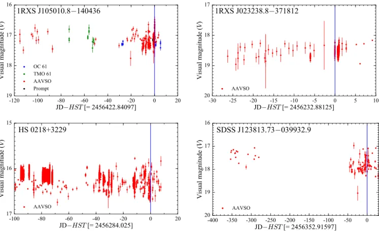
Therefore CVs can easily reach, and exceed, the COS detec-tor safety threshold. The outburst recurrence time ranges from weeks to decades and these events are unpredictable. To avoid damage to the detectors an intensive monitoring of each target was required before the observations. This monitoring program was carried out by the global amateur community and some additional small telescopes (AAVSO, Prompt and many others), and only their outstanding

sup-port has made thisHST survey possible.

Among our 41 COS targets, only

SDSS J154453.60+255348.8 could not be observed since it showed strong variations in its optical brightness in the

days before theHST observation.

After an outburst, the white dwarf does not cool imme-diately to its quiescent temperature since it has been heated by the increased infall of material. The time required to cool back to the quiescent temperature has been modelled and is

related to the outburst amplitude and duration (Sion 1995,

Townsley & Bildsten 2004, Piro et al. 2005). It has been

observed that it can vary from days or weeks up to

sev-eral years (Long et al. 1995,G¨ansicke & Beuermann 1996,

Slevinsky et al. 1999,Piro et al. 2005, seeSzkody et al. 2016

for an extreme case). Therefore the effective temperature measured in a system in which an outburst has recently oc-curred provides only an upper limit for its quiescent effective

temperature and, consequently, forh_M˙_i_.

The right panels of Figure2show three sample COS

ul-traviolet spectra of quiescent CVs in which the white dwarf

dominates the emission, as seen from the broad Lyα

absorp-tion centred on 1216 ˚A. The shape of the Lyαline changes

withTeff, becoming more defined and narrower in the

hot-ter white dwarfs, while the continuum slope of the spectrum becomes steeper.

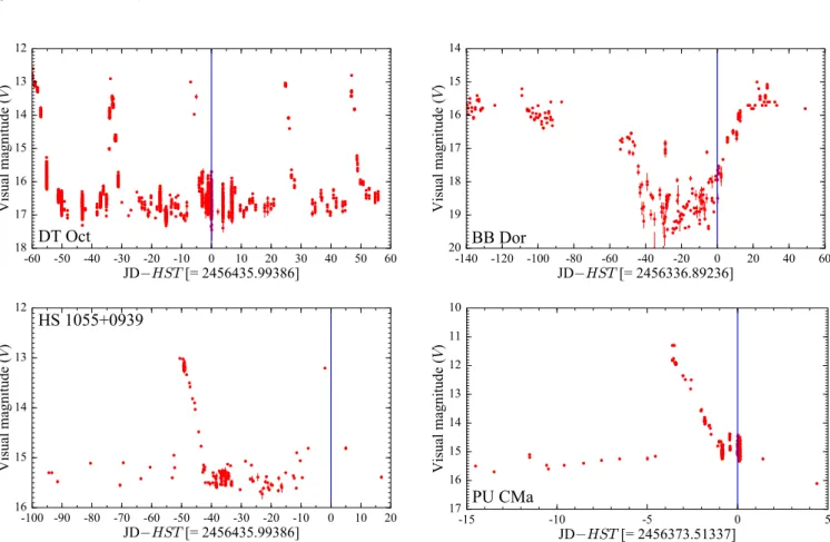
While the majority of the CVs in our sample have

been observed in quiescence (Figure3), obvious signatures

of the white dwarf were missing in the spectra of nine sys-tems: seven of them experienced an outburst shortly before

theHST observation while the remaining two systems are

VY Scl stars (Figure4). This class of CVs is characterised

by high mean accretion rates which keep the disc usually in a stable hot state, equivalent to a dwarf nova in permanent outburst. In this high state, the disc dominates the spec-tral appearance even in the far ultraviolet. However, occa-sionally the accretion rate drops (low state) and unveils the

white dwarf (e.g.G¨ansicke et al. 1999,Knigge et al. 2000,

Hoard et al. 2004). The VY Scl stars in our sample (OR And

and BB Dor) were caught in the high state and intermedi-ate stintermedi-ate respectively, preventing a detection of the white dwarf. For the purpose of completeness, the spectra of these

nine objects are shown in Figure5, but a detailed analysis of

these systems is outside the scope of this paper and will be

presented elsewhere (e.g.Godon et al. 2016). In Section3, we

analyse the 31 systems in which the white dwarf signature

is easily recognisable from a broad Lyαabsorption profile.

2.2 STIS observations

TheSpace Telescope Imaging Spectrograph(STIS) data were collected as part of two snapshot programs (programs ID

9357 and 9724) in Cycle 11 and 12 (Table2). Snapshot

pro-grams are designed to fill short gaps in the weekly HST

observing schedule, therefore each CV was observed with exposure times of only 600 to 900 seconds, through the

52”×0.2” aperture. We used the G140L grating at the

cen-tral wavelength 1425 ˚A and the FUV–MAMA detector to

obtain spectra covering the wavelength range 1150−1700 ˚A

at a nominal resolution ofR ' 1000.

Similar to the COS–FUV detector, the MAMA detec-tor is also subject to damage by excessive illumination but, contrary to the COS program, the snapshot programs did not have a long term schedule which could allow detailed monitoring before the STIS observations. We analysed the STIS acquisition images to determine the source bright-ness immediately before the spectrum acquisition. These

images were acquired with the F28 × 50LP filter

(cen-tral wavelength of 7228.5 ˚A and full width at half–maximum

of 2721.6 ˚A). We determined the corresponding magnitude

following the method described in Araujo-Betancor et al.

(2005b). By comparison with published magnitudes and the

system brightness in the Sloan Digital Sky Survey (SDSS) and AAVSO Photometric All–Sky Survey (APASS), we ver-ified that all the targets were observed in quiescence.

These snapshot programs produced ultraviolet spectra

of 69 CVs (e.g.G¨ansicke et al. 2003,Araujo-Betancor et al.

2005a, Rodr´ıguez-Gil et al. 2004). Here we analyse the

re-maining eight objects in which the white dwarf dominates the ultraviolet emission. We show three sample STIS

spec-tra of quiescent CVs in the left panel of Figure2where the

(5)

Wavelength [Å]

0 2.0 4.0 6.0 8.0

V844 Her

Wavelength [Å]

0 2.0 4.0 6.0 8.0 10.0 12.0

Fλ

[

10

−

15 erg c

m

−

2 s

−

1Å

−

1]

CY UMa

1200 1300 1400 1500 1600 1700

Wavelength [Å]

0 0.5 1.0 1.5

2.0

DV UMa

Wavelength [Å]

0 0.2 0.4 0.6 0.8 1.0

SDSS J103533.02+055158.4

Wavelength [Å]

0 2.0 4.0 6.0 8.0

Fλ

[

10

−

15 erg c

m

−

2 s

−

1Å

−

1]

SDSS J123813.73

−

033932.9

1200 1300 1400 1500 1600 1700

Wavelength [Å]

0 5.0 10.0

15.0

HS 2214+2845

Figure 2.HST/STIS spectra (left) andHST/COS spectra (right) for six objects in which the white dwarf dominates the far–ultraviolet. The geocoronal emission lines of Lyα(1216 ˚A) and Oi(1302 ˚A) are plotted in grey.

-120 -100 -80 -60 -40 -20 0 20

JD

−HST

[= 2456422.84097]

16

17

18

19

Vi

sua

l m

agni

tude

(

V

)

1RXS J105010.8

−

140436

OC 61 TMO 61 AAVSO Prompt

-30 -25 -20 -15 -10 -5 0 5 10

JD

−HST

[= 2456232.88125]

17

18

19

20

Vi

sua

l m

agni

tude

(

V

)

1RXS J023238.8

−

371812

AAVSO

-100 -80 -60 -40 -20 0 20

JD

−HST

[= 2456284.025]

15

16

17

Vi

sua

l m

agni

tude

(

V

)

HS 0218+3229

AAVSO

-400 -350 -300 -250 -200 -150 -100 -50 0

JD

−HST

[= 2456352.91597]

16

17

18

19

20

Vi

sua

l m

agni

tude

(

V

)

SDSS J123813.73

−

039932.9

AAVSO

(6)

Effective Temperatures of CV white dwarfs

5

Table 1.Log of theHST/COS observations. The systems are ordered by orbital period. TheV–band magnitudes listed here are the quiescent values reported from the literature and do not represent the brightness during the COS observations (see Figures3and4).

System Porb Type V E(B−V) Observation Number Total State

(min) (mag) (mag) date of exposure

orbits time (s)

V485 Cen 59.03 SU UMa 17.7 0.071a _{2013 Mar 16} ₄ ₉₉₀₇ _q

GW Lib 76.78 WZ Sge 16.5 0.03b _{2013 May 30} ₃ ₇₄₁₇ _q

SDSS J143544.02+233638.7 78.00 WZ Sge? 18.2 0.029a _{2013 Mar 09} ₃ ₇₁₂₃ _q

OT J213806.6+261957 78.10 WZ Sge 16.1 0.063a _{2013 Jul 25} ₂ ₄₇₆₀ _q

SDSS J013701.06–091234.8 79.71 SU UMa 18.7 0.024c _{2013 Sep 13} ₄ ₁₀₅₀₅ _q

SDSS J123813.73–033932.9 80.52 WZ Sge 17.8 0.006c _{2013 Mar 01} ₃ ₇₁₈₃ _q

PU CMa 81.63 SU UMa 16.2 0.09a _{2013 Mar 22} ₂ ₄₇₅₇ _eq

V1108 Her 81.87 WZ Sge 17.7 0.025c _{2013 Jun 06} ₃ ₇₃₂₇ _q

ASAS J002511+1217.2 82.00 WZ Sge 17.5 0.025c _{2012 Nov 15} ₃ ₇₁₈₃ _q

SDSS J103533.02+055158.4 82.22 WZ Sge? 18.8 0.009c _{2013 Mar 08} ₅ ₁₂₂₈₂ _q

CC Scl 84.10 DN/IP 17.0 0.013a 2013 Jun 29 2 4668 q

SDSS J075507.70+143547.6 84.76 WZ Sge? 18.2 0.028a 2012 Dec 14 3 7183 q

1RXS J105010.8–140431 88.56 WZ Sge 17.0 0.018c 2013 May 10 3 7363 q

MR UMa 91.17 SU UMa 16.7 0.02a _{2013 Apr 04} ₂ ₄₄₀₁ _q

QZ Lib 92.36 WZ Sge 17.5 0.054c _{2013 Apr 26} ₃ ₇₅₁₂ _q

SDSS J153817.35+512338.0 93.11 CV 18.6 0.012a _{2013 May 16} ₂ ₄₇₀₄ _q

1RXS J023238.8–371812 95.04 WZ Sge 18.8 0.027a _{2012 Nov 01} ₅ ₁₂₅₅₆ _q

SDSS J093249.57+472523.0 95.48 DN? 17.9 0.014a _{2013 Jan 11} ₂ ₄₃₂₆ _eq

BB Ari 101.20 SU UMa 17.9 0.105a _{2013 Sep 27} ₂ ₄₈₁₇ _q

DT Oct 104.54 SU UMa 16.5 0.145a _{2013 May 20} ₂ ₄₈₇₅ _eq

IY UMa 106.43 SU UMa 18.4 0.012c _{2013 Mar 30} ₂ ₄₁₉₅ _q

SDSS J100515.38+191107.9 107.60 SU UMa 18.2 0.025a _{2013 Jan 31} ₃ ₇₀₉₃ _q

RZ Leo 110.17 WZ Sge 19.2 0.029c _{2013 Apr 11} ₄ ₁₀₅₀₅ _q

CU Vel 113.04 SU UMa 17.0 <0.02d _{2013 Jan 18} ₂ ₄₆₃₄ _q

AX For 113.04 SU UMa 18.5 0.027c _{2013 Jul 11} ₃ ₇₄₈₃ _q

SDSS J164248.52+134751.4 113.60 DN 18.6 0.063a _{2012 Oct 12} ₃ ₇₂₄₀ _eq

QZ Ser 119.75 SU UMa 17.9 0.038c _{2013 Jun 21} ₄ ₁₀₅₀₅ _q

IR Com 125.34 DN 18.0 0.016c _{2013 Feb 08} ₃ ₆₈₆₆ _q

SDSS J001153.08–064739.2 144.40 U Gem 17.8 0.029a 2012 Nov 09 5 12601 q

OR And 195.70 VY Scl 18.2 0.158a 2013 Jul 10 3 7361 hs

BB Dor 221.90 VY Scl 18.0 0.03a _{2013 Feb 13} ₃ ₇₂₇₂ _is

SDSS J040714.78–064425.1 245.04 U Gem 17.8 0.08a _{2013 Jan 24} ₂ ₄₃₁₅ _q

CW Mon 254.30 U Gem 16.8 0.044c _{2012 Nov 30} ₂ ₄₇₇₄ _eq

V405 Peg 255.81 CV 18.2 0.064c _{2012 Dec 07} ₃ ₇₃₀₃ _eq

HS 2214+2845 258.02 U Gem 16.8 0.078a _{2013 Jun 18} ₂ ₄₆₈₀ _q

BD Pav 258.19 U Gem 15.4 0.0b _{2013 Jun 14} ₃ ₇₃₇₅ _q?

SDSS J100658.41+233724.4 267.71 U Gem 18.3 0.018c _{2014 Mar 20} ₅ ₁₂₄₉₄ _q

HM Leo 268.99 U Gem 17.5 0.021c _{2013 Feb 22} ₄ ₉₉₇₉ _eq

SDSS J154453.60+255348.8 361.84 U Gem? 16.9 0.032c _{2013 Apr 22} _– _– _?

HS 0218+3229 428.02 U Gem 15.5 0.05c _{2012 Dec 22} ₃ ₇₁₅₉ _q

HS 1055+0939 541.88 U Gem 15.5 0.025a _{2013 Apr 15} ₂ ₄₆₈₈ _eq

Notes.TheE(B−V) data have been retrieved from: (a) the NASA/IPAC Extragalactic Database (NED); (b) GW Lib: Bullock et al.(2011), BD Pav:Sion et al.(2008); (c) the three–dimensional map of interstellar dust reddening based on Pan–STARRS 1 and 2MASS photometry (Green et al. 2015); (d) this work. The NED data are the galactic colour excess and represent an upper limit for the actual reddening while the Pan–STARRS data are the actual reddening for the systems with a known distance. The last column reports the state of the system during theHST observations:eq, early quiescence, i.e. observed close to an outburst;q, quiescence;

hs, high state;is, intermediate state.

broad Lyαabsorption centred on 1216 ˚A reveals the white

dwarf photosphere.

Three of the eight systems observed by STIS (BD Pav, QZ Ser and V485 Cen) are in common with the COS sample and we present a detailed comparison of the two datasets in

Section4.2.2.

Adding the five additional CVs observed with STIS to the 31 from the COS survey results in our total sample of 36 CVs in which the white dwarf dominates the overall spectral emission.

3 DATA ANALYSIS

Ultraviolet spectra are particularly suitable for the study of CV white dwarfs because, at these wavelengths, the spectral energy distribution is often dominated by the white dwarf while the donor star does not contribute at all. However, some contamination from the disc, the bright spot (the re-gion where the ballistic stream from the companion inter-sects the disc) or the boundary layer (the interface between the accretion disc and the white dwarf) can dilute the emis-sion from the white dwarf photosphere. As described in

(7)

-60 -50 -40 -30 -20 -10 0 10 20 30 40 50 60

JD

−HST

[= 2456435.99386]

12 13 14 15 16 17 18

Vi

sua

l m

agni

tude

(

V

)

DT Oct

-140 -120 -100 -80 -60 -40 -20 0 20 40 60

JD

−HST

[= 2456336.89236]

14 15 16 17 18 19 20

Vi

sua

l m

agni

tude

(

V

)

BB Dor

-100 -90 -80 -70 -60 -50 -40 -30 -20 -10 0 10 20

JD

−HST

[= 2456435.99386]

12

13

14

15

16

Vi

sua

l m

agni

tude

(

V

)

HS 1055+0939

-15 -10 -5 0 5

JD

−HST

[= 2456373.51337]

10 11 12 13 14 15 16 17

Vi

sua

l m

agni

tude

(

V

)

PU CMa

Figure 4.Sample light curves for four targets in our sample which have been observed close to an outburst or in an intermediate state. The blue line represents the date of the HST observation, which has been subtracted from the Julian date on the x–axis. Note the different time range on the x–axis. The data have been retrieved from the AAVSO database.

Table 2.Log of theHST/STIS observations. The systems are ordered by orbital period. The fourth column reports the instrumental magnitudes measured from the acquisition images, which were obtained through theF28×50LP filter.

System Porb Type F28×50LP E(B−V) Observation Number Total State

(min) (mag) (mag) date of exposure

orbits time (s)

V485 Cen 59.03 SU UMa 17.9 0.071a _{2004 Apr 15} ₁ ₉₀₀ _q

V844 Her 78.69 SU UMa 17.4 0.013c _{2003 Feb 23} ₁ ₉₀₀ _q

UV Per 93.44 SU UMa 17.9 0.0b _{2002 Oct 11} ₁ ₉₀₀ _q

RZ Sge 98.32 SU UMa 18.0 0.302a _{2003 Jun 13} ₁ ₉₀₀ _q

CY UMa 100.18 SU UMa 17.3 0.012a _{2002 Dec 27} ₁ ₈₃₀ _q

QZ Ser 119.75 SU UMa 16.9 0.038c _{2003 Oct 07} ₁ ₉₀₀ _q

DV UMa 123.62 SU UMa 18.6 0.014c _{2004 Feb 08} ₁ ₉₀₀ _q

BD Pav 258.19 U Gem 14.6 0.0b 2003 Feb 09 1 600 q

Notes. TheE(B−V) data have been retrieved from: (a) the NASA/IPAC Extragalactic Database (NED); (b) UV Per:Szkody

(1985), BD Pav: Sion et al. (2008); (c) the three–dimensional map of interstellar dust reddening based on Pan–STARRS 1 and 2MASS photometry (Green et al. 2015). The NED data are the galactic colour excess and represent an upper limit for the actual reddening while the Pan–STARRS data are the actual reddening for the systems with a known distance. The last column reports the state of the system during theHST observations:q, quiescence.

tion2.1, the overall shape of a white dwarf ultraviolet

spec-trum is determined by its effective temperature: hotter white

dwarfs have narrow Lyα profiles and steep blue continua,

while cooler white dwarfs are characterised by broad Lyα

profiles and flat continua. Therefore the white dwarf effec-tive temperature can be accurately measured by fitting the

HST data with synthetic white dwarf atmosphere models.

In Figure6, we show the COS data of 1RXS J023238.8–

371812 as an example of a typical CV spectrum from

our sample. The broad Lyα absorption at ' 1216 ˚A, the

quasi–molecular absorption bands of H+2 at '1400 ˚A and

several sharp absorption lines (e.g. Ci 1460/1490 ˚A, Siii

1526/1533 ˚A, Ci 1657 ˚A) reveal the white dwarf

photo-sphere. The white dwarf dominates the ultraviolet

emis-sion but the non–zero flux detected in the core of the Lyα

(8)

Effective Temperatures of CV white dwarfs

7

0 0.5 1.0 1.5 2.0 2.5

BB Dor

0 1.0 2.0 3.0 4.0

5.0

CW Mon

1200 1300 1400 1500 1600 1700

0 2.0 4.0

6.0

DT Oct

1200 1300 1400 1500 1600 1700

0 0.5 1.0 1.5 2.0

2.5

HM Leo

1200 1300 1400 1500 1600 1700

0 0.5 1.0 1.5 2.0

Fλ

[

10

−

14

erg c

m

−

2

s

−

1Å

−

1

]

HS 1055+0939

1200 1300 1400 1500 1600 1700

0 0.1 0.2 0.3

0.4

OR And

1200 1300 1400 1500 1600 1700

0 4.0 8.0 12.0 16.0

18.0

_{PU CMa}

1200 1300 1400 1500 1600 1700

0 1.0 2.0

3.0

SDSS J093249.57+472523.0

1200 1300 1400 1500 1600 1700

Wavelength [

Å

]

0 4.0 8.0

12.0

V405 Peg

Figure 5.HST/COS spectra of the nine CVs dominated by emis-sion from the accretion flow, outshining the white dwarf. Strong emission lines of Ciii(1175 ˚A), Nv(1242 ˚A), Cii(1335 ˚A), Siiv

(1400 ˚A), Civ(1550 ˚A) and Heii(1640 ˚A) are clearly visible. The wavelength ranges affected by the geocoronal emission lines of Lyα(1216 ˚A) and Oi(1302 ˚A) are plotted in grey.

a hot boundary layer, or from the disc (Long et al. 1993,

Godon et al. 2004,G¨ansicke et al. 2005). In addition we

de-tect emission lines, which are broadened by the Keplerian velocity distribution of the disc. A model to fit the data has to account for these three contributions (white dwarf, second component and emission lines) detected in a CV spectrum.

We usedtlusty andsynspec(Hubeny 1988;Hubeny

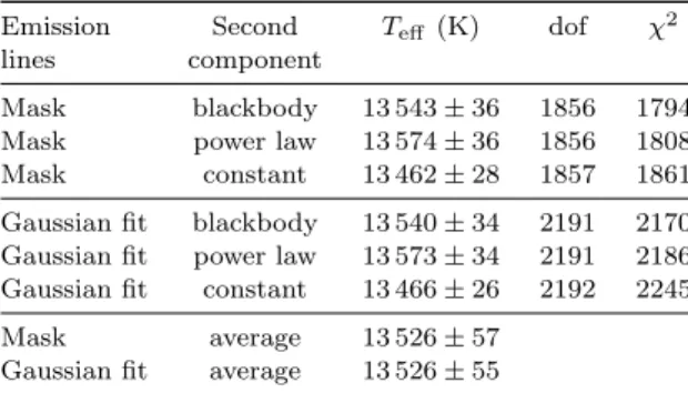
Table 3.Results for 1RXS J023238.8–371812 for the two different fitting methods for the disc emission lines, in which we either mask the emission lines (Mask) or include them as Gaussian profiles (Gaussian fit). We fixed logg= 8.35. The last two rows (average) report the mean and the standard deviations for each method.

Emission Second Teff (K) dof χ2

lines component

Mask blackbody 13 543±36 1856 1794

Mask power law 13 574±36 1856 1808

Mask constant 13 462±28 1857 1861

Gaussian fit blackbody 13 540±34 2191 2170 Gaussian fit power law 13 573±34 2191 2186 Gaussian fit constant 13 466±26 2192 2245

Mask average 13 526±57

Gaussian fit average 13 526±55

& Lanz 1995) to compute a grid of synthetic spectra of white

dwarf atmospheres, coveringTeff = 10 000−70 000 K in steps

of 100 K, and metal abundancesZ of 0.01, 0.10, 0.20, 0.50

and 1.00 times their solar values2_.

Ideally, a spectral fit to the ultraviolet data would

pro-vide bothTeffand the surface gravity (logg). However these

two quantities correlate: an increase in the temperature translates into a larger fraction of ionised hydrogen and nar-rower Lyman and Balmer lines; this effect can be counter-balanced by a higher gravity which increases pressure broad-ening. It is not possible to break this degeneracy from the

sole analysis of theHST data since they only provide the

Lyαabsorption profile which, in the case of cool CV white

dwarfs, is limited to only the red wing of the line. Therefore we needed to make an assumption on the surface gravity. Most previously published work analysing CV white dwarf

ultraviolet spectra assumed logg = 8.00, corresponding to

0.6 M, the average mass of isolated white dwarfs (Koester

et al. 1979,Liebert et al. 2005,Kepler et al. 2007), unless an

independent white dwarf mass determination was available.

However,Zorotovic et al.(2011) demonstrated that the

av-erage mass of white dwarfs in CVs is actually higher than

that of isolated white dwarfs,'0.8 M(logg'8.35). Since

the canonical assumption logg = 8.00 does not reflect the

observed average mass of CV white dwarfs, we generated

our grid of models assuming logg= 8.35.

The COS ultraviolet spectra are contaminated by

geo-coronal emission of Lyαand Oi1302 ˚A, and we masked these

wavelength regions for our spectral analysis. Furthermore, we noticed the presence of an additional continuum

compo-nent in all our systems, which contributes'10−30 per cent

of the observed flux. In order to account for this, we included

in the fit a blackbody, a power law or a constant flux3 (in

2 _{Using a single metallicity is sufficient to account for the}

pres-ence of the metal lines in the fit, which are relatively weak. Pos-sible deviations of single element abundances from the overall scaling with respect to the solar values do not affect the results of theχ2 _{minimisation routine. In fact, varying the abundances}

of individual elements has no effect on the measuredTeff. 3 _{The constant is a special case of a power law and accounts for}

the easiest case with no slope, as it requires only one free param-eter (a scaling factor), while power law and blackbody require two (respectively, a temperature and an exponent, plus a

(9)

H

+₂

C

iii

N

v

C

ii

Si

iv

C

i

C

i

C

i

_Si

_ii

C

iv

He

ii

Wavelength [˚

A]

F

λ

[1

0

−

1

5

er

g

cm

−

2

s

−

1

˚ A

−

1

]

1200 1300 1400 1500 1600 1700

2.0

1.5

1.0

0.5

0

Figure 6.HST/COS spectrum of 1RXS J023238.8–371812. Plotted in green are the emission lines of Ciii(1175 ˚A), Nv(1242 ˚A), Cii

(1335 ˚A), Siiv(1400 ˚A), Civ(1550 ˚A) and Heii(1640 ˚A). The red band underlines the position of the H+₂ quasi–molecular absorption bands. The blue band highlights the presence of a second, flat continuum component which, in this case, contributes'10 per cent of the observed flux. The geocoronal emission lines of Lyα(1216 ˚A) and Oi(1302 ˚A) are plotted in grey.

Fλ), which can reproduce different slopes in the second

com-ponent and are representative of different physical processes (thermalised emission in the case of the blackbody, optically

thin emission in the case of the power law). Using aχ2

min-imisation routine, we fitted the grid of model spectra to the

HST data and measured the effective temperatures of the

36 CV white dwarfs.

To investigate the influence of the disc emission lines on our fitting procedure, we carried out our spectral analysis using two different methods: (i) we masked all the emission

lines (Mask); (ii) we included the emission lines as Gaussian

profiles, allowing three free parameters: amplitude,

wave-length and width (Gaussian fit).

We illustrate the differences between the two

meth-ods using 1RXS J023238.8–371812. Figure7shows the COS

spectrum along with the best–fit models obtained masking the emission lines (left panels) and including the lines in the fit (right panels), for all three different second components (from top to bottom: blackbody, power law and constant). The temperatures measured with the two methods typically

only differ by' 3 K (see Table3), demonstrating that

in-cluding or masking the disc lines has no influence on the

fit result (see alsoSzkody et al. 2010). Therefore, to use as

much of the data as possible, we decided to include the lines

in the fit (Gaussian fit).

The uncertainties of the individual fits listed in Table3

are purely statistical, as derived from the fitting procedure. They are unrealistically small and do not reflect the real uncertainties, which are instead dominated by several sys-tematic effects, analysed in the following sections.

ing factor). For this reason, we included the constant flux as an additional mode for the second component.

3.1 The unknown nature of the second component

The first systematic uncertainty in our fitting procedure arises from the unknown nature of the additional emission component. The blackbody, the power law or the constant are not constrained outside the ultraviolet wavelength range, and only serve to account for different slopes in the de-tected additional continuum component. They thus repre-sent a very simplified model of the additional continuum contribution and it is likely that none of them provides a realistic physical description of this emission component.

From a statistical point of view, and owing to the lim-ited wavelength coverage of our data, we cannot discriminate among the three of them, and they all result in fits of sim-ilar quality and in very simsim-ilar temperatures for the white

dwarf (see Table 3). These differences in Teff reflect a

sys-tematic effect related to presence of this additional flux. For

this reason, we decided to adopt as finalTeff measurement

the mean of the results obtained with the three different additional components. To evaluate the magnitude of the related systematic uncertainty, we calculated both the

stan-dard deviation of the Teff values obtained with the three

different additional components and the sum in quadrature of the statistical errors of the individual fits. We assumed as final and more realistic estimate for the systematic uncer-tainty the larger of these two. Additional systematic effects are analysed in the following sections.

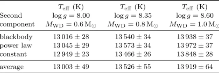
3.2 The unknown white dwarf mass

As pointed out above, the temperature and mass of a white

dwarf correlate. Table4reports the effective temperatures of

1RXS J023238.8–371812 allowing different logg(= different

white dwarf masses). These results show that an

assump-tion on loggtranslates into an accurate measurement of the

temperaturefor a given mass('50 K), while the systematic

(10)

1200 1300 1400 1500 1600 1700

Wavelength [

Å

]

0 0.5 1.0 1.5 2.0

F

λ

[

10

−

15

erg c

m

−

2

s

−

1

Å

−

1

]

T =

13543 ± 36

K

BB

1200 1300 1400 1500 1600 1700

Wavelength [

Å

]

-20 2

Re

sidua

ls

₁₂₀₀ ₁₃₀₀ ₁₄₀₀ ₁₅₀₀ ₁₆₀₀ ₁₇₀₀

Wavelength [

Å

]

0 0.5 1.0 1.5

F

λ

[

10

−

15

erg c

m

−

2

s

−

1

Å

−

1

]

T =

13540 ± 34

K

BB

1200 1300 1400 1500 1600 1700

Wavelength [

Å

]

-20 2

Re

sidua

ls

1200 1300 1400 1500 1600 1700

Wavelength [

Å

]

0 0.5 1.0 1.5 2.0

F

λ

[

10

−

15

erg c

m

−

2

s

−

1

Å

−

1

]

T =

13574 ± 36

K

PL

1200 1300 1400 1500 1600 1700

Wavelength [

Å

]

-20 2

Re

sidua

ls

₁₂₀₀ ₁₃₀₀ ₁₄₀₀ ₁₅₀₀ ₁₆₀₀ ₁₇₀₀

Wavelength [

Å

]

0 0.5 1.0 1.5 2.0

F

λ

[

10

−

15

erg c

m

−

2

s

−

1

Å

−

1

]

T =

13573 ± 34

K

PL

1200 1300 1400 1500 1600 1700

Wavelength [

Å

]

-20 2

Re

sidua

ls

1200 1300 1400 1500 1600 1700

Wavelength [

Å

]

0 0.5 1.0 1.5 2.0

F

λ

[

10

−

15

erg c

m

−

2

s

−

1

Å

−

1

]

T =

13462 ± 28

K

const

1200 1300 1400 1500 1600 1700

Wavelength [

Å

]

-20 2

Re

sidua

ls

₁₂₀₀ ₁₃₀₀ ₁₄₀₀ ₁₅₀₀ ₁₆₀₀ ₁₇₀₀

Wavelength [

Å

]

0 0.5 1.0 1.5 2.0

F

λ

[

10

−

15

erg c

m

−

2

s

−

1

Å

−

1

]

T =

13466 ± 26

K

const

1200 1300 1400 1500 1600 1700

Wavelength [

Å

]

-20 2

Re

sidua

ls

(11)

10000.0 20000.0 30000.0 40000.0 50000.0

log (T

8. 35

[K])

−4000 −3000 −2000 −1000 0 1000 2000 3000 4000

∆

T

eff

[K

]

DW UMa

Z = 0.71 Z⊙

DW UMa

Z = 0.71 Z⊙

∆

+

_T

eff

= T

eff

(log g = 8. 60) − T

eff

(log g = 8. 35)

∆

−

_T

eff

= T

eff

(log g = 8. 00) − T

eff

(log g = 8. 35)

Figure 8. Best–fit to ∆+_T

eff = Teff(logg = 8.60)−Teff(logg = 8.35) and ∆−Teff =Teff(logg = 8.00)−Teff(logg = 8.35), as a

function ofTeff(logg= 8.35), for the five metallicities and the three additional continuum second components (red for blackbody, blue

for power law and gold for constant). The fit excludes the effective temperatures of (i) the eclipsing systems IY UMa, SDSS J040714.78– 064425.1 and SDSS J100658.41+233724.4 for which disc absorption along the line of sight makes the identification of the continuum flux level difficult (Section4.4); (ii) CC Scl and SDSS J164248.52+134751.4 for which a reliable effective temperature determination was not possible (Section4.2); (iii) SDSS J153817.35+512338.0 because the core of its narrow Lyαline is strongly contaminated by geocoronal airglow emission which makes the data less sensitive to a change in the model surface gravity. DW UMa was not included in the fit, but serves as independent test of the fit.

Table 4.Tefffor 1RXS J023238.8–371812 allowing different logg,

corresponding to different white dwarf masses. These results have been obtained fitting the data including the emission lines as Gaussian profiles, and using three different models for the sec-ond component.

Teff (K) Teff (K) Teff (K)

Second logg= 8.00 logg= 8.35 logg= 8.60 component MWD= 0.6 M MWD= 0.8 M MWD= 1.0 M

blackbody 13 016±28 13 540±34 13 938±37 power law 13 045±29 13 573±34 13 972±37 constant 12 949±23 13 466±26 13 848±28

average 13 003±49 13 526±55 13 919±64

is typically an order of magnitude larger ('500 K).

There-fore the dominant source of error is the (unknown) white dwarf mass and we used the following approach to evaluate

how this systematic uncertainty depends onTeff.

As shown byZorotovic et al.(2011), the average mass

of CV white dwarfs is 0.83±0.23M and we therefore

investigated the correlation between effective temperature

and logg in the mass range 0.6 M(logg = 8.00) to

1.0 M(logg = 8.60). We fitted our HST data assuming

logg = 8.00, logg = 8.35 and logg = 8.60 for each

metallicity and for each type of second component, resulting

in 15 effective temperatures (five metallicities×three

sec-ond components) for each logg, for each object. We define4

as T8.00 = Teff(logg = 8.00), T8.35 = Teff(logg = 8.35)

and T8.60 = Teff(logg = 8.60), and calculated ∆+Teff =

T8.00−T8.35, and ∆−Teff =T8.60−T8.35.

We excluded from this analysis the eclipsing

systems IY UMa, SDSS J040714.78–064425.1 and

SDSS J100658.41+233724.4 for which disc absorption

along the line of sight makes the identification of the

continuum flux level difficult (Section4.4). We also did not

include CC Scl and SDSS J164248.52+134751.4 for which a reliable effective temperature determination was not

possi-ble (Section 4.2), and SDSS J153817.35+512338.0 because

the core of its narrow Lyα line is strongly contaminated

by geocoronal airglow emission which makes the data less sensitive to a change in the model surface gravity.

The remaining objects have typicallyTeff . 21 000 K,

with the exception of HS2214+2845 (Teff ' 26 000 K).

To better constrain ∆+_T

eff and ∆−Teff and to verify the

validity of this relationship at high temperatures, we in-cluded in our analysis two additional hotter objects: SS Aur

(Teff = 34 000±2 000 K for logg = 8.8, Sion et al. 2008)

and DW UMa (Teff = 50 000±1 000 K for logg= 8.00 and

Z = 0.71 Z,Araujo-Betancor et al. 2003). Both these

ob-jects have been observed with STIS, which allows the

re-4 _{We found that the effective temperature derived for different}

(12)

Effective Temperatures of CV white dwarfs

11

moval of the contamination from geocoronal emission and therefore, differently from SDSS1538 in our sample, they can be used to constrain the relationship at high temperatures. We retrieved the STIS spectrum of SS Aur and the out–

of–eclipse STIS low–state spectrum of DW UMa (Knigge

et al. 2000) from theHST data archive. Following the same

method as for the CVs in our sample, we fitted these data

assuming logg = 8.00, logg = 8.35 and logg = 8.60. For

SS Aur we found: T8.00 = 26 269±275 K,T8.35 = 27 507±

282 K andT8.60= 28 402±270 K forZ= 0.1 Z. In the case

of DW UMa, we assumedZ = 0.71 Z, and obtainedT8.00=

49 900±844 K, in agreement with Araujo-Betancor et al.

(2003), T8.35 = 52 532±893 K and T8.60= 54 282±986 K,

respectively.

Figure 8 show the trend of ∆+Teff and ∆−Teff as a

function ofTeff(logg= 8.35). These correlations are well fit

with the following relation:

∆Teff =alog(Teffb) (1)

wherea= 1054(2) K,b= 0.0001052(7) K−1_{for ∆}+_T

eff, and

a=−1417(2) K,b= 0.0001046(5) K−1 for ∆−Teff.

We included the SS Aur temperatures in the fit of

∆+Teff and ∆−Teff to better constrain the relationship

at high temperatures. In contrast, we did not include the DW UMa temperatures and we only overplot them in

Fig-ure8to illustrate that our best–fit is in good agreement with

this independent measurement.

The two best–fit curves represent the systematic

un-certaintyσTeff due to the unknown mass of the white dwarf.

The two curves are not symmetric (since the relationship

be-tween loggand the white dwarf mass is not linear), resulting

in asymmetric error bars with ∆−Teff >∆+Teff. However,

to simplify our discussion, we adopted as final uncertainty

the larger value derived from ∆−Teff:

σTeff = 1417 log(0.0001046Teff) (2)

In summary, we found that the systematic uncertainty due to the unknown white dwarf mass lies in the range

300−1800 K. Once the masses for each system are accurately

determined, the degeneracy between Teff and logg will be

broken, reducing the uncertainties in Teff to those related

to the unknown nature of the second additional component

(see Section3.1).

3.3 Reddening

Reddening due to interstellar dust along the line of sight can introduce an additional systematic uncertainty in the effective temperature determination as it affects the overall slope of the ultraviolet spectra. However, CVs are intrinsi-cally faint and thus we are observationally biased towards nearby systems, for which extinction is usually negligible. Moreover, owing to their colour similarity with quasars, CVs are often discovered by extragalactic surveys (such as SDSS), which cover high Galactic latitudes, and are therefore not heavily affected by reddening. To verify that reddening is a minor contribution to the total error budget, for all the systems in our sample, we compiled the colour excess of

our CVs (Table1and 2) using the three–dimensional map

of interstellar dust reddening based on Pan–STARRS 1 and

0.00 0.05 0.10 0.15 0.20 0.25 0.30 0.35

E(B − V) 13800

13900 14000 14100 14200 14300 14400 14500 14600

Teff

Figure 9.Best–fit effective temperatures for UV Per, obtained by reddening theHST/STIS data for increasing values ofE(B−V). The blue lines show the systematic uncertainties on the effective temperature derived from the fit to the original data (E(B−V) = 0), following the method described in Section3.1. They establish the threshold above which the effect of interstellar absorption on ourTeff is greater than the systematic uncertainties, i.e.E(B−

V)'0.1.

2MASS photometry (Green et al. 2015) wherever possible,

i.e. when the distance is known and the object is inside the field covered by this map. For the remaining objects, we re-port either the value from the literature where available or

the galacticE(B−V) from the NASA/IPAC Extragalactic

Database (NED), which only represents an upper limit for the actual reddening. Finally, for CU Vel, we determined its

colour excess below (Section4.3.1.1).

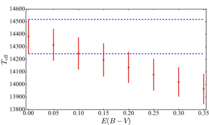
To establish how the interstellar absorption affects our analysis, we considered one of the systems with zero colour excess, UV Per, and reddened its spectrum using the

rela-tionship given byCardelli et al.(1989) for a range of values

inE(B−V). Since we previously determined the effective

temperature for this CV white dwarf,Teff[E(B−V) = 0] =

14 389±578 K, we can use this “artificially reddened” dataset

to study the variation of Teff as a function of reddening.

We fitted the reddened spectra following the prescription

from Sections3and3.1and show the derived temperatures

in Figure9. The interstellar absorption introduces a

vari-ation in Teff greater than the systematic uncertainties

de-fined in Section3.1(blue dashed lines) forE(B−V)&0.1,

which we assumed as the threshold above which the effect of the reddening cannot be neglected. Only one system in our sample has a colour excess significantly higher than this

value: RZ Sge,E(B−V) = 0.302, as returned from the NED

database. However Sagittarius lies on the Galactic plane and

thisE(B−V) represents an estimate over the entire

Galac-tic column. Given the typical distances of CVs, the actual reddening of RZ Sge is likely to be lower than that. We

as-sumed the mass–radius relationship fromVerbunt &

Rap-paport(1988) and, using the scaling factors from the fit to

the STIS data for different surface gravities (Section 3.2),

we estimated the distance to RZ Sge to lie in the range

262 pc . d . 335 pc, for 0.6 M ≤ MWD ≤ 0.8 M.

From the three–dimensional map of interstellar dust

redden-ing (Green et al. 2015) we found 0.044 . E(B−V) .0.070,

well below the threshold we established above. We therefore considered negligible the reddening for this system.

Finally, interstellar gas along the line of sight can also

contaminate the observed spectrum with additional Lyα

(13)

drogen column density and reddening fromDiplas & Savage

(1994), we determined that this contribution is always of the

order of few ˚Angstrom ('3 ˚A for E(B−V) = 0.05 up to

' 7 ˚A for E(B−V) = 0.3) and therefore much narrower

than the white dwarf Lyα absorption line. In fact, the

in-terstellar Lyα absorption is located in the spectral region

that we always masked owing to geocoronal airglow

emis-sion, which typically has a width of '18 ˚A, and therefore

we concluded that interstellar Lyαabsorption has no effect

on our results.

3.4 Other possible systematic effects

To review all the systematic uncertainties in a way as com-prehensive as possible, we need to discuss the possibility of

Lyαabsorption from the additional non–white dwarf

com-ponent and inaccuracies in the instrument calibration. Although not much is known about the physical origin of the second component, it is likely to arise from a hot op-tically thick (e.g. the bright spot) or a hot opop-tically thin medium surrounding a cooler optically thick layer (e.g. the disc or the boundary layer). It is therefore possible that the second component can contribute, to some extent, to the

observed Lyαabsorption. The Lyαprofile is, along with the

spectral slope, the main tracer of the white dwarf tempera-ture, and such a hypothetical contamination could

system-atically affect our results.Long et al.(2009) investigated an

additional Lyβ absorption in VW Hyi finding that it most

likely originates from a hot spot region whose emission can

be approximated by a stellar model with logg ' 4. The

Lyman absorption lines arising from such an environment are consequently significantly narrower than the white dwarf

Lyαabsorption itself, which is broadened by the higher

pres-sure on the white dwarf surface at logg '8.35. Thus,

al-though the model we used to describe the additional com-ponent does not account for the possibility of absorption in

the Lyαregion, such contamination (if present) would not

appreciably affect our effective temperature determination. Finally, limitations in the instrument calibration may

affect our results. Massa et al.(2014) report that the

sys-tematic uncertainties in the COS G140L flux calibration are

less than two per cent forλ <1200 ˚A and one per cent for

1200 ˚A< λ <1900 ˚A, with an increase up to six per cent at

λ= 2150 ˚A. Owing to a decrease in the detector sensitivity

in the red portion of the spectrum, we only considered the

wavelength range 1150 ˚A< λ <1730 ˚A, for which systematic

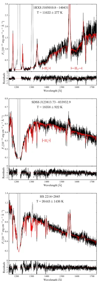
uncertainties are less than two per cent. The maximum ef-fect on our results can be evaluated by multiplying the COS spectra with a linear function with a two per cent slope. To assess also for possible dependencies with the tempera-ture of the white dwarf, we choose three systems representa-tive of cool, warm and hot white dwarfs: 1RXS J105010.8– 140431, SDSS J123813.73–033932.9 and HS 2214+2845. We fitted their spectra after applying the two per cent slope in

flux calibration and find that the resultingTeff values are in

agreement, within the uncertainties, with the one we derived from the original COS data. We therefore conclude that our analysis is not affected by the very small uncertainty in the COS instrument calibration.

Three objects in our sample have been observed both

with STIS and COS. In Section4.2.2 we compare the two

1200 1300 1400 1500 1600 1700

0 0.5 1.0 1.5 2.0 2.5

Fλ

[

10

−

15 erg c

m

−

2 s

−

1Å

−

1]

H+

2 H2

T = 11622 ± 277 K

1200 1300 1400 1500 1600 1700

Wavelength [Å] -2

-10

1 2

Re

sidua

ls

1200 1300 1400 1500 1600 1700

0 0.1 0.2 0.3 0.4 0.5 0.6 0.7 0.8

Fλ

[

10

−

14 erg c

m

−

2 s

−

1Å

−

1]

H+

2

SDSS J123813.73−033932.9

T = 18358 ± 922 K

1200 1300 1400 1500 1600 1700

Wavelength [Å] −2

−10

1 2

Re

sidua

ls

1200 1300 1400 1500 1600 1700

0 0.2 0.4 0.6 0.8 1.0 1.2 1.4

Fλ

[

10

−

14 erg c

m

−

2 s

−

1Å

−

1]

HS 2214+2845 T = 26443 ± 1436 K

1200 1300 1400 1500 1600 1700

Wavelength [Å] -2

-10

1 2

Re

sidua

ls

Figure 10.Ultraviolet spectra (black) of cool, warm and hot CV white dwarfs in our sample along with the best–fit model (red) assuming a blackbody second component. The quasi–molecular absorption bands of H+₂ and of H2 are visible at'1400 ˚A and

'1600 ˚A forTeff . 19 000 K andTeff .13 500 K, respectively

(14)

emis-Effective Temperatures of CV white dwarfs

13

datasets and, for this comparison to be reliable, we needed to verify that the STIS and COS calibrations agree. To do

so, we retrieved from theHST archive the STIS and COS

data of the flux standard WD 0308–565. We overplot the one available STIS spectrum and the COS data acquired at different epochs, finding that the STIS spectrum matches the flux level of all the COS data. With a linear fit to the ratio between the two datasets, we determined that they

differ, on average, by'3 per cent. This comparison proves

that uncertainties in the STIS calibration are comparable to the systematic uncertainties of COS and therefore they are negligible in our analysis. Finally, we can also conclude that the differences in the STIS and COS effective temperatures

discussed in Sections 4.2.2 are not related to calibration

issues of the two instruments.

We followed the procedure outlined in the previous

Sec-tions to fit theHST data of the 36 CVs and summarize the

results in Table5. Figure10shows three examples of best–

fit models obtained with this procedure: 1RXS J105010.8– 140431 (top panel), SDSS J123813.73–033932.9 (middle panel) and HS 2214+2845 (bottom panel), which are rep-resentative of different temperature regimes (cool, interme-diate and hot, respectively). All the spectra, along with their best–fit models, are available in the online material.

4 DISCUSSION

4.1 loggcorrection of publishedTeff values

The two most commonly used techniques to measure effec-tive temperatures of CV white dwarfs are spectroscopy, that is by fitting ultraviolet or optical spectra with white dwarf atmosphere models, and photometry, i.e. from the analysis of light curves to study the white dwarf ingress and egress

in eclipsing systems. Townsley & G¨ansicke(2009, hereafter

TG09) present an analysis of CV white dwarf effective tem-peratures and selected only those systems for which a

re-liableTeff determination is available. They consider a

mea-surement unreliable when obtained from (i) spectra in which the white dwarf could not be unambiguously detected or, (ii) in the case of eclipse light curve analyses, oversimplified models or data of poor quality were used. Following these criteria, TG09 compiled 43 systems with a reliable temper-ature measurement (see their table 1).

Among the 43 measurements from TG09, 15 were ob-tained from light curve analyses (which also delivers the white dwarf mass) or have a white dwarf mass measurements independent from the spectral fit. For the remaining 28 ob-jects an independent mass determination was not available

and the white dwarf Teff was evaluated via spectroscopic

analyses, following methods similar to the one described

here, but assuming logg= 8.00. As discussed in Section3,

this assumption does not reflect the average mass in CV

white dwarfs,M '0.8 M, corresponding to logg= 8.35.

To combine our results with those of TG09, we need

there-fore to evaluate the correspondingTeff for logg= 8.35 for

those 28 objects.

The systematic correction that we need to apply is

∆Teff = Teff(logg = 8.35)−Teff(logg = 8.00), which is

the opposite of the quantity ∆−Teff we calculated in

Sec-tion3.2. Using the relationship−∆−Teff = 1417×log(Teff×

0.0001046), we corrected the Teff values for those 28

sys-tems from TG09 which did not have an independent mass measurement to the average CV white dwarf mass (i.e.

logg= 8.35), therefore enabling a consistent combinations

of these values with the 36 temperatures that we derived for the COS+STIS data.

4.2 Notes on individual objects

4.2.1 Systems observed close to an outburst

As explained in Section2, if a CV experienced an outburst

shortly before the ultraviolet observation, its spectrum could be contaminated by disc emission. Furthermore the white dwarf photosphere is heated by the increased infall of ma-terial and different subtypes of CVs have different cooling time scales on which they return to their quiescent

temper-ature (Sion 1995,Piro et al. 2005). A spectroscopic analysis

of these systems can therefore provide only an upper limit on the white dwarf effective temperature.

For each system, we inspected the light curves re-trieved from the AAVSO web site plus a total of

addi-tional ∼ 2000 images (collected with the Mount John

University Observatory OC61 Telescope, the New Mex-ico State University Observatory TMO61 telescope and the Prompt telescopes located in Chile), covering two

months before theHST/COS observations. We found that

nine systems in which the white dwarf dominates the ul-traviolet flux went into outburst within this time inter-val: AX For, BB Ari, HS 2214+2845, IY UMa, MR UMa,

QZ Ser, V485 Cen (Figure11), CC Scl (Figure12, left), and

SDSS J164248.52+134751.4 (SDSS1642, Figure 12, right).

QZ Ser and V485 Cen have STIS observations (Section4.2.2)

from which we determined the quiescent temperature while, for the remaining systems, the results that we report here

only represent an upper limit for their quiescentTeff.

For CC Scl and SDSS1642, we found that the white

dwarf contributes only'35 per cent (Figure13, top) and

'50 per cent of the total flux (Figure13, bottom),

respec-tively. Owing to this strong disc contamination, the derived effective temperatures do not fulfil the requirement of a re-liable measurement as defined in TG09, and we do not in-clude them in the following analysis. Furthermore CC Scl is an Intermediate Polar (IP) and its response to accretion and disc instabilities is more complicated than that of a non– magnetic CV. This system will be analysed in more detail by Szkody et al. (2016, in preparation).

4.2.2 Systems with COS and STIS observations

QZ Ser and V485 Cen have been observed both with COS

and STIS (Table6). Inspecting their spectra (middle and

bottom panel of Figure 14), the COS observations have a

higher flux compared to the STIS observations, which is also reflected in their effective temperatures; the STIS data

re-turn a lower value (QZ Ser:Teff = 14 481±587 K, V485 Cen:

Teff = 15 200±655 K) compared to the COS data (QZ Ser:

Teff = 15 425±676 K, V485 Cen:Teff = 16 208±746 K). This

difference is not related to difference in the calibration of the

two instruments (see Section3.4) and it is rather expected

given that the magnitudes derived from the STIS acquisi-tion images suggest that these systems were observed by

(15)

System Porb d MWD References Z Teff ± WD Instrument

(min) (pc) (M) (Z) (K) (K) contribution

V485 Cen 59.03 1 0.5 15 200 655 56% STIS

GW Lib 76.78 140+30₋₂₀ 2, 3 0.2 16 995↓ 812 85% COS

SDSS J143544.02+233638.7 78.00 4 0.01 11 940 315 84% COS

OT J213806.6+261957 78.10 5 0.2 16 292 753 69% COS

V844 Her 78.69 290±30 3, 6 0.1 14 850 622 61% STIS

SDSS J013701.06–091234.8 79.71 300±80 7, 8 0.1 14 547 594 77% COS

SDSS J123813.73–033932.9 80.52 110 9 0.5 18 358 922 75% COS

PU CMa 81.63 10 COS

V1108 Her 81.87 130±30 11, 12 1.0 13 643 503 81% COS

ASAS J002511+1217.2 82.00 130±30 12, 13 0.1 12 830 416 77% COS

SDSS J103533.02+055158.4 82.22 170±12 0.835±0.009 14, 15 0.01 11 620 44* 85% COS

CC Scl 84.10 16 0.2 16 855: 801 35% COS

SDSS J075507.70+143547.6 84.76 17 0.5 15 862 716 90% COS

1RXS J105010.8–140431 88.56 100±50 18, 19 0.1 11 622 277 89% COS

MR UMa 91.17 20 0.2 15 182↓ 654 69% COS

QZ Lib 92.36 120±50 19 0.01 11 303 238 64% COS

SDSS J153817.35+512338.0 93.11 17 0.01 33 855 1785 94% COS

UV Per 93.44 21 0.2 14 389 578 75% STIS

1RXS J023238.8–371812 95.04 160 22 0.2 13 527 491 78% COS

SDSS J093249.57+472523.0 95.48 17 COS

RZ Sge 98.32 20 0.5 15 287 663 56% STIS

CY UMa 100.18 23 0.1 15 232 658 61% STIS

BB Ari 101.20 24, 25 0.2 14 948↓ 632 83% COS

DT Oct 104.54 24, 25 COS

IY UMa 106.43 190±60 0.79±0.04 26, 27 1.0 17 750↓ 1000* 77% COS

SDSS J100515.38+191107.9 107.60 17 0.2 15 944 723 74% COS

RZ Leo 110.17 340±110 28, 29 0.5 15 014 638 83% COS

CU Vel 113.04 150±50 29, 30 0.1 15 336 668 89% COS

AX For 113.04 370+20−60 25, 31 1.0 16 571↓ 777 68% COS

SDSS J164248.52+134751.4 113.60 32 1.0 17 710: 871 48% COS

QZ Ser 119.75 460+150₋₁₁₀ 33 0.2 14 481 587 68% STIS

DV UMa 123.62 504±30 1.098±0.024 15, 34 1.0 18 874 182* 92% STIS

IR Com 125.34 300 22, 35 1.0 16 618 781 86% COS

SDSS J001153.08–064739.2 144.40 36 0.1 13 854 525 63% COS

OR And 195.70 25 COS

BB Dor 221.90 1500±500 37 COS

SDSS J040714.78–064425.1 245.04 38 1.0 20 885 1104 67% COS

CW Mon 254.30 297 25, 39 COS

V405 Peg 255.81 149+26−20 40 COS

HS 2214+2845 258.02 41 0.5 26 443↓ 1436 84% COS

BD Pav 258.19 500 42, 43 0.5 17 775 876 92% STIS

SDSS J100658.41+233724.4 267.71 676±40 0.78±0.12 44 1.0 16 000 1000* 96% COS

HM Leo 268.99 350 45 COS

HS 0218+3229 428.02 1000 46 0.2 17 990 893 70% COS

HS 1055+0939 541.88 25 COS

Notes.For each object, its orbital period, distance and white dwarf mass are compiled from the literature. The last columns report the results from this work: metallicity, effective temperatures, the systematic uncertainties arising from the unknown white dwarf mass, the percentage of the white dwarf contribution to the total flux and the instrument used. The white dwarf contribution has been calculated assuming a constant flux as second component. For the four systems highlighted with a star, a precise mass measurement is available. While the uncertainties on the effective temperature of IY UMa and SDSS1006 are dominated by the presence of the curtain of veiling gas (Section4.4), the uncertainties reported for SDSS1035 and DV UMa are those related the unknown nature of the second additional component (Section3.1). In particular, for DV UMa, we report the effective temperature obtained assuming log g = 8.78 (Section4.3.2). The values flanked by a downwards arrow represent upper limits for the temperature of the systems. The values flanked by a colon represent unreliable effective temperature and are not considered in the discussion.

References.(1)Augusteijn et al.(1996), (2)Thorstensen(2003), (3)Thorstensen et al.(2002a) (4)Szkody et al.(2007), (5)Chochol et al.(2012), (6)Oizumi et al.(2007), (7)Pretorius et al.(2004), (8)Imada et al.(2007), (9)Aviles et al.(2010), (10)Thorstensen & Fenton(2003), (11)Price et al.(2004), (12)Ishioka et al.(2007), (13)Templeton et al.(2006), (14)Littlefair et al.(2006), (15)Savoury et al.(2011) (16)Chen et al.(2001), (17)G¨ansicke et al.(2009), (18)Mennickent et al.(2001), (19)Patterson et al.(2005a), (20)

Patterson et al.(2005b), (21)Thorstensen & Taylor(1997), (22)Patterson(2011), (23)Thorstensen et al.(1996), (24)Uemura et al.

(2010), (25)Ritter & Kolb(2003), (26)Steeghs et al.(2003), (27)Patterson et al.(2000), (28)Mennickent & Tappert(2001), (29)