5558.pdf

(1)

POPULATION-AVERAGED MODELS FOR

DIAGNOSTIC ACCURACY STUDIES AND

META-ANALYSIS

James Murray Powers

A dissertation submitted to the faculty of the University of North Carolina at Chapel Hill in partial fulﬁllment of the requirements for the degree of Doctor of Philosophy in the Department of Biostatistics.

Chapel Hill 2013

Approved by:

(2)

c ⃝ 2013

(3)

Abstract

JAMES MURRAY POWERS: Population-averaged models for diagnostic accuracy studies and meta-analysis

(Under the direction of Dr. John S. Preisser and Dr. Haitao Chu)

(4)

outcomes is estimated with GEE in the meta-analysis of two data sets. It is com-pared to an indirect method of estimation of PA parameters based on transformations of bivariate random effects model parameters. The third paper presents an analysis guide for a new SAS macro, PAMETA (Population-averaged meta-analysis), for fit-ting population-averaged (PA) diagnostic accuracy models with GEE as described in the second paper. The impact of covariates, influential clusters and observations is investigated in the analysis of two example data sets.

(5)

(6)

Acknowledgments

The road traveled during this program has been a long one. Through the years there have been some people who have supported me unconditionally during this time. First, John Preisser and I have been working together since the beginning of my program, early on as my GRA advisor and eventually my dissertation co-advisor. John has always been supportive of my program progress and dissertation, provided excellent advice when I sought guidance, delivered constructive criticism when needed and always found time to help me with anything I needed.

To my best friend and partner for life, Kimberly, thanks for your patience during the particularly diﬃcult times during this process.

I would also like to thank Quintiles, where I have worked for many years of this doctoral program. Quintiles provided ﬁnancial support to me (and hundreds of other working students) over the years. In addition, Quintiles allowed for ﬂexible work sched-ules when needed in order to pursue academic interests.

There are far too many people to list here who have helped me in various ways over the years. I provide here a ﬁnal general acknowledgement to each person whom I have had the pleasure of working with has provided me with a key insight or skill that has allowed me to continue through this process.

(7)

List of Tables

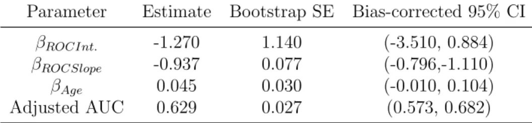
2.1 Results of linear model for DPOAE in control subjects only, estimated with GEE to account for clustering of ears within subjects . . . 49 2.2 Results of ROC-GLM model, case subjects standardized to controls, all

data . . . 50 2.3 Change in AUC with removal of inﬂuential subjects . . . 51

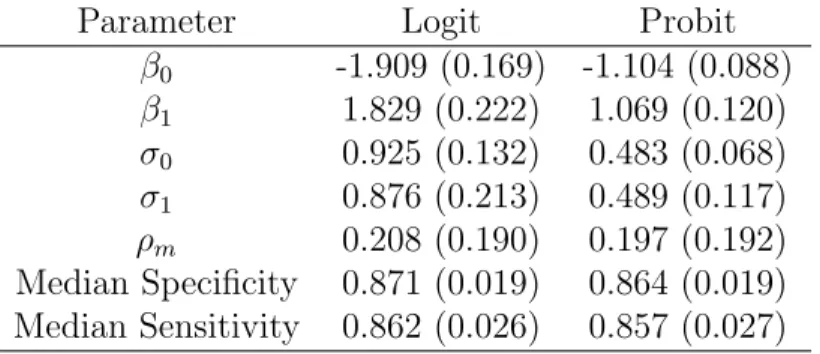
3.1 Comparison of PA Logit and Probit models with heterogeneous scale for clusters for the catheter segment culture data , as well as the GLMM-converted analogs. All standard errors reported are empirical except for PA parameters ϕ0, ϕ1 andρg which are estimated via a 2-stage bootstrap

approach. . . 71 3.2 Results of GLMM model for Logit and Probit links for the catheter

segment culture data (from Chu et. al (2010)) . . . 72 3.3 Simulated Data: Comparison of Logit and Probit link functions for the

PA method heterogeneous scale for clusters. All standard errors reported are empirical except for PA parametersϕ0, ϕ1andρg which are estimated

via a 2-stage bootstrap approach. . . 73 3.4 Simulated Data: Results of GLMM model for Logit and Probit links . . 74 3.5 Percent coverage of nominal 95% conﬁdence intervals based upon

empir-ical standard errors after ﬁtting PA model as well as SS-model marginal converted results . . . 75

4.1 Data from a Meta-Analysis of Studies on Semi-Quantitative (Type=1) or Quantitative (Type=2) Catheter Segment Culture for Diagnosis of Intravascular Device-Related Bloodstream Infection. (Source: Chu et al. (2010) . . . 95

(11)

4.2 Comparison of Full and Reduced models for the catheter segment culture data (all data), for PA model with logit link (bias-corrected standard errors) . . . 96 4.3 Studies 18 and 20 removed: Comparison of Full and Reduced models for

the catheter segment culture data (all data),for PA model with logit link (bias-corrected standard errors) . . . 97 4.4 Data from a Meta-Analysis of Studies on lymph node metastases. (Source:

Klerkx et al. (2010) . . . 98 4.5 Comparison of Full and Reduced models for the lymph node metastases

data (all data), for PA model with logit link (bias-corrected standard errors) . . . 99 4.6 Study 28 removed: Comparison of Full and Reduced models for the

(12)

List of Figures

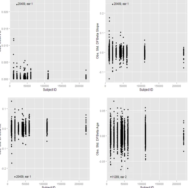
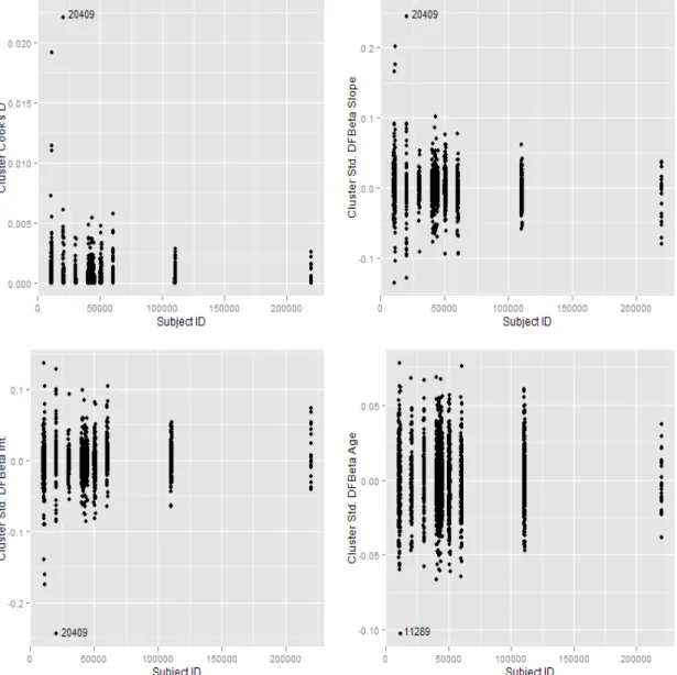
2.1 Observation deletion diagnostics for Control Reference Distribution lin-ear model portion of ROC-GLM. . . 45 2.2 Cluster deletion diagnostics for Control Reference Distribution linear

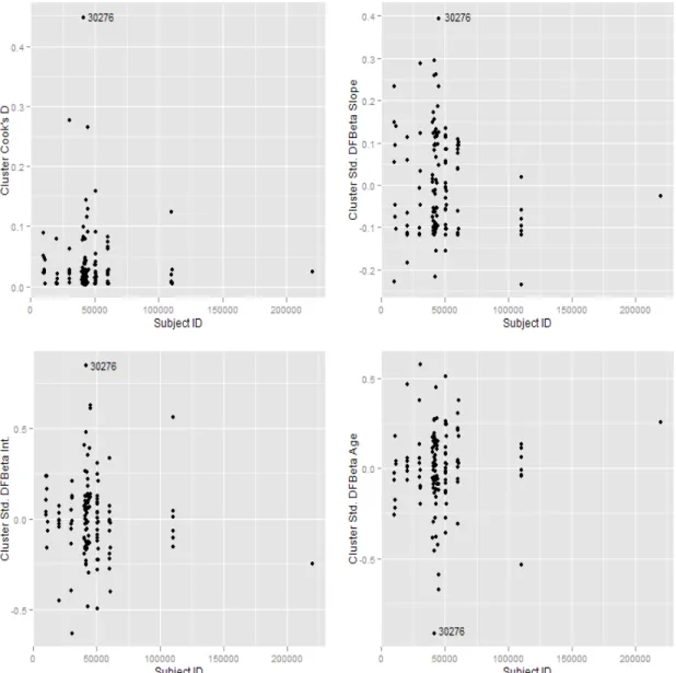
model portion of ROC-GLM. DFBETAs are standardized by use of em-pirical standard errors. . . 46 2.3 Covariate adjusted ROC curves for Age (age=50 top line, age=40 middle

line, age=30 lower line) for both full model (solid curves) and model without subjects 20409 and 11289 (dashed lines) . . . 47 2.4 Cluster deletion diagnostics for ROC regression portion of ROC-GLM. 48

3.1 GLMM prediction region and PA model mean estimate with 95% conﬁ-dence region. Upper left: Chu et al. 2010 data, logit link; Upper right: Chu et al. 2010 data, probit link; Lower left: Expanded and balanced data, logit link; Lower right: Expanded and balanced data, probit link. The conﬁdence region is the smaller area contained within the prediction region. . . 70

4.1 Deletion diagnostics for catheter segment culture data. Upper left panel: Cluster (Study) level Cook’s D; upper right: Observation (sensitivity and 1- speciﬁcity within a cluster) Cook’s D; lower left: DFBETAS for 1-speciﬁcity; and, lower right: DFBETAS for sensitivity. . . 93 4.2 Deletion diagnostics for lymph node metastases data. Upper left panel:

Cluster (Study) level Cook’s D; upper right: Observation (sensitivity and 1- speciﬁcity within a cluster) Cook’s D; lower left: DFBETAS for 1-speciﬁcity; and, lower right: DFBETAS for sensitivity. . . 94

(13)

Chapter 1 Literature Review

1.1 Introduction to Diagnostic Test Accuracy

Modern medical decision making often involves one or more diagnostic tools (such as laboratory tests and/or radiographic images). These diagnostic tools are developed us-ing the most current technology available, and are often welcomed into medical practice with the hope of improving the care for patients. A diagnostic tool must be evaluated for it’s discriminatory ability to detect presence (or absence) of current health state. The basic properties of quantitative evaluation of diagnostic tools were set forth over half a century ago in the ﬁeld of signal detection. The quantitative properties of a decision tool involve assessments of how well the tool discriminates between states.

Using the notation of Pepe (2003), the variable for true disease status is deﬁned as

D= 1 for a diseased subject and D= 0 for a non-diseased subject. The notation of ¯D

for non-diseased andD for diseased subjects is also frequently used when displaying equations for the regression models. The variableY is the result of the diagnostic test: Y = 1 indicates positive disease status, while Y = 0 denotes negative disease status.The measures of accuracy displayed next include the disease-speciﬁc

(14)

(T P F). T P F is also referred to as sensitivity, while 1−F P F is also known as specificity. The first measures of accuracy of interest are those of quantifying the misclassification probabilities for each disease group. The ideal test would have no false positives or false negatives, since these are considered errors. The true and false positive fractions are defined as:

F P F =P[Y = 1|D= 0]

T P F =P[Y = 1|D= 1]

These quantities address the question: to what degree does the test reﬂect the true disease state? The ideal test hasF P F = 0 andT P F = 1, while a completely

uninformative test has T P F =F P F. The F P F and T P F can be considered either probabilities or fractions. However, these are often called false positive and true positive ‘rates’, which they are not (Pepe, 2003) because the numerator and

denominator are in the same scale. There is a large body of literature concerning the analysis of binary tests, most of which is based upon the theory of 2x2 tables. Speciﬁc topics for binary tests including methods for a single test, multiple tests and

regression models are summarized in Pepe (2003).

1.2 Introduction to ROC Curves

While it is natural to think of diagnostic tests in terms of a dichotomous outcome, in practice many tests are created on a continuous or ordinal scale and then possibly simpliﬁed into a dichotomous outcome (such as a pregnancy test). The previous section introduced measures of diagnostic accuracy and possible analysis models, all assuming the test of interest was dichotomous. Diagnostic tests that are measured on a continuous or ordinal scale are now examined.The consideration must be made that

(15)

since there are more than just two possible outcomes of the test, there is now more than just one 2x2 table to consider. For each result of a given test, there is an associated set of accuracy measures. The Receiver Operating Characteristic (ROC) curve is a device that describes the range of tradeoﬀs between failing to detect disease and falsely identifying disease with the test (Pepe, 2003).

The development of the ROC curve can be traced back to the early 1950s where it was developed for signal detection and radar applications (Metz, 1986). In the 1950s, the ﬁrst application of ROC to a medical test was completed when researchers

attempted to quantify the ability of a Pap smear analyzer to discriminate between malignant and benign tissue samples (Zweig and Campbell, 1993). In the 1960s, ROC plots began to surface in psychology and psychophysics studies (Metz, 1986). Lusted (1960) provided the first paper on using “logical analysis” in radiology by presenting decision making tradeoffs with an ROC curve. The statistical development of ROC analysis can be traced initially to Patton (1978) who gives the first decidedly

statistical summary presenting the probability theory in the context of a 2x2 decision analysis. Dorfman and Alf (1968) presented a maximum likelihood method that was used in early binormal ROC curve analysis, but this was not presented speciﬁcally as an ROC-speciﬁc method at the time.

(16)

1.2.1 Notation and Properties

Pepe (2003) summarized the attributes of ROC curves for evaluating diagnostic tests as providing a complete description of test performance, facilitating comparing and combining information across studies of the same test, guiding the choice of threshold value and providing a mechanism for relevant comparisons between diﬀerent

non-binary tests. Since the ROC curve transforms all results to the T P F and F P F

scale, comparisons of diﬀerent tests can be examined for the same disease, regardless of the units or scale of measurement.

The ROC curve can be viewed as a function that describes the distance between distributions. While the focus is typically on diagnostic tests, it is possible to use an ROC curve as an exploratory curve any time interest lies in the diﬀerence between the distribution of two groups. Brumback et al. (2006) provided an interpretation for the ROC curve when used to describe the diﬀerences between two treatment groups in a clinical trial, for example. By using a threshold , it is possible to transform a

continuous test result into a dichotomous outcome. Assuming a test, Y , is positive if

Y ≥cand negative if Y < c then the following represent the responses of controls and cases, respectively,

Y_Dj¯ , j = 1, . . . , n_D¯

YDi, i= 1, . . . , nD

It is assumed that Y_Di¯ and YDi are randomly selected from the population of test

results associated with the diseased and non-diseased states (Pepe, 2003).

(17)

The deﬁnition of T P F and F P F may then be augmented:

T P F(c) = P[Y ≥c|D= 1]

F P F(c) = P[Y ≥c|D= 0]

The ROC curve is then deﬁned as the entire set of T P Fand F P F pairs after dichotomizingY with diﬀerent values ofc:

ROC(·) = [(F P F(c), T P F(c)), c∈(−∞,∞)]. (1.1)

When c=∞, then limc→∞T P F(c) = 0 and limc→∞F P F(c) = 0, while at the

opposite end of the interval we have c=−∞, then limc→−∞T P F(c) = 1 and

limc→−∞F P F(c) = 1. It is also possible to write the ROC curve as

ROC(·) = [(t, ROC(t)), t∈(0,1)] (1.2)

wheret =F P F(c) and ROC(t) = T P F(c) =T P F(F P F−1(c)).

The ROC curve is a monotone increasing function mapping two [0,1] intervals. The uninformative test has an ROC curve that has unit slope through the unit square. In this case the distributions of test results for the diseased and non-diseased subjects are identical. On the other end of the spectrum the perfect test has an ROC curve that traces the left and upper limits of the unit square sinceT P F(c) = 1 andF P F(c) = 0.

1.2.2 ROC Estimation Methods

Empirical Method

(18)

area under the curve) and are not smooth (resembling a Kaplan-Meier type of shape). Zweig and Campbell (1993) argued that continuous diagnostic tests should employ the purely nonparametric method since parametric methods were developed for ratings data. Hsieh and Turnbull (1996) later deﬁned the asymptotic properties of the empirical ROC curve. The empirical ROC curve is a function only of the ranks of the data because it only depends on the relative orderings of the test results and their diseased status. For each possible cut-point c, the empirical estimates of T P F and

F P F are, respectively:

[

T P F(c) =

nD

∑

i=1

I[YDi ≥c]/nD (1.3)

[

F P F(c) =

n_D

∑

i=1

I[Y_Dj ≥c]/n_D (1.4) The empirical ROC curve is a plot of T P F[(c) versus F P F[(c) for all c∈(−∞,∞) and denoted by ROC[e(t). This is considered a discrete function because F P F[(c) can

only take on values in increments of 1/ n_D. Joining these points on a graph gives a step function with vertical jumps of 1/ nD corresponding to subjects from diseased

subjects, while horizontal jumps of 1/ n_D are made from subjects in the non-diseased group. Ties within each group result in larger vertical or horizontal jumps, while ties in test results between diseased and non-diseased subjects result in diagonal jumps. A confidence band for the ROC curve was presented in Hsieh and Turnbull (1996). The topic of nonparametric confidence bands for the ROC curve is identified as an area requiring more statistical research (Pepe, 2003).

The empirical area under the curve is the Mann-Whitney U-statistic:

[

AU Ce = n_D ∑ j=1 nD ∑ i=1 (

I[YDi > YDj] +

1

2I[YDi =YDj]

)

/nDnD. (1.5)

(19)

When there are no ties between diseased and non-diseased observations the above expression simpliﬁes to:

[

AU Ce = nD

∑

j=1

nD

∑

i=1

(

I[YDi > YDj]

)

/nDnD. (1.6)

Hanley and McNeil (1982) presented results for the asymptotic variance when observations are independent. DeLong et al. (1988) discussed an alternative representation of the asymptotic variance. The variability of theAU C is often calculated using the bootstrap, especially when the data are clustered (Pepe, 2003). In the case of clustered data, such as when a subject contributes multiple test data, bootstrap resampling is performed at the cluster level.

Examples of other nonparametric methods include Zou et al. (1997) and Zhou et al. (2002) who presented studies in kernel density smoothing. They both use kernels and bandwidth selection procedures, however they arrive at the smooth curve in a slightly diﬀerent way. Their work provides some interesting theoretical results to help

determine the theoretical basis and justiﬁcation for smoothing in ROC curve analysis.

Parametric Method

With its foundation in Gaussian distribution theory, the binormal curve has become a common analysis tool for ROC curves, most commonly in the radiology imaging evaluation area. Metz (1986) and Metz et al. (1998) are just two of dozens of articles written by Charles Metz and colleagues. Despite being motivated based on

Gaussian-distributed test results, later it will become evident that this condition may be relaxed. GivenYD ∼N(µD, σ2D) and YD* ∼N(µD, σ2D) then the ROC curve is

deﬁned as

(20)

wherea = µD−µD

σD ,b=

σ_D

σD and Φ is the standard normal cumulative distribution function. Using the convention that larger test results are more indicative of disease

a >0, sinceµD > µD. The binormal method produces smooth curves which are

aesthetically pleasing. Also, the binormal model is appealing for ordinal predictors as is often found in radiology studies for example (Metz et al., 1998).

1.3 Covariate Adjustment of ROC Curves

When considering binary tests it was observed that regression models could be ﬁt for

F P Fand T P F separately, as well as predictive values and DLRs. Methods have been developed to ﬁt models to continuous data, which are analogues to those ﬁt to

F P Fand T P F. Covariate eﬀects are evaluated on the non-disease reference

distribution and the ROC curve which quantiﬁes the discriminatory capacity of the test (Pepe, 2003).

Evaluation of covariate eﬀects on the non-disease reference distribution FX

determines which factors affect the false positive fractions when a test threshold is fixed. Stated another way, it is determined whether thresholds should be defined differently for sub-populations with different covariate values in order to keep F P F

constant across these subgroups. The methods for this are straightforward, making use of regression quantiles. When covariate eﬀects are modeled on the ROC curve itself, the issue of interest is whether or not the covariates aﬀect the ability of the test to discriminate disease from non-disease independent of threshold (Pepe, 2003).

Inference about the accuracy of a given test may be biased if covariate eﬀects are neglected (Pepe, 2003). The classic case of confounding occurs when test results are related to covariates and the distributions of the covariates are diﬀerent for both the diseased and non-diseased populations (Pepe, 2003). However, it is also possible to have bias when the distributions are the same in both populations. There are two

(21)

cases to consider: the covariate aﬀects only the test result, or the covariate aﬀects the ROC curve but not the test results. The radiology literature has much discussion on attenuation of the ROC curve by ignoring covariates on the distribution of the test results (Rutter and Gatsonis, 2001). In the case of radiology studies, the

’reader-speciﬁc’ ROC curve attenuates the overall ROC curve due to diﬀering usage of the rating scale for a given image.

When deciding whether to present the pooled or covariate-speciﬁc curves,

consideration should be given to what use the test result will have. If the test result and given threshold will be used for a given covariate level (such as age group), then the covariate-speciﬁc curve is of practical importance. However, if the test were to be used across all age groups then the pooled curve is more relevant. For the second case, where the covariate does not aﬀect the test results of the non-diseased

population but does aﬀect the ROC curve, the pooled ROC curve can be thought of as a weighted average of the covariate-speciﬁc ROC curves. In this case the covariate level ROC curves are of interest. Pepe (2003) observed that in data analysis

situations it may be useful to present both the pooled and covariate-speciﬁc curves.

1.3.1 Indirect Regression Methods

The ﬁrst method for evaluating covariate eﬀects on ROC curves was proposed by Tosteson and Begg (1988) and would later be followed up by Toledano and Gatsonis (1995). Although these two papers considered primarily ordinal data, the concepts apply more generally (Pepe, 1998).

For continuous data the approach of this method is to modelFX for both cases and

(22)

that describe the covariate eﬀects of test results. In this case the parameters quantify covariate eﬀects on the ROC curve. Note that the discrete ROC function framework is adopted for this model as opposed to the latent variable posture. The reason for this is that standard statistical packages do not handle the estimation properly due to the dependence of the scale parameter on disease and status and covariates.

It is possible to ﬁt a location-scale model without specifying FX, which is then a

semi-parametric alternative to the previous methods listed above. In this case, quasi-likelihood may be used for estimation of the parameters. The induced curve ROC estimate does require an estimator for FX. A proposed estimate is found in

Pepe (1998), which estimates FX with the empirical distribution of the standardized

residuals which is very similar to a semi-parametric regression quantile estimator. Location-scale models that incorporate random effects are often fit to acknowledge the correlations between test results. In the context of diagnostic accuracy evaluation, fitting these random effects models is no different than other applications (Pepe, 2003). Random effects models can also provide insight into test result variability. In the radiology setting multiple readers of a set of images present a level of correlation that may be important to quantify using random effects. The random effects

formulation of the location-scale models presented previously would be of interest when there are a large number of readers and inference is to be generalized to the entire population of readers. Gatsonis (1995) followed by Ishwaran and Gatsonis (2000) presented advanced discussion of this topic. Etzioni et al. (1999) proposed a random eﬀects model for longitudinal data regarding PSA testing. Finally, both Gonen and Heller (2010) and Devlin et al. (2010) have proposed models that are considered to be Lehmann Family models.

In summary, the indirect models assume a functional form of the distribution of the test results. This can impose unnecessary restrictions on the modeling process.

(23)

This prompted a new avenue of research into methods with less assumptions about the distributional form of the test results.

1.3.2 Direct Regression Methods

The ﬁrst direct regression method was proposed by Pepe (1997) using ordinal data and applying the GEE for estimation. The individual test results are transformed to indicators that are then used for modeling. Using the notation of Pepe (2003), the variable for true disease status is deﬁned as Di = 1 for a diseased subject and Di = 0

for a non-diseased subject. The notation of ¯D for non-diseased and D for diseased subjects is used when displaying equations for the regression models. The variableYi

is the diagnostic test result for subject i. Let {Y_D¯_j, j = 1, ... , n_D¯} and

{YDi, i= 1, ... , nD} represent the ordinal or continuous responses of controls and cases, respectively, with larger values being more indicative of disease. It is assumed that YDi and YD¯i are randomly selected from the population of test results associated with the diseased and non-diseased states (Pepe, 2003). Next, we define a covariate vector,X, which contains the covariates that affect the test result distribution in control subjects, as well as those that affect the discrimination between cases and controls. Finally, we define a set oft discrete points f =f1, ... , ft, on the x-axis of

the ROC curve, chosen from the interval (0,1), over which the model will be ﬁt. For these points, deﬁne

Uit=I[Yi ≥FD−,X1j(t)]−g(α(t), βX) (1.8)

(24)

test results to create binary indicators as the response variable in the GLM:

Uij =I(YDi ≥YDj¯ ) (1.9)

There are two components to the ROC-GLM regression model. The ﬁrst is the vector of covariate valuesX and the second is the speciﬁcation of the ROC curve as a

function of f. If h0(·) and g0(·) are monotone increasing (or decreasing) functions on (0,1) then

g(ROCX(f)) =h0(f) +βX (1.10) is an ROC-GLM regression model (Pepe, 2000).

Further work on the ROC-GLM occurred in Alonzo and Pepe (2002) and Pepe (2000). The concept of estimating a reference distribution for the control subjects and then standardizing case test results to these as “percentile” values are the basis of creating the model. We summarize, and then expand upon, the following 3 general steps required to perform a covariate adjustment of ROC curves using the ROC-GLM (Janes et al., 2009):

1. Estimate P VDXi =FX(YDXi), the percentile values of the test results for cases, whereFX is the distribution of test results in controls as a function of the

covariates.

2. Estimate the cdf of the percentile values as a function of the covariates.

3. Specify the adjustment of the ROC curve as a function of the covariates. We then employ GEE for binary data to estimate the model parameters (covered in Section 2.2).

First, an estimate of FX, the distribution of test results in the control group, is

required. Essentially, we begin the process of standardizing the test results by ﬁnding

(25)

the baseline relationship among the controls. A simple linear model could be speciﬁed (Janes et al., 2009) such that

Y_D¯_i =ψ0+ψ

′

1Xi+ϵi. (1.11)

whereϵi are i.i.d.as N(0, σ2).

We observe that this is the ﬁrst opportunity to apply ordinary linear model deletion diagnostics (such as Cook’s D for simple linear models) in the estimation steps of the ROC-GLM. Given that the model in (2.1) is crucial to the remaining steps, it is proposed that deletion diagnostics be applied at this step to assess the control distribution model. We present the deletion diagnostics in a following section.

Having settled on a linear model in the previous step, and having assumed Gaussian errors for this linear model, then the percentile values for the cases are deﬁned as

d

P VDXi = Φ

(

(YDXi−ψˆ0− ˆ

ψ′₁Xi)/σˆ

)

. (1.12)

If Gaussian errors and/or a linear relationship are too restrictive for a given

application, there are other alternatives proposed. For example, Heagerty and Pepe (1999) propose an empirical estimation of the error distribution using the residuals of the linear model. Further, instead of assuming a linear relationship of the test result in the controls, one could use a stratiﬁed approach (Janes et al., 2009).

At this stage we have now standardized the test results for the cases as a function of the controls by the above step. Next, we must estimate the cdf of the percentile values.

(26)

write:

hX(f) = ROCX(f) = P(1−P VDX ≤f) = g(β0+β1g−1(f)) (1.13) whereg(·) gives a parametric form of the ROC curve; g = Φ is the standard normal c.d.f. andg(·) = exp(·)/[1 +exp(·)] is the logistic function giving binormal and bilogistic ROC curves respectively.

The result after this second step is an ROC curve that is not yet adjusted for covariates that discriminate between the cases and controls. However we do now have an ROC curve that is inherently adjusted for how covariates aﬀect the test

distribution results. This is quite important as Pepe (2003) demonstrates that ”pooled” or unadjusted ROC curves are biased.

The final step in the model specification is to create the inputs for a regression model using the newly created percentile value cdf, and the covariates that are assumed to affect the discriminatory capacity of the test. In other words, covariates that affect the intercept and/or slope of the ROC curve. Recall that we have defined

T discrete points on the x-axis of the ROC curve over which to fit the model. We also defineUit =I1−P V_DXi≤ft, t = 1, ..., T, as the set of cumulative binary indicators which determine whether or not the percentile values are less than each choice of f. For example, if we chose t= 10 values of f then each subject would have a vector of 10 binary indicators for each percentile value within a cluster. Next, we define the covariates XDg−1(f) as those that will enter the model as ones that affect

discrimination. The complete model combining steps 2 and 3 is:

ROCX,XD(f) = g(β0+β1g −1

(f) +β₂′XD+β

′

3XDg−1(f)) (1.14)

We may think of this ﬁnal step as deﬁning a model that has as its output a“baseline” ROC curve (from step 2 and in equation 2.3) and some additional model parameters

(27)

that specify covariate-adjustments of that baseline curve. The previous steps also allow for flexibility in defining which covariates are important for adjusting the control test results distribution and those which affect the discrimination between cases and controls. At this point it is important to note that Pepe (2003) advocate using bootstrap standard errors for the estimates ˆβ from the fitted model. The reason is that since we do not have true independence between responses and covariates there could be bias in the standard errors. In the case of a covariate that affects both the test result distribution and the discriminatory capacity, this covariate would essentially influence both the responses Uit and the covariates in X.

Pepe (2003) suggested using the independence working covariance matrix for ﬁtting the model. Any method for estimating the reference distribution (regression quantiles) may be used, though the empirical method is most robust (Pepe, 2003). The choice of fis important since this will determine the interval over which the model is to hold. The number of points inf, (denoted earlier as ft) should be ﬁnite

so that standard statistical software can handle the estimation. There is currently no method designed to choose the values in the domain that give optimally eﬃcient results (Pepe, 2003). Alonzo and Pepe (2002) found relatively good eﬃciency for small values of ft. Pepe (2003) suggests that in practice it is possible to estimate

parameters with increasing the number of points in ft, stopping when the decreases in

standard errors become small.

Estimation of the ROC-GLM model proceeds following the generalized estimating equations (GEE) procedure (see Chapter 2 for details). Recall from above that hX(f)

deﬁnes the basis for the ROC curve (having standardized cases to the control

(28)

hX(f) is not formally parameterized (Cai and Pepe, 2002). Other research in this

area include Cai and Moskowitz (2004) who proposed a proﬁle MLE of ROC with binormal basis function (a special case of ROC-GLM with no covariates), as well as a pseudo-MLE (where covariates can be included). Pepe and Cai (2004) developed an extension of Cai and Pepe (2002) where semi-parametric ROC-GLM can be viewed as a transformation model of the placement values. In practice, assuming a probit or logistic basis function for the ROC curve is a reasonable assumption which eliminates the need for computation of methods such as Pepe and Cai (2004).

1.3.3 ROC Regression Model Diagnostics

Cai and Zheng (2007) introduced model checking diagnostics for the ROC-GLM. The asymptotic distributions are derived for cumulative residual-based model diagnostics for ROC regression models. The proposed method is an extension of model diagnostic procedures for traditional GLM models originally presented in Lin et al. (2002). The ROC-GLM extension of three model checks (adequacy of ROC-GLM model, link function and interaction of covariate eﬀects with FPF) is based upon the

semi-parametric ROC-GLM presented in Cai and Pepe (2002). Given the task of simultaneously evaluating the test result distributions as well as the relationship between them requires these important extensions. One practical application of this could be investigating the linearity of time in a longitudinal study. It is possible to test whether time enters the model linearly and adjust the coeﬃcients by perhaps adding a quadratic term to the model.

It is natural to ask whether data from a single case (subject) has a large inﬂuence relative to other cases on the estimates in the marginal mean model. For the h-th element of β,interest is often in ( ˆβh−βˆh[i]),the diﬀerence in the parameter estimate with and without thei-th case included in the data. Preisser and Qaqish (1996)

(29)

introduced computationally quick approximations for both observation- and cluster-deletion diagnostics for GEE. However, only the latter, which we call case-deletion, are relevant for this application because the observation-level diagnostics have no real interpretation in the ROC-GLM. Recall that the

Uit, t = 1, . . . , ni, are a set of binary placement value indicators constructed for the

i-th case in the course of applying the estimation method; they don’t have any inherent meaning as individual data values.

Following the formulae of Hammill and Preisser (2006), the inﬂuence of the i-th case as given by the p×1 vector ( ˆβ1−βˆ1[i], . . . ,βˆp −βˆp[i]) can be approximated any further iterations following convergence of the GEE iteratively weighted least squares algorithm by

DF BET ACi =M−1D′iV−

1

i (I−Hi)−1ri

whereHi =DiM−1D′iV−

1

i is the cluster leverage matrix. Note that DF BET ACi is a

measure of the inﬂuence that each cluster has on the estimate of each parameter element of β.Further, there is a close relationship of the set of

DF BET ACi, i= 1, . . . , K with the bias-corrected variance estimator

Vbc(βb) = K

∑

i=1

(DF BET ACi)(DF BET ACi)′

Standardization of DF BET ACi is achieved by dividing each of its elements by the

standard error of its respective parameter estimate, usually based on the full data. Finally, a measure of the inﬂuence of the i-th cluster on the overall model ﬁt can be estimated by Cook’s D:

(30)

where var( ˆβ) is estimated by either the empirical (as in Ziegler et al. (1998) and Preisser et al. (2012)) or bias-corrected variance estimators deﬁned above. Additional details are provided in Chapters 2 and 4.

1.4 Meta-analysis of Diagnostic Tests

Evidence-based decisions in health care are becoming increasingly utilized. From pharmaceutical development programs to medical treatment regimens in practice, the heightened awareness of methods to analyze data in support of health care decisions requires quantitative methods for summarizing the evidence. Meta-analysis, decision analysis and cost-eﬀectiveness analysis are the cornerstones of evidence-based

medicine (Petitti, 2000). The meta-analysis of diagnostic tests is of particular interest in certain screening programs for certain diseases such as cancer. Cervical cancer screening in women and prostate cancer screening in men are both examples of heath screening programs that have a great deal of diagnostic test accuracy studies to draw from for meta-analysis.

Meta-analysis of clinical trials may be employed using various methods that attempt to find the mean effect, however for diagnostic studies the typical summary data points are two dimensional . These measures tend to be positively correlated since studies tend to vary in how test positivity is defined (Pepe, 2003). In the

paragraphs below the evolution of the statistical methods for diagnostic test accuracy meta-analysis are presented. Pepe (2003) lists three beneﬁts of meta-analysis for diagnostic tests: awareness within the research community of previous studies, explanation of discrepancies between individual study results and identiﬁcation of common mistakes in study design thereby providing guidance for design of future studies. For the interested reader, two excellent books reviewing the broad spectrum of general meta-analysis considerations and statistical methods include Hedges and

(31)

Olkin (1985) and Petitti (2000).

1.4.1 The Summary ROC curve

Moses et al. (1993) propose a summary ROC curve for the set of values ofT P F and

F P F, which we denote as (T P Fk, F P Fk) for each of k studies summarized in the

meta-analysis. The ROC-like curve, called sROC, is a curve that goes through the scatter plot of each T P F and F P F pair. In contrast to standard ROC analysis the resultant curve need not yield a monotonic curve (Walter, 2002).The regression equation proposed is D=a+bS where

D=log(T P F/1−T P F)−log(F P F/1−F P F) which is equivalent to the diagnostic log-odds ratio, which conveys the test’s accuracy from discriminating cases from non-cases, and S =log(T P F/1−T P F) +log(F P F/1−F P F) which is an

interpretation of the diagnostic threshold with high values corresponding to liberal inclusion criteria for cases. The regression equation is then ﬁt with ordinary least squares assuming that D is approximately normally distributed for a given value of S. Weighted analysis may be employed (i.e. weighted least squares) to account for the heterogeneity of studies which is achieved through the sample variance ofD. Pepe (2003) notes however that inaccurate studies with large sample sizes may then skew the results even further than just a regular unweighted analysis. Ifb is equivalent or nearly 0 then the overall log(OR) may be used to summarize the studies since

a=log(OR). Conversely ifb ̸= 0 then the studies are heterogeneous with respect to

OR. van Houwelingen et al. (2002) note that one simple refinement of the Moses et al. (1993) specification is to make the intercept a random effect. Di =αi+βSi+ei

with αi ∼N(α, σ2α). Overall, this procedure converts the (T P Fk, F P Fk) to a

(32)

are a more intuitive way to analyze these data. The trade-oﬀ then becomes the complexity of analysis methods (Pepe, 2003).

1.4.2 The Hierarchical sROC

Rutter and Gatsonis (2001) note three weaknesses of the Moses et al. (1993) method.

1. Both D and S are derived from the same set of random variables (T P Fk, F P Fk)

thereby inducing dependence between the two.

2. Since S is measured with error this may introduce bias into the estimate of regression coeﬃcients, and

3. The decision and potential diﬀerences between weighted and unweighted least squares for parameter estimation

Pepe (2003) also notes that the assumption that the true values (T P Fk, F P Fk) lie

on the sROC if the true values were known is not appropriate because that would assume the only diﬀerence between studies is the threshold for test positivity, which is generally not the only source of variation. This method is based on the location-scale parametric formulation of the individual ROC curve presented previously. Here the model is extended to allow variation in the parameters that deﬁne an individual ROC curve to accommodate the meta-analysis setting. The assumed form of the ROC curve from thekth _{study is} _logit₍_{T P F}

k) = logit(F P Fk+µk)σ_k−1 = (θk+µk)e−bk. The

(T P Fk, F P Fk) pairs from thekth study are assumed to have a binomial distribution.

Rutter and Gatsonis (2001) assume that θk and µk are independent where

µk ∼N(M, σM2 ) andθk∼N(Θ, σθ2) and also that bk is a constant b across all studies.

All of the parameters M, Θ, σ2_θ, σ_M2 and b may be estimated using maximum likelihood or Bayesian methods, as outlined in Rutter and Gatsonis (2001).

(33)

Pepe (2003) notes the following important attributes of this binomial regression framework:

1. accomodates between-study variability that can be modeled with covariates or that may be considered to be random

2. ﬁtting procedures have a sound theoretical basis in maximum likelihood or Bayesian methodology

The drawbacks of this method seem to be in the complexity of the estimating

algorithms with freely available software. Assessing model ﬁt can also be diﬃcult with these methods (Pepe, 2003).

1.4.3 Bivariate Random Eﬀects Models

The hierarchical sROC approach of Rutter and Gatsonis (2001) has been criticized for being complex and requiring sophisticated statistical knowledge and programming skills (Reitsma et al., 2005). As a result the simpler Bivariate Random Eﬀects Model has been presented as a more intuitive, easy-to-use model. As a great deal of the literature in this area comes from the applied medical and diagnostic statistics journals, it is no surprise that this method has been preferred since 2005.

Let ni11, ni00, ni01 and ni10 represent the number of true positives, true negatives, false positives and false negatives (see Table 1), andni1+ and ni0+ be the number of diseased and non-diseased subjects in the ith study from a meta-analysis, where studies are indexed asi= 1, . . . , K.. The bivariate random eﬀects model is speciﬁed by conditioning on the number of diseased and non-diseased in each study. Assume

ni01 and ni11 are binomially distributed as Bin(ni0+,1−Spi) and Bin(ni1+, Sei)

conditionally on Spi and Sei which are the speciﬁcity and sensitivity parameters for

(34)

is given by

logit(Se) =µ0+ρσµ/σν[logit(Sp)−ν0] = (µ0−ρν0σµ/σν) +ρσµ/σν[logit(Sp)]. Let

θ= (µ0, ν0, ρ, σµ, σν) be the parameters of interest from a bivariate random eﬀects

meta-analysis model and ˆθ be the MLE of θ with estimated variance covariance ˆΣ. After the original publication of this method by Reitsma et al. (2005) a number of follow-up papers have sought improvements and refinements to this method. Arends et al. (2008) discuss 5 different choices for bivariate random effects models

transformation of the sensitivities and specificities, noting that the within-study distribution of sensitivity and specificity can be handled in one of two ways: the normal-normal (approximate normal distribution) or the binomial-normal (binomial distribution). Riley et al. (2007) and Riley et al. (2008) investigate more closely the estimation of the between-study correlations to aid practitioners in understanding heterogeneity in the bivariate random effects model. The hierarchical sROC and BVRE models are similar under certain asumptions (Chu and Guo, 2010). A first attempt at unifying the underlying methods theoretically was proposed by Harbord et al. (2007). Chu and Guo (2009) then offered a correction and clarification of the notation of the two methods.

1.4.4 Generalized Linear Mixed Models

Chu and Guo (2010) note that previously only logit transformations were used in the bivariate random effects model. A natural extension of this is to consider other link functions such as the probit and complementary log-log. The resulting generalization is the generalized linear mixed model for diagnostic accuracy meta-analysis. The differentiation between the BVRE models and the current model is the specification that g(Sei) =µi and g(1−Spi) = νi where the random effects (µi, νi)T are bivariate

normally distributed with mean µand covariance matrix Σ.

(35)

Here, g() is a montone link function (for example the logit link). Chu and Guo (2010) also note that any transformation of the sensitivity and speciﬁcity may be used.

The GLMM is deﬁned as follows. Following the notation of Chu and Guo (2010), assumeni01 and ni11 are binomially distributed as Bin(ni0+,1−Spi) and

Bin(ni1+, Sei) conditionally on Spi and Sei which are the speciﬁcity and sensitivity

parameters for the ith diagnostic study, respectively. Next, deﬁne

g(1−Spi) = β0+νi (1.15)

and

g(Sei) =β1+µi (1.16)

where the random eﬀects are assumed to be distributed as (νi, µi)

′

∼N(0, D),where

D=

 

 σ

2

0 ρmσ0σ1

ρmσ0σ1 σ12

  

Estimation of the parameters θm = (β0, β1, ρm, σ0, σ1)

′

using MLE methodology is performed using numerical procedures such as Gaussian quadrature (as found in SAS NLMIXED, for example).

1.5 Motivating Examples

Three data sets are used as analysis examples for the various methods found in Chapters 2-4. The ﬁrst data set is analyzed in Chapter 2 as an example of a

(36)

upon which three diagnostic screening tests (DPOAE, TEOAE and ABR) were performed. The gold standard reference test applied is an audiometric behavioral response test. The study was conducted at 6 diﬀerent clinical centers. The above example data set is one that has been used extensively to demonstrate analysis methods for covariate-adjusted ROC curves. For example, Janes et al. (2009) use the data extensively to demonstrate various analysis options.

The next set of analyses are related to diagnostic accuracy meta-analysis. The first example data set for this topic is a meta-analysis of 33 diagnostic accuracy studies previously analyzed in Chu et al. (2010). The 33 studies studied semi-quantitative (19 studies) or quantitative (14 studies) catheter segment culture for the diagnosis of intravascular device-related blood stream infection. Chu et al. (2010) report that since there is no statistically significant difference between the semi-quantitative and quantitative methods, the data are combined together without including this

potential covariate in any model. For demonstration purposes we investigate the covariate for type of catheter segment culture method (semi-quantitative or

quantitative). The mean number (std. dev.) of diseased and non-diseased persons per study was 20 (19.8) and 237 (240.5) respectively. The gold standard was ﬁnal

diagnosis of blood-stream infection. The data are presented in Chapters 3 and 4. The second example data set is a meta-analysis of 32 diagnostic accuracy studies previously analyzed in Klerkx et al. (2010). The diagnostic accuracy of

gadolinium-enhanced MRI in detecting lymph node metastases using histopathologic test as the reference gold standard. The mean number (std. dev.) of diseased and non-diseased persons per study was 15(18.5) and 28 (30.4) respectively. Covariates for partial veriﬁcation bias (PVB, 8 studies) and study design (case control, 6 studies or cohort, 26 studies) are available. The data are presented in Chapter 4.

The common theme throughout both analysis situations (single study and

(37)

meta-analysis) is the fact that all methods employed are based on a

(38)

Chapter 2 Identifying Inﬂuential Cases with

the ROC-GLM

2.1 Introduction to Diagnostic Test Accuracy

Modern medical decision making often involves one or more diagnostic tools (such as laboratory tests and/or radiographic images). Tests are designed to discriminate between diﬀerent states of health or medical conditions, e.g. cancer and no cancer. Diagnostic markers with improved accuracy or decreased cost are also being sought for established diseases. Screening biomarkers have the potential to detect disease at an early stage, when it is most treatable. Pre-screening markers are being

investigated for their use in identifying subjects at high risk of the disease, who should be targeted for screening or disease-preventative interventions. Prognostic markers can be used, for example, to predict which patients will respond to

treatment. In all of these settings, the primary question is how well the biomarker distinguishes between the two groups of individuals, the “cases” and the “controls”.

(39)

of the the true positive fraction (TPF) versus the false positive fraction (FPF) for all possible cutpoints. The TPF, also called the sensitivity, is the proportion of diseased subjects correctly detected by the test. On the other hand, FPF or (1-speciﬁcity) is deﬁned as the proportion of non-diseased subjects erroneously deemed positive by the test. Thus, the ROC curve describes the whole range of possible operating

characteristics for the test and hence its inherent capacity for distinguishing between diseased and non-diseased states.

The use of a regression framework to account for covariates in a diagnostic accuracy study was first proposed by Tosteson and Begg (1988) and would later be expanded upon by Toledano and Gatsonis (1995). Tosteson and Begg (1988) used regression models for the test outcome and inferred covariate effects on the corresponding ROC curves. Although these two papers considered primarily ordinal data, the concepts apply more generally Pepe (1998). The method of Pepe (1997) that directly models the ROC curve is a good practical choice for an ROC regression model because of its ease of interpretation. The model estimation approach was refined by Alonzo and Pepe (2002), and presented as the receiver operating characteristic generalized linear model (ROC-GLM), to allow for ease of fitting through application of generalized estimating equations (GEE) within a correlated binary data framework. The binary indicators are constructed from a diseased subject’s test result according to whether it exceeds various specified quantiles of the distribution of test results from non-diseased subjects with the same covariates. It is this modeling approach that will be used for the remainder of this paper. For a complete review of alternative methods the interested reader is referred to Pepe (2003).

(40)

list model diagnostics as an area of future research for the ROC-GLM model. There currently exist diagnostics that focus on evaluating systematic departures from the ROC-GLM. In particular, Cai and Zheng (2007). present a global test for the ROC-GLM, a test for the link function and a test for the interaction between the basis function and covariates. However these are not designed to address the same questions as deletion diagnostics. The deletion diagnostics proposed by Preisser and Qaqish (1996) provide a sensitivity analysis tool for parameters in a GLM for

clustered data for detection of isolated departures from the GLM assumptions. Since the ROC-GLM is a specialized GLM model reformulated to address diagnostic accuracy, the GEE cluster-deletion diagnostics may be applied to identify cases that have undue influence on the model parameters describing the ROC curve. As will be described in this article, the process of creating the final ROC-GLM requires three general steps: first, a reference distribution is created using only the controls; second, the cases (or diseased) observations are standardized to the control reference

distribution; and ﬁnally,the standardized case observations are used to model the ROC curve. The opportunity to apply deletion diagnostics exists in steps one and three. To our knowledge, deletion diagnostics have not been presented alongside the ROC-GLM in any previous article.

In section 2, the ROC-GLM will be reviewed, followed by a description of the cluster-deletion diagnostics applied in the ROC-GLM context. In section 3, an

example will be presented using data from the DPOAE data set Norton et al. (2000). In the example, children are measured for diagnostic accuracy of hearing tests against a gold standard, in either one or both ears. Finally, in section 4, the results of the analysis will be discussed followed by conclusionary comments in section 5.

(41)

2.2 Methods

2.2.1 Overview of ROC-GLM

The following notation is presented for the paragraphs that follow. The variable for true disease status is deﬁned asDi = 1 for a diseased subject andDi = 0 for a

non-diseased subject. Later the notation of ¯D for non-diseased andD for diseased subjects will be used when displaying equations for the regression models. The variable Yi is the diagnostic test result for subject i. Let {Y_D¯_j, j = 1, ... , n_D¯} and {YDi, i= 1, ... , nD} represent the ordinal or continuous responses of controls and cases, respectively, with larger values being more indicative of disease. It is assumed that YDi and YD¯j are randomly selected from the population of test results associated with the diseased and non-diseased states Pepe (2003). Next, a vector, X, is deﬁned which contains the covariates that aﬀect the test result distribution in control

subjects, as well as those covariates,XD, that aﬀect the discrimination between cases

and controls. Finally, a set of T discrete points f =f1, ... , fT is deﬁned, on the x-axis

of the ROC curve, chosen from the interval (0,1), over which the model will be ﬁt. The choice of fis important since this will determine the interval over which the model is to hold. The number of points T should be assigned so that standard

statistical software can handle the estimation. There is currently no method designed to choose the values in the domain that give optimally eﬃcient results Pepe (2003). Alonzo and Pepe (2002) found relatively good eﬃciency for small values offt. Pepe

(2003) suggests that in practice it is possible to estimate parameters with increasing the number of points inft, stopping when the decreases in standard errors become

small.

(42)

perform a covariate adjustment of ROC curves using regression techniques Janes et al. (2009):

1. Estimate P VDXi =FX(YDXi), the percentile values of the test results for cases, whereFX is the distribution of test results in controls as a function of the

covariates.

2. Estimate the cdf of the percentile values as a function of the covariates.

3. Specify the adjustment of the ROC curve as a function of the covariates. We then employ GEE for binary data to estimate the model parameters (covered in Section 2.2).

First, an estimate ofFX, the distribution of test results in the control group, is

required. Essentially, the process of standardizing the test results begins by finding the baseline relationship among the controls. Different assumptions may be employed at this stage, the two most common being stratification and simple linear models Pepe (2003). For example, and the method used here for demonstration, a simple linear model could be specified Janes et al. (2009) such that the test measures in control subjects follow a linear relationship:

Y_D¯_i =ψ0+ψ

′

1Xi+ϵi. (2.1)

whereϵi are i.i.d.as N(0, σ2). We recall from above that this particular model

specification is not required for the ROC-GLM to hold, rather it is one option that is possible. In any case, this first step provides the first opportunity to apply ordinary linear model deletion diagnostics (such as Cook’s D for simple linear models) in the estimation steps of the ROC-GLM. Given that the model in (2.1) is crucial to the remaining steps, it is proposed that deletion diagnostics be applied at this step to

(43)

assess the control distribution model. The deletion diagnostics are presented in a following section.

Having settled on a linear model in the previous step, and having assumed Gaussian errors for this linear model, then the percentile values for the cases are deﬁned as

d

P VDXi = Φ

(

(YDXi−ψˆ0− ˆ

ψ′₁Xi)/σˆ

)

. (2.2)

If Gaussian errors and/or a linear relationship are too restrictive for a given

application, there are other alternatives proposed. For example, Heagerty and Pepe (1999) propose an empirical estimation of the error distribution using the residuals of the linear model. Further, instead of assuming a linear relationship of the test result in the controls, one could use a stratiﬁed approach Janes et al. (2009). At this stage standardized test results for the cases as a function of the controls are completed by the above step. Next, the cdf of the percentile values is estimated.

In the second step, we make use of the fact that an ROC curve is essentially the cdf of the percentile values calculated above Pepe (2003). Deﬁning the h(f) as the cdf (recall that f are the chosen set of values on the x-axis of the ROC curve), it is possible to write:

hX(f) = ROCX(f) = P(1−P VDX ≤f) = g(β0+β1g−1(f)) (2.3) whereg(·) gives a parametric form of the ROC curve; g = Φ is the standard normal c.d.f. andg(·) = exp(·)/[1 +exp(·)] is the logistic function giving binormal and bilogistic ROC curves respectively. The result after this second step is an ROC curve that is not yet adjusted for covariates that discriminate between the cases and

(44)

demonstrates that “pooled” or unadjusted ROC curves are biased.

The final step in the model specification is to create the inputs for a regression model using the newly created percentile value cdf, and the covariates that are assumed to affect the discriminatory capacity of the test. In other words, covariates that affect the intercept and/or slope of the ROC curve. Recall thatT discrete points on the x-axis of the ROC curve over which to fit the model have been defined. Also defined areUit =I1−P V_DXi≤ft, t = 1, ..., T, the set of cumulative binary indicators which determine whether or not the percentile values are less than each choice of f. For example, if T = 10 values of f are chosen, then each subject would have a vector of 10 binary indicators for each percentile value. Next, we define the covariates

XDg−1(f) as those that will enter the model as ones that aﬀect discrimination. The

complete model combining steps 2 and 3 is:

ROCX,XD(f) = g(β0+β1g −1

(f) +β₂′XD+β

′

3XDg−1(f)) (2.4)

The link function g−1₍_·_{) is often chosen to be the Probit link in the model above. The} classical ROC curve typically employs the binormal basis function which is inherently a probit function. The binormal framework as an estimation method has its roots in works by Dorfman and Alf (1968); Metz (1986); Metz et al. (1998) among others as applied mainly to radiology imaging evaluation analysis. In the binormal framework, the distributions of both case and control observations are assumed to have a

Gaussian distribution. That assumption is relaxed with the semi-parametric ROC-GLM. In this case the ”binormal” assumption refers only to the form of the ROC curve through its estimation via the GEE machinery. In the ROC-GLM model, the advantage of using the probit basis function is seen when interpreting the model parameters for covariates. A positive coeﬃcient in this model is interpreted as the covariate adding diagnostic accuracy beneﬁt to the model with higher values of the

(45)

covariate, while a negative coefficient means lower values offer diagnostic accuracy benefit to the model. Other link functions are possible assuming the binomial variance function: the log link and logit link are possible and offer slightly different interpretations to the parameters of the regression coefficients. Pepe (2003) discusses all three links with examples and suggests that the probit model be used for its intuitive interpretation qualities.

This final step of the ROC-GLM process may be thought of as defining a model that has as its output a “baseline” ROC curve (from step 2 and in equation 2.3) and some additional model parameters that specify covariate-adjustments of that baseline curve. The previous steps also allow for flexibility in defining which covariates are important for adjusting the control test results distribution and those which affect the discrimination between cases and controls.

2.2.2 GEE Estimation of the ROC-GLM

Lett = 1,2, ..., T observations fromi= 1,2, ..., K clusters where Uit is the response

measure for thet-th observation in the ith cluster and xit is a px 1 vector of

covariates. The mean µit =E(Uit|xit) is related to the covariates through the linear

predictor ηit byµit(β) = g(ηit). The variance of the response is var(yij) = ϕv(µit)

wherev(·) is the variance function and ϕ is the scale parameter; since yit is binary,

v(µit) =µit(1−µit) and ϕ = 1. The working covariance matrix for cluster iis

Vi =A

1 2

i RiA

1 2

i where Ai = Diag[v(µi1), ..., v(µiT)], Ri =Ri(α) is the working

correlation matrix depending on the nuisance parameterα and assumed not to vary by cluster; independence working correlation is advocated by Pepe (2003).

(46)

where, following Alonzo and Pepe (2002),

ηit=β0+β1g−1(ft) +β

′

2XDi+β

′

3XDig −1₍_f

t) (2.5)

whereβ = (β0, β1, β

′

2, β

′

3)

′

. The GEE estimates are determined by iteratively solving

K

∑

i=1

D_i′V_i−1ri = 0 (2.6)

whereri =yi−µi, Di =∂µi/∂β = (∂µi/∂ηi)Xi∗ and Xi∗ =

(

X_i′₁, ..., X_it′ , ..., X_iT′ )′, whereXit =

(

1, g−1(f(t)), X_D′ _i, X_D′ _ig−1(f(t))) and g(f) = (g(f1), ..., g(fT)). Under the

marginal mean model for the binary indicators in equation (2.5) and working independence, the matrix components in estimating equations (2.6) become

D_i′V_i−1ri =

∑

t∈T

X_it′ ∂g(ηit) ∂ηit

v_it−1(yit−µit(β)) (2.7)

Further, the variance function for the binary indicators are v(µi) = g(ηi)[1−g(ηi)].

Additionally, under a working independence correlation structure (i.e.,Ri =Ini, whereIr is an r×r identity matrix),

V_i−1 =

(

A

1 2

i RiA

1 2

i

)−1

=A−1 = Diag{g(ηi)−1[1−g(ηi)]−1}. (2.8)

The empirical (sandwich) estimator of the covariance matrix of βb is given by

Vemp(βb) = M−1

( _K

∑

i=1

D_i′V_i−1riri′Vi−1Di

)

M−1 (2.9)

whereM = (∑K_i₌₁D′_iV_i−1Di) and ri = (ri1, . . . , riT)

′

with rit= (Uit−µit)/√vit. The

sandwich estimator is robust to mis-speciﬁcation of the working correlation matrix in

5558.pdf

POPULATION-AVERAGED MODELS FOR

DIAGNOSTIC ACCURACY STUDIES AND

META-ANALYSIS

Abstract

Acknowledgments

Table of Contents

List of Tables

List of Figures

Chapter 1

Literature Review

1.1

Introduction to Diagnostic Test Accuracy

1.2

Introduction to ROC Curves

1.2.1

Notation and Properties

1.2.2

ROC Estimation Methods

1.3

Covariate Adjustment of ROC Curves

1.3.1

Indirect Regression Methods

1.3.2

Direct Regression Methods

1.3.3

ROC Regression Model Diagnostics

1.4

Meta-analysis of Diagnostic Tests

1.4.1

The Summary ROC curve

1.4.2

The Hierarchical sROC

1.4.3

Bivariate Random Eﬀects Models

1.4.4

Generalized Linear Mixed Models

1.5

Motivating Examples

Chapter 2

Identifying Inﬂuential Cases with

the ROC-GLM

2.1

Introduction to Diagnostic Test Accuracy

2.2

Methods

2.2.1

Overview of ROC-GLM

2.2.2

GEE Estimation of the ROC-GLM