RADAR IMPLEMENTATION ON FOREST VEGETATIONS

(1)

RADAR IMPLEMENTATION ON FOREST

VEGETATIONS

Mr.V.Bharathan Iyer, E.C.E Dept. SCSVMV University, Enathur, Kanchipuram Mr.P. Venkatesan, Associate Professor, E.C.E Dept, SCSVMV University, Enathur, Kanchipuram

ABSTRACT

The implementation of the radar technique in the area of forestry is highly effective for determining the amount of vegetation, to estimate population of a specific species, and presence of water resources. Even though this paper is concerned with polarimetric view of analysing techniques, it also concerns with varieties of radars such as airborne radars, interferometers and polarimeters. The wave interaction with the target, various types of scattering and methodology with a previously verified example are discussed. Parameters such as co-polarisation phase difference, in determining the wave backscattering and concept of pedestal height in estimating the unpolarised waves are also briefed.

Keywords: polarisation, co-polarisation, pedestal height, backscattering.

INTRODUCTION

The era of radar dates late 1950, through its introduction was primarily by imaging, through United States navy, in identification of ballistic missiles and surveillance of areas during world war and for significant approach of target. Later imaging was replaced by synthetic aperture radars (SAR) s. They paved way for polarimeters and later to infertrometry. Since the advent of its harnessing, it is very widely applied in various fields of technology and science; it unveils its efficiency in a colloquial concept called remote sensing. The applicability of radar technology is classified in to two major categories, which constitutes air borne and space borne. The various sectors in which

radar is implemented include meteorology in estimation of rainfall, beam blockages, presence of hailstones and various climatic changes that occur at various seasons. In agriculture, estimation of soil moisture content, presence of roughness due to various tilling practices and growth level of the crops during plantation and harvest. In forestry, it is utilised to estimate the vegetation level, to estimate the population of a specific species.

EFFIECIENCY OF THE POLARIMETRIC RADARS:

(2)

IMPLEMENTATION OF POLARIMETRY

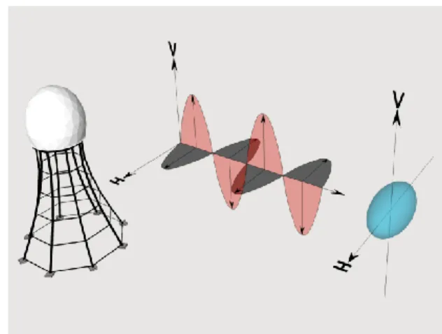
In order to define the phenomenon of polarisation, in case an electromagnetic wave is taken in to account, if the rotation rate of the vector points to frequency and the vector length pointing to the amplitude, then the polarisation is given by the shape and orientation, i.e. whether being horizontal or vertical or of both. Polarimetric radar possesses the ability to transmit and receive both horizontal and vertical orientations of waves. While dual-polarised radars can transmit and receive pulses of orientation HH and VV or HV and VH , completely polarimetric radars can possibly transmit and receive four different combinations of oriented pulses such as HH, VV, HV, VH. The transmission and reception of the waves is less flawed with the latter, for a comparison within the polarimetric radars. Polarisation is classified in to two types such as linear and circular polarisations. Horizontal and vertical orientations can be categorised under linear polarisation. The transmitted horizontal and vertical signals are received by the receiving antennas of their orientation, depending upon their state of polarisation. In case of circular polarisation, the electric forces rotate at 360˚. They usually occur at two phase shifts of 90˚. Due to this they possess two different sides of right and left probably RR and LL respectively.

TARGET APPROACH BY POLARIMETRY

The characteristic change in the transmitted and the received wave accounts to polarisation. The interaction of the transmitted signal with the target focussed decides whether the wave is polarised or depolarised. Depolarisation can be defined as degree of polarisation of a partially polarised wave upon scattering. Whenever the transmitted interacts with the target, part of the signal returns back to the source. The reflected, received signal is termed to be backscattered signal.

Fig 1: waves of horizontal and vertical orientations.

The phenomenon of scattering occurs on hitting the target before reflection. The scattering of the transmitted signal are of three types. If the waves possess simple interaction with the targets, i.e. directly hits the target and returns back, such interaction is termed to be single scattering or the odd bounce scatter. If the scattering occurs between two parts of the target, i.e. the surface level and as well as the stem trunk of a tree then it is termed as double scatter or even bounce. If the scattering level of the wave is more, i.e. scattering through leave and stems apart from ground and trunk level, then it is termed to be multiple scattering. The various levels of scattering are explained in detail with the following fig1. The 1st image is an example of the ingle scattering where B and C refer to the double scattering. The C is an example of multiple scattering where the wave is scattered at ground level, stem and leaves.

(3)

ANALYSATION TECHNIQUES

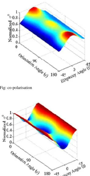
Various analysing techniques are currently under implementation. The estimates are commonly obtained through Synthetic Aperture Radars, Polarimetric radars and Interferometers. While considering SAR measurements, airborne and space borne techniques are generally utilised. Since the synthetic aperture radar have the capability of measuring both amplitude and phase, the differential phase shift is measured by measuring the incident and the reflected wave forms. The length of the pulse determines the resolution of the target range. Hence, the resolution increases with decrease in pulse range. For the purpose of retrieving higher resolution images, the higher level images are intended to impose upon the lower level ones, such that the ambiguity is reduced further (Avril Behan, Iain Woodhouse-1999). While using the principle of Polarimetry, to determine the backscattering, the co polarisation phase difference accounts. The estimate is considered for two different instances, one for single bounce and another to double bounce. While considering the instance of single bounce, the co polarisation phase difference tends to 0˚. For the double bounce, the phase difference tends to 180˚. For a large synthesis condition with a different variety of polarisations, it is not possible to analyse an estimated data. At this state, a three dimensional plot called polarimetric signatures are utilised to graphically determine the backscatter response. They represent linear horizontal polarisation along x-axis and linear vertical polarisation along y-axis. The strength of the backscatter can be computed for the same polarization on transmission and reception. The following figure represents the co-polarization and cross polarization. The x, y and z axis represents the normalized angle, ellipticity angle and orientation angle respectively.

Fig: co-polarisation

Fig 4: cross-polarisation

(4)

Fig 5: a graphical image exhibiting pedestal height.

ALGORITHMS UTILISED FOR CALCULATION:

The biomass estimation above the ground level is given by the relation,

Bg =1_𝐴 𝛱𝐷𝑖2

4 𝐻𝑖𝑊𝑖

𝑖 (1)

And the volume factor is given by,

V =1_𝐴 𝛱𝐷𝑖2

4 𝐻𝑖

𝑖 (2)

Where,

H is the height of the tree,

W is the wood density,

A is the sampled area,

D is the diameter of the height of the trunk part.

Other than the estimation of biomass, the radar backscatter accounts in estimation. Hence, the backscatter is given by,

σ (H,V)= σhead+ σtrunk+ σsurface

(3)

Extending the above equation in terms of the total volume, the forest density, the above equation can be stated as,

σ(

H

,

V

) =

f

(

vol

,

Wd,ω

)

(4)

Where,

Vol= total size of the forest area to be estimated,

Wd= the density of the tree, ω= shape and orientation.

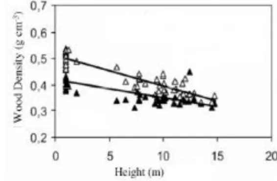
A sample graph is provided below, which is plotted between tree density and height.

Fig: 6 Heights vs. Wood Density

EXAMPLE CASE:

A previously analysed case is taken here as an example for demonstration. The following experiments were conducted and studied by, Sun and Ranson in 2000, Castel in 2001, and Saachi and moghadhaam in 2000. The compared three different values were taken from AIRSAR channels. The polarisations that are provided are HH, VV and HV respectively. The experiments were conducted on tropical rainforests. The bands that were used were of L band and P bands. These two were preferred due to their wavelength of 27 cm for L band and 70 cm for P- band. The comparison is shown between L band and C band is also verified here. The sample of imaging of L and P bands are produced in the following figure,

(5)

Fig 8: An imaging through P-band

And the respective radar back scatter and the biomass estimation with comparison to the l band and the p band are given as follows,

Fig 9: backscatter vs. biomass

For the L band, for complete horizontal orientation, the R² is of 0.27 and for complete vertical orientation, the R² is 0.44, and for both horizontal and vertical aspects the R² is 0.47.

Fig 10: backscatter vs. biomass

For the P band, for complete horizontal orientation, the R² is of 0.79 and for complete vertical orientation, the R² is 0.76, and for both horizontal and vertical aspects the R² is 0.86. On comparing the backscattered values of L and P band with aspect to biomass on various polarisations, it is clearly visible that the correlation is better in both bands. However, the P band is more linear and less attenuated.

CONCLUSION:

Ever since the Polarimetry concept was revealed to the field of forestry, significant approaches of advancement ever made since. They are generally utilised to measure the density of the vegetation and estimation of species. Rather than that, the forests serve something more beneficial. They serve as the home to various rare and extinct animals and invertebrates. They also constitute rare mineral resources over the surface layer, i.e. crust and beneath. They weren’t created over a single day, their presence being estimated for nearly hundreds of years, Even though of rigorous improvements there are still places and priceless constituents that are yet to be harnessed. At this state, the Polarimetry would prove a better solution. Advancement such as immense resistivity towards blockages and improvement in the frequency range would produce polarisation pulses of different orientations at high ranges so that the correlation and stability is maintained high. Many losses shall be avoided.

REFERENCES:

1. Cloude, S. R. & Pottier, E., (1997). An Entropy Based Classification Scheme for Land Applications of Polarimetric SAR.IEEE Transactions on Geoscience and Remote Sensing, Vol. 35, No. 1, pp 68-78.

2. Cloude, S. R. & Pottier, E., (1996). A review of Target Decomposition Theorems in Radar Polarimetry. IEEE Transactions on Geoscience and Remote Sensing, Vol. 34, No. 2, pp 498-517.

3. Cloude, S. R., (1992). Uniqueness of target Decomposition Theorems in Radar Polarimetry. Direct and Inverse Methods in Radar Polarimetry, Part 1, W.-M. Boener et al. (eds.), pp 267-296.

4. Van der Sanden, J. J. (1997) Radar remote sensing to support tropical forest management

(6)

7. Mr. Bharathan Iyer, Mr. P. Venkatesan (2012). Agricultural objectives by polarimetric estimation. 8. Mr. Bharathan Iyer, Mr. P. Venkatesan(2012) polarimetric

radar rainfall estimation.

9. S. R. Cloude and E. Pottier, “An entropy based classification scheme for land applications of polarimetric SAR,” IEEE Trans. Geosci. Remote Sens., vol. 35, no. 1, pp. 68–78, Jan. 1997.

10. S. R. Cloude, J. Fortuny, J. M. Lopez-Sanchez, and A. J. Sieber, “Wideband polarimetric radar inversion studies for vegetation layers,” IEEE Trans. Geosci. Remote Sens., vol. 37, no. 5, pp. 2430–2441, Sep. 1999.

11. D. L. Schuler, J. S. Lee, D. Kasilingam, and G. Nesti, “Surface roughness and slope measurements using polarimetric SAR data,” IEEE Trans. Geosci. Remote Sens., vol. 40, no. 3, pp. 687–698, Mar. 2002.

12. J. S. Lee, D. L. Schuler, T. L. Ainsowrth, E. Krogager, D. Kasilingam, and W. M. Boerner, “On the estimation of radar polarization orientation shifts induced by terrain slopes,” IEEE Trans. Geosci. Remote Sens., vol. 40, no. 1, pp. 30–41, Jan. 2002.

13. . J. van Zyl, “Unsupervised classification of scattering behavior using radar

polarimetry data,” IEEE Trans. Geosci. Remote Sens., vol. 27, no. 1,

pp. 36–45, Jan. 1989.

14. S. R. Cloude and E. Pottier, “A review of target decomposition theorems in radar polarimetry,” IEEE Trans. Geosci. Remote Sens., vol. 34, no. 2 pp. 498– 518, Mar. 1996.

15. A. Freeman and S. L. Durden, “A three-component model for polarimetric

SAR imagery,” IEEE Trans. Geosci. Remote Sens., vol. 34, no. 3,pp. 963–973, May 1998.

16. A. Freeman, “Fitting a two-component scattering model to polarimetric SAR data from forests,” IEEE Trans. Geosci. Remote Sens., vol. 45, no. 8, pp. 2583–2592, Aug. 2007.

17. Y. Yamaguchi, T. Moriyama, M. Ishido, and H. Yamada, “Four component scattering model for polarimetric SAR image decomposition,” IEEE Trans. Geosci. Remote Sens., vol. 43, no. 8, pp. 1699–1706, Aug. 2005. 18. Y. Yamaguchi, Y. Yajima, and H. Yamada, “A

four-component decomposition of POLSAR images based on the coherency matrix,” IEEE Geosci. Remote Sens. Lett., vol. 3, no. 3, pp. 292–296, Jul. 2006.

19. E. Rodriguez and J. M. Martin, “Theory and design of interferometric synthetic aperture radars,” Proc. Inst. Elect. Eng., vol. 139, no. 2 pp. 147–159, Apr. 1992. 20. J. O. Hagberg, L. M. H. Ulander, and J. Askne,

“Repeat-pass SAR interferometry over forested terrain,” IEEE Trans. Geosci. Remote Sens vol. 33, no. 2, pp. 331– 340, Mar. 1995.

21. R. N. Treuhaft, S. N. Madsen, M. Moghaddam, and J. J. van Zyl, “Vegetation characteristics and underlying topography from interferometric

22. radar,” Radio Sci., vol. 31, no. 6, pp. 1449–1485, Nov. 1996

.