Reducing the costs of meeting regional water supply reliability goals through risk-based water transfer agreements

Reducing the costs of meeting regional water supply reliability

goals through risk-based water transfer agreements

By

Reed Palmer

A thesis submitted to the faculty of the University of North Carolina at Chapel

Hill in partial fulfillment of the requirements for the degree of Master of

Science in the Department of Environmental Sciences and Engineering

Chapel Hill

2006

Approved by

Advisor: Dr Gregory W. Characklis

Reader: Dr David H. Moreau

ABSTRACT

REED PALMER: Reducing the costs of meeting regional water supply reliability goals through risk-based water transfer agreements.

(Under the direction of Gregory Characklis)

ACKNOWLEDGEMENTS

I would like to begin by expressing my gratitude to the citizens of North Carolina, past

and present, for placing priority on the development of public institutions of higher

education. Their commitment to these establishments has helped to elevate the University

and this department to the positions of prominence that they hold today. I am grateful to the

University of North Carolina, the Department of Environmental Sciences and Engineering,

and my advisor, Dr. Gregory Characklis for making my graduate education here possible. In

addition, I am thankful for the time and energy Dr. Characklis devoted to me in an effort to

CONTENTS

Page

LIST OF TABLES ……… vi

LIST OF FIGURES ………. vii

LIST OF ABBREVIATIONS AND SYMBOLS ……… viii

Chapter I INTRODUCTION ……… 1

II METHODS ……… 6

2.1 Take-or-Pay Agreements ……… 7

2.2 Days of Supply Remaining Agreements ……… 9

2.3 Risk-of-Failure Agreements ………..… 11

2.4 Reservoir Model ……… 16

2.5 Reliability and Cost ……… 18

2.6 Application of the model to the study region ……… 19

III RESULTS ………...…. 31

3.1 Take-or-Pay Agreements ………...…. 32

3.2 Days of Supply Remaining Agreements ………. 35

3.4 Comparison of Minimum Cost Scenarios ……….. 44

IV FINAL REMARKS ………. 48

APPENDICIES Page A. Comparison of Durham Reservoir Model and Use of Hydro-ram Pumps 49 B. Demand Estimation ………... 54

C. Additional Results……….. 57

D. Risk-of-Failure Tables by week for Durham and OWASA ………….. 64

E. Simulation Codes Used (MATLAB v. 7.0.4) ………. 76

F. Program Code Used to Generate Risk Charts ……….………….. 89

G. Simulation Data ………... ………. 92

LIST OF TABLES

Table Page

1. Sample Risk-of-Failure Chart ………... 13

2. Parameters for OWASA, Durham, Cary/Apex supply systems ………….. 22

3. Size increments and cost for expanding Cary/Apex WTP ………... 26

4. Size, Capacity, and Unit Cost of Pipelines ……….. 26

5. Parameters for Cost Calculations ………. 30

6. Cost Comparison of Take-or-Pay agreements ………. 33

7. Minimum cost solutions for DSR Agreements ……… 36

8. Minimum cost solutions with Risk-of-Failure Agreements ……… 41

9. Comparison of the minimum cost infrastructure/agreement scenarios …… 44

10.Parameters for Estimating Future Demand ……….. 54

LIST OF FIGURES

Figure Page

1. Interconnected utilities and common treatment plant ………..…… 7

2. Sample Risk-of-Failure ………..…. 14

3. Illustration of Weighting Factor ………..… 15

4. Research Triangle Region ………..…. 21

5. Model Storage Curve versus Observed Storage Curve - OWASA ………..…. 23

6. Model Storage Curve versus Observed Storage Curve - Durham ….……..…. 23

7. OWASA Reliability vs. WTP Capacity vs. Cary-Durham Pipeline Capacity … 27 8a. Durham Reliability vs. α threshold values ………... 28

8b. OWASA Reliability vs. α threshold values ………... 29

9. Average Annual Cost of Transfer Programs ……….…….. 30

10a Storage values for α thresholds by week – OWASA ……… 40

10b Storage values for α thresholds by week – Durham ……… 40

LIST OF ABBREVIATIONS AND SYMBOLS

Abbreviations

cfs : Cubic feet per second

DSR : Days of supply remaining (in terms of annual average daily demand) Kgal : Kilogallon or thousand gallons.

MGD : Millions of gallons per day MG/yr : Millions of gallons per year ROF : Risk-of-Failure

WTP : Water treatment plant

Symbols

α : The maximum Risk-of-Failure that a utility is willing to accept before it will request a transfer to offset withdrawals from its own reservoirs

t

i

A : Treatment capacity allocated to utility i in period t.

y

i

b : Average annual demand for utility i in reference year y (base demand). C : Reservoir capacity.

j

i

CC : Conveyance capacity in network segment j allocated for utility i;

j

CC : Total conveyance capacity of network segment j;

Annual

Cap

Cost : Amortized cost of capital investments.

Total

Cap

Cost : Total cost of capital investments in treatment and conveyance infrastructure.

i

d : Annual average daily demand for utility i (MGD);

t

t

i

d : Demand in the ith utility’s service area during period t.

'

t i

d : Demand for utility i in historical period t’.

y i

d : ith utility’s annual average demand for reference year y.

limit

i

DSR : Transfer threshold storage level denoted in Days of Supply Remaining.

i

g : Growth in demand of treated water in utility i (MGD/year); i : Discount rate applied to the principal.

It : Reservoir inflow in period t.

λ : Treatment process loss fraction of raw water withdrawals. Lt : Net evaporation/precipitation from the reservoir during period t.

t

i

N : Contract amount for purchasing utility i in period t. s

NumberYear : Number of years over which the simulation is run

Ot : Reservoir outflow not captured by utility (e.g. minimum release, overflow

spillage, etc.).

i

p : Unit price paid by utility i for water transfers ($/Kgal).

1

−

t

i

S : Storage in ith utility’s reservoirs at the end of time period t-1.

α i

S : Reservoir level corresponding to threshold value α in period t-1.

failure

i

S : Storage level corresponding to the defined failure point.

t

T : Total treatment capacity available for water transfers in period t.

t i

w : Weighting factor applied to utility i determine treatment and conveyance capacity allocation when multiple utilities request transfers in the same period.

t

i

X : Transfer volume to utility i in period t.

y : Number of years over which the capital investments are amortized. y : Base or reference year for projecting future demand.

Y : Target year (for future demand projection).

Chapter I Introduction

As world population continues to grow and economic activity increases, water scarcity is becoming an increasingly important concern. It is estimated that as of 1995 humans appropriated 23% of the readily available fresh water and that by 2025 as much as 70% may be used to serve human demands (Postel, 1996). The high costs and limited opportunities for expanding water supplies have begun to restrain the traditional supply-side approach to water resources planning, while political, social, and economic forces contribute to make it increasingly difficult to develop new water supply sources (Glieck, 1998). All of these influences combine to place growing pressure on water resource managers to use currently available water resources with greater efficiency. The management of uncertain and scarce supplies can be challenging, but efficiency can be improved through the development of increasingly sophisticated approaches (National Research Council, 2001).

be transferred through natural systems (e.g. rivers), man-made structures (e.g. pipelines and aqueducts) or a combination of the two. In addition, water transfers may occur within the context of an established water market (Michelson and Young, 1993; Hamilton et al., 1989), such as those common in the western U.S. (Characklis et al., 1999), or through regional agreements between water utilities (Lund, 1988; Palmer et al, 2001). Indeed, as municipal and industrial water demands have grown, the use of water transfers has expanded as water purveyors work to guarantee supply reliability at lower cost and with fewer environmental impacts than might be the case with strategies involving new water supply projects.

Inter-utility transfers have been employed in the United States for many decades (Lund, 1988; NRC, 1992; Carey and Leonard, 1968), as transfers offer a potentially useful tool for utility managers seeking to reduce the supply capacity they must maintain in order to meet reliability goals. Lund and Isreal (1995) describe the importance of water transfer agreements specifying the location, timing, quantity, and price of the transfer. This requires the development of decision rules that stipulate the conditions under which a transfer is made.

length of time predicted demands can be met with available storage. The probability that an adverse event will occur (e.g. reservoir level declining to an unacceptable level) is another metric that has been incorporated into decision rules (Hirsch, 1978; Moreau, 1991). These studies describe the application of risk-based criteria to the formulation of reservoir operating policies for drought events. Moreau (1991) uses a simulation routine to tune decision rules for progressively staged conservation actions based on the probability that the supply system could satisfy a prescribed set of constraints (e.g. the probability of implementing use restrictions does not exceed a specified threshold).

The decision rules associated with water transfers may be similar in some ways to those designed for reservoir operations, but there will also be important differences. In the case of transferring treated water, it is critical to recognize that the treatment and conveyance infrastructure available to support these transfers will impact the nature of the decision rules necessary to ensure water supply reliability. For example, if infrastructure capacity were not limiting, then a utility might wait until a shortfall was imminent before requesting a transfer as it would be able to quickly acquire vast amounts of water. Conversely, a very limited infrastructure capacity would require a utility to request smaller transfers much more frequently and often well in advance of potential shortages, some of which might not occur. The tradeoffs between infrastructure capacity and the terms of transfer agreements can be fine-tuned through refinement of the decision rules in these agreements and lead to infrastructure-agreement combinations that can lower the costs of meeting supply reliability objectives.

factor (Dinar et al., 1997; Wilchfort and Lund 1997; Characklis and Kirsch et al., 2006). This research explores tradeoffs between the structure of transfer agreements and the infrastructure needed to support the transfers, with the decision rules governing the transfer agreements playing a critical role. These tradeoffs are explored for several different types of agreements, with the minimum cost combination of agreement and infrastructure identified in each case.

The subjects of this study are three urban water agencies in the Research Triangle region of North Carolina. This is an area of rapid urbanization with commensurate growth in water demand (US Census Bureau, 2005; NC DWR, 2001). The region has traditionally relied on surface water reservoirs for its supply, yet the expansion of reservoir capacity in North Carolina has slowed dramatically in recent years (Moreau, 1992). The combination of rapid growth and limited options for new supply development make it a fitting region to evaluate the role that inter-utility water transfers can play in the development of water resource management strategies.

agreement uses a decision rule that incorporates use of historical hydrologic records to estimate the “Risk of Failure” (where failure is defined as a particular storage level) for a given utility such that a transfer can be requested whenever this risk exceeds a specified threshold.

Chapter II Methods

2.1. Take-or-Pay Agreements

A “Take-or-Pay” agreement specifies a fixed amount of water that will be available to the buyer over a certain period of time, without consideration of hydrologic conditions. Some variation of this type of agreement is currently used by many utilities. With Take-or-Pay agreements the seller typically commits to provide the buyer with a specified amount of water at all times and the buyer commits to paying for this amount, whether or not the buyer actually requests a transfer. In this case the buyer’s decision is simple, and it will request the maximum volume specified in the contract any time its own reservoirs are less than full. When the buyer requests a transfer, there are three principal factors that determine the transfer volume: 1. the maximum volume specified in the contract; 2. the available treatment capacity; 3. the conveyance capacity available. If the available treatment capacity or conveyance capacity are not sufficient, it may not be possible to deliver the maximum amount specified in the contract. In situations where more than one utility may be purchasing transferred water, the method of apportioning the available treatment capacity and conveyance capacity is also important. In this case, both treatment and conveyance capacity are allocated in proportion to the maximum quantities specified in each contract. For example, suppose that a number of utilities are aligned in a series along a common pipeline connected to a water treatment plant as shown in Figure 1.

i=1

Treatment plant

i=1

Figure 1: Interconnected utilities and common treatment plant

j=m i=2

The capacity allocation process begins with the most distant utility, n, such that:

∑

=

= _n

i i

i t i

t t t

N N T A

1

[1]

where,

i : index of purchasing utilities, i = 1, 2, 3, ….n;

t

i

A : treatment capacity allocation for purchasing utility i in period t ;

t

T : total treatment capacity available for water transfers in period t;

t

i

N : contract amount for purchasing utility i in period t;

Similarly, the segments of the conveyance network are shared by multiple utilities with the capacity allocated to utility i in network segment j expressed as:

∑

=

= _n

i i i j i

t t j

N N CC CC

1

[2]

where,

j : index of conveyance network segments j = 1, 2, 3, … m.

j

i

CC : conveyance capacity in network segment j allocated for utility i;

j

CC : total conveyance capacity of network segment j;

t

i

This calculation is repeated for each network segment through which a transfer from the treatment plant to utility i must pass. The maximum transfer size available to the purchasing utility, i, is the smallest of these values CC_ijsuch that:

CC_i =min[CC_ij] over all segments j = 1, 2, 3, … m. [3]

The maximum transfer to utility i in period t ( ) then becomes the smallest volume allowable within these three constraints (i.e. treatment, conveyance, contract) such that

t

i

X

min =

t

i

X [A_it,CC_i,N_it] [4]

This process, which begins with [1] and the most distant utility is repeated for the next most distant utility, adjusting the available treatment and conveyance capacities to account for that already assigned to the more distant utilities.

2.2. Days of Supply Remaining

The second type of agreement examined uses a decision rule based on the Days of Supply Remaining (DSR) in the purchasing utility’s reservoir(s) to determine when transfers will be requested. A similar hedging rule has been developed to manage reservoirs under drought contingencies (Fisher and Palmer 1997). A water transfer is requested in any period in which reservoir storage at the end of the previous period, is less than a pre-determined level such that,

1

−

t

i

if , then the utility will request a transfer [5] t imi l t i i DSR

DSR₋ <

1 where, i i i d S DSR t t 1 1 −

− = [6]

1

−

t

i

S : the storage in ith utility’s reservoirs at the end of time period t-1;

i

d : annual average daily demand for utility i;

limit

i

DSR : the transfer “trigger” storage level.

When the DSR decision rule triggers a transfer request, the amount requested is for an amount up to the utility’s demand in period t, . If only one utility requests a transfer during the period, the quantity actually transferred is determined by the lesser of the constraints on treatment and conveyance capacities, up to the entire demand for utility i in period t, such that,

t

i

d

[ ] [7]

min = t i X t i i

t CC d

T, , where,

: demand in the ith utility’s service area during period t.

t

i

d

During periods in which multiple utilities request a transfer, the allocation method used with the DSR decision rule assigns the available treatment capacity, , in proportion to the average demand of each utility such that,

t

T

∑

=

= _n

i i i t i

d d T A_t

1

[8]

Similarly, conveyance capacity is allocated over each segment j such that,

∑

=

= _n

i i i j i

d d CC CC

j

1

[9]

As with the Take-or-Pay agreement, this calculation is repeated for each network segment through which a transfer from the treatment plant to utility i must pass. The maximum conveyance capacity available to the purchasing utility, i, is the least of all the values as described in [3]. The maximum transfer volume to utility i, in period t is then given by minimum:

j

i

CC

min =

t

i

X [A_it,CC_i ,d_it] [10]

2.3. Risk-of-Failure

Table 1: Sample Risk-of-Failure Chart for the following 12 months for a given storage level and month of year

Beginning Reservoir

Level Jan Feb Mar Apr May Jun Jul Aug Sep Oct Nov Dec

100% 0% 3% 3% 3% 3% 1% 0% 0% 0% 0% 0% 0%

95% 0% 3% 3% 3% 3% 3% 1% 0% 0% 0% 0% 0%

90% 0% 3% 3% 3% 3% 3% 1% 0% 0% 0% 0% 0%

85% 0% 3% 3% 3% 4% 3% 3% 0% 1% 1% 0% 0%

80% 0% 3% 3% 5% 5% 3% 4% 4% 1% 1% 0% 0%

75% 0% 3% 4% 6% 6% 6% 8% 5% 3% 1% 1% 0%

70% 0% 4% 5% 6% 13% 13% 9% 6% 4% 1% 1% 0%

65% 0% 4% 5% 9% 14% 17% 16% 10% 4% 1% 1% 0%

60% 0% 4% 5% 9% 19% 23% 19% 14% 5% 3% 1% 1%

55% 1% 5% 6% 13% 25% 30% 27% 22% 10% 4% 1% 1%

50% 1% 6% 8% 16% 29% 36% 32% 29% 21% 5% 1% 1%

45% 1% 6% 9% 18% 39% 45% 42% 38% 29% 9% 4% 1%

40% 1% 8% 12% 22% 40% 47% 45% 45% 43% 23% 4% 1%

35% 4% 9% 13% 27% 47% 48% 49% 49% 52% 34% 9% 4%

30% 6% 9% 13% 34% 49% 55% 56% 57% 62% 51% 18% 5%

25% 10% 9% 17% 35% 52% 69% 66% 70% 70% 65% 42% 14%

20% 16% 10% 18% 39% 57% 74% 77% 77% 78% 70% 55% 22%

15% 21% 17% 19% 44% 62% 77% 79% 77% 82% 73% 65% 29%

10% 27% 25% 22% 48% 69% 83% 88% 83% 86% 81% 68% 43%

5% 32% 27% 25% 52% 78% 88% 90% 88% 86% 86% 70% 52%

0% 39% 29% 31% 56% 83% 94% 91% 91% 88% 87% 75% 61%

Jan Feb Mar Apr May June July Aug Sept Oct Nov Dec 0.0%

10.0% 20.0% 30.0% 40.0% 50.0% 60.0% 70.0% 80.0% 90.0% 100.0%

R

e

srvoir Stora

ge Level

1% Risk-of-Failure

5% Risk-of-Failure

10% Risk-of-Failure

Figure 2: Sample Risk-of-Failure for a system with high inflows and low demand during winter months.

Using Risk-of-Failure as a decision rule involves the utility setting a maximum risk tolerance threshold, α, such that,

if Risk-of-Failure > α , then the utility will request a transfer

the allocation in favor of a utility that is relatively worse off than others in the system. The weighting factor is expressed as:

failure t

t t

i i

i i i

S S

S S w

− − =

− −

1 1

α _[11]

where

: reservoir level corresponding to threshold value

α i

S α in period t-1;

: storage level at the end of period t-1;

1

−

t

i

S

: storage level correspondings to the defined failure point.

failure

i

S

Each utility’s weighting factor will increase rapidly as reservoir levels approach the defined failure point, S_ifailure , as illustrated in Figure 3, below.

This weighting factor is applied to the allocation for treatment plant capacity, such that:

∑

∑

The same weighting factor is also used to allocate pipeline capacity, such that:

∑

∑

The transfer volume for the utility i in period t is then determined using [10].

2.4 Reservoir Modeling

A traditional reservoir model serves as the basis for the simulation and takes the form:

t t t t 1 -t

t S I - W -O -L

S = + [14]

where

St : reservoir storage at the end of time period t, 0 ≤ St ≤ C;

It : reservoir inflow in period t;

Wt : withdrawals in period t;

Ot : reservoir outflow not captured by utility (e.g. minimum release, overflow

spillage, etc.);

Lt : net evaporation/precipitation loss/gain from the reservoir during period t;

Reservoir withdrawals (Wt) typically exceed treated water production by a small margin

due to process losses during treatment, such that:

( )

d

W t

t = [15]

where

: demand for treated water in period t;

t

d

λ : loss fraction.

When inter-utility transfers ( ) are incorporated into the model the withdrawals made by a utility are reduced by the amount of treated water received in the transfer such that,

t

i

X

(

)

X d

W t t

t

−

= [16]

The reservoir model described in [14] is modified to incorporate consideration of transfers such that:

t t t t t 1 -t

t -O -L

-1

X -d -I S

S ⎟

⎠ ⎞ ⎜

⎝ ⎛ + =

2.5 Reliability and Cost

Each utility’s reliability is defined as,

Reliability = 1 - ⎟

⎠ ⎞ ⎜

⎝ ⎛

Periods of

Number

Failures of

Number

[18]

Failure of the supply system can be defined in a variety of ways (McIntyre, Lees et al. 2003), but for the purposes of this simulation, a failure is recorded anytime a utility’s cumulative storage is less than 20% of working capacity. Conversely, to characterize the supply system as reliable for a particular period, demand must be met in full and the cumulative storage must be equal to or greater than 20% of working capacity. Using a storage level of 20% as the threshold for failure (rather than 0% capacity) provides the utilities with some margin of safety and seems to be a heuristic rule used to guide the utilities assessed in this work. Other definitions of failure could easily be considered in this framework.

The cost of the transfer program includes the amortized capital cost of the water treatment and conveyance infrastructure, as well as the agreed upon purchase price for treated water. When comparing the costs of the three types of agreement, an annual average cost is calculated. With respect to the agreements using DSR or Risk-of-Failure decision rules, maximum, and average annual cost are also calculated. Annualized capital costs (Cost_CapAnnual) are calculated using a capital recovery factor such that

( )

⎠ ⎞ ⎜⎜

⎝ ⎛

+ −

= _{Cap −y}

Cap

i i Cost

Cost

Total Annual

1

1 [19]

where

Total

Cap

y : number of years over which the capital investments are amortized.

The average annual cost of water transfers is computed as,

s NumberYear

p X Cost

z

t n

i i i

Transfer

t

Annual

∑∑

= =

= 0 1 _[20]

where,

: number of discrete periods in the simulation; z

: unit price paid by utility i for water transfers;

i

p

: number of years over which the simulation is run.

s NumberYear

The average annual cost of the transfer program is the sum of [19] and [20].

2.6. Application of the model to the study region

Table 2: Parameters for OWASA, Durham, Cary/Apex supply systems

System Parameter Assumed Value

OWASA Working volume of Cane Creek Reservoir 2910 MG

Working volume of University Lake 449 MG

Working volume of Stone Quarry 198 MG

Total working volume 3357 MG

Working volume at failure point 711 MG

Cane Creek Reservoir Minimum Release (inflow < 0.22 cfs) 0.22 cfs or 0.14 MGD Cane Creek Reservoir Minimum Release (inflow > 2.78 cfs) 2.78 cfs or 1.8 MGD Cane Creek Reservoir Minimum Release 0.22 cfs < inflow < 2.78 cfs Equal to inflow University Lake and Stone Quarry Minimum Release None or 0 MGD

Durham Working volume of Lake Michie 3300 MG

Working volume of Little River Reservoir 4900 MG

Total working volume 8200 MG

Working volume at failure point 1851 MG

Little River Reservoir Minimum Release (June – Nov) 2 cfs or 1.3 MGD Little River Reservoir Minimum Release (Dec – May) 6 cfs or 3.8 MGD Little River Reservoir Minimum Reservoir (anytime storage < 70%) 0.64 cfs or 0.4 MGD

Lake Michie Minimum Release None or 0 MGD

Cary/Apex Water Treatment Plant Process Loss 13%

Treatment Plant Capacity (as of 2006) 40 MGD

scenarios discussed in Chapter III, transfers were added to the demand in the purchasing utility’s service area.

0.0% 10.0% 20.0% 30.0% 40.0% 50.0% 60.0% 70.0% 80.0% 90.0% 100.0%

1/1/1996 1/1/1997 1/1/1998 1/1/1999 1/1/2000 1/1/2001 1/1/2002 1/1/2003 1/1/2004 1/1/2005 Model Storage Curve

Actual Storage

Figure 5: Model Storage Curve versus Observed Storage in OWASA’s Reservoir System

0% 20% 40% 60% 80% 100% 120%

1/1/2000 1/1/2001 1/1/2002 1/1/2003 1/1/2004 1/1/2005 Model Storage Curve

Actual Storage

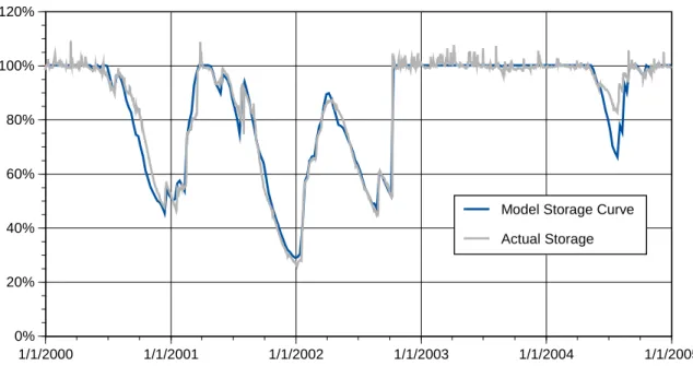
Figure 5 represents aggregate storage in OWASA’s three reservoirs (University Lake, Cane Creek Reservoir, and Stone Quarry) as a percentage of the total storage capacity, but it should be noted that the model treats inflows and withdrawals from the three reservoirs separately. The standard error between OWASA’s modeled and observed storage levels over the 15 year period is 0.044. Durham’s supply system consists of two reservoirs, Lake Michie and Little River Reservoir, with Figure 6 representing the aggregate storage in both reservoirs. Results suggest good agreement between model and observed storage levels, but arriving at the appropriate comparison was complicated by their intermittent use of hydraulic ram pumps to deliver raw water to the treatment plants. Hydraulic-ram pumps have a large bypass (i.e. undelivered fraction) which had to be calibrated (for further explanation of this situation see Appendix B). After accounting for effects of these pumps, the standard error between modeled and observed storage was 0.037, a value deemed suitable for this work.

The safe yield of the water supply pool of Jordan Lake is estimated to be at least 100 MGD, and OWASA and Durham have allotments of 5% and 10% of the water supply pool, respectively. Therefore, for the purposes of this study the supply on Jordan Lake is assumed to be sufficient to accommodate transfers averaging up to 5 MGD and 10 MGD to OWASA and Durham, respectively.

The simulation is used to test each of the different types of transfer agreement over a range of different infrastructure capacities (both treatment plant and conveyance), and to evaluate the total cost and supply reliability associated with each agreement/infrastructure combination. The primary factors affecting the supply reliability and transfer program cost of each scenario modeled are:

(2) Cary to Durham pipeline capacity (3) Durham to OWASA pipeline capacity (4) Demand (i.e. which target year is simulated) (5) Agreement Type/Terms

(a) The size and timing of the contract (for Take-or-Pay contracts) (b) The threshold values selected (DSR and Risk-of-Failure)

week of the year (late May) and continue through the 50th week (mid-December). Those set to coincide with the refill period run from week 51 through week 21 of the following year. These three strategies were evaluated using 2030 profiles for each of the utilities and increasing transfer volumes incrementally until each utility reached 100% reliability.

The approach taken for determining the most cost-effective DSR and Risk-of-Failure agreements is somewhat more complex because of the tradeoff between increased infrastructure capacity (i.e. capital cost) and the ability to wait longer before requesting transfers, which on average will reduce transfer costs.

When considering infrastructure capacity alternatives there are a limited number of discrete sizes that could practically be selected. The size and cost of those discrete choices are outlined in Tables 3 and 4, below.

Table 3: Size increments and cost for expanding Cary/Apex WTP (Hazen and Sawyer, 2004) Raw water

Capacity

40 MGD 48 MGD 56 MGD 64 MGD 72 MGD 80 MGD

Incremental Cost

$3,201,0001 _$22,218,0002 _{$9,172,000 $39,907,000}3 _{$9,763,000 $9,485,000}

Total Cost $3,201,000 $25,419,000 $34,519,000 $74,498,000 $84,261,000 $93,746,000 1 - Recommended upgrades and improvements

2 - Includes new ozonation facilities to 80 MGD capacity

3 - Includes new intake facilities on Jordan Lake to 80 MGD capacity

Table 4: Size, Capacity, and Unit Cost of Pipelines Pipeline Diameter

(inches)

Conveyance Capacity * _{Installed Cost}

(per linear foot)

12” 2.5 MGD $35

16” 4.5 MGD $50

20” 7.0 MGD $75

24” 10.1 MGD $100

30” 15.9 MGD $120

36” 22.8 MGD $135

42” 31.1 MGD $150

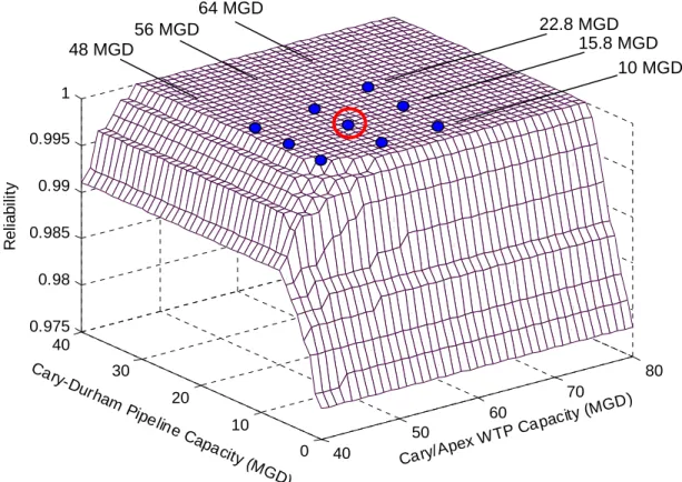
With six different WTP capacities and eight different potential capacities for the two pipelines, there are 384 potential infrastructure combinations. A preliminary investigation revealed that only a limited number were capable of achieving 100% reliability for any agreement type at a competitive cost and these were selected for further investigation. Figure 7 displays an example of the relationship between infrastructure and reliability for OWASA.

Figure 7: Reliability for OWASA. Year 2030 Demand. OWASA Risk-of-Failure threshold 5%. OWASA Risk-of-Failure threshold 13%. Durham to OWASA Pipeline Capacity 7 MGD

The nine points indicated in Figure 7 represent discrete infrastructure combinations that are then each evaluated independently while holding the infrastructure capacity fixed.

40

50

60

70

80

0 10

20 30

40 0.975 0.98 0.985 0.99 0.995 1

Cary/Ape

x WTP C

apacity (M

GD)

Cary

-Dur_ham Pip_elin

e C apa

city (_MG D)

R

e

lia

b

ilit

y

48 MGD

56 MGD

64 MGD

22.8 MGD 15.8 MGD

utilities were able to achieve 100% reliability received further consideration. Figure 8a and 8b show the relationship between reliability and the agreement terms for a Risk-of-Failure agreement for the infrastructure combination circled in Figure 7 (56/15.8/7.0 [Cary/Apex WTP capacity/ Cary to Durham pipeline capacity/ Durham to OWASA pipeline capacity, respectively]). The overlapping region of α thresholds which allow both utilities to reach 100% reliability is noted in Figure 8b. It is this range of agreement terms which receives further consideration.

0 20

40 60

80 0

20

40

60

80 0.996

0.997 0.998 0.999 1 1.001

R

e

lia

b

ilit

y

α

α

0 20

40 60

80 0

20

Region of Mutual 100% Reliability

Figure 8b: Reliability for OWASA vs threshold levels. Year 2030 Demand. 56/15.8/7.0 infrastructure combination.

Figure 9 shows the relationship between average annual program cost and the threshold level, α, selected by each utility. Note that regions where annual average cost is not displayed on Figure 9 indicate combinations of α for which 100% reliability was not attained by at least one of the utilities over the simulation period. So in this particular case, the lowest cost combination ($4.35 million/yr) of α values for which both utilities achieve 100% reliability is α_OWASA of 10% and α_Durham of 32%. This process was repeated over the array of available infrastructure combinations to explore the relationship between infrastructure, agreement, reliability, and average annual cost. This procedure allows the user to determine cost-effective combinations of infrastructure and agreement types that meet reliability

40

60

80 0.975

0.98 0.985 0.99 0.995 1 1.005

R

e

liabi

lit

y

α

0 10

20

Figure 9: Annual Cost of Transfer Programs . Year 2030 Demand. 56/15. .0 infra cture combination.

in able 5, below.

Ta

Parameter Symbol Assumed Value

8/7 stru

Values for the parameters needed to solve for average annual program cost are shown T

ble 5: Parameter values for equations [19] and [20]

Discount rate i 6%

Amortization period y 20 years

Length of Cary-Durham Pipeline - 10 miles Length of Durham-OWASA Pipeline - 5 miles Number of weeks in each simulation z 780 Purchase price paid by OWASA p_i $2.81/Kgal1 Purchase price paid by Durham p_i $2.21/Kgal1

s betw utilities. Pipeline maintenance and 1 – Prices for transferred water based on past transaction een these

30 40

0

5

10

15

20 4

6 8 10 12

x 106

A

v

er

ag

e A

n

n

ual

P

ro

g

ra

m

C

o

s

t

α

rham Minimum cost

Chapter III Results

Results for each of the three agreemen resented primarily in terms of:

1. The infrastructure needed to reac reliability over the 15-year (1990-2004)

3. for each agreement (i.e. contract size and timing for Take-or-Pay .

Nev

program nticipated in the Year 2030, a point at

reliability of 97.8% over the period 1990-2004, t types are p

h 100% simulation period.

2. The average annual cost of the transfer program over the simulation period. The decision rules

agreements, and transfer thresholds for DSR and Risk-of-Failure agreements)

4. If the transfer agreement can be guaranteed, and if not, the percentage of weeks in which the agreement would be interrupted.

ertheless, other metrics are also included to characterize the performance of the transfer s. Results are presented for demand levels a

which both Durham and OWASA may have significant transfer needs depending on hydrologic conditions. A critical assumption implicit within these results is that Durham will discontinue the use of its hydroram pumps on Lake Michie. For an analysis that includes the continued use of these pumps, see Appendix C. Appendix A also covers scenarios pertaining to other demand levels, alternative sales scenarios, and uncertainty regarding the accessible volume of water in Durham’s reservoirs.

42

Each of the three schedules for Take-or-Pay agreements were evaluated: Year Round, Dec 16th), and Refill Phase (Dec 17th – May 27th). Table 6 escribes the details of Take-or-Pay contracts that will allow Durham and OWASA to reach 10

.96 MGD. This represents the “baseline” scenario used to explore the infrastructure and agreement type/terms required for both utilities to achieve 100% weekly reliability over the 15 year hydrologic sequence.

3.1 Take-or-Pay Agreements

Drawdown Phase (May 28th – d

Table 6: Cost Comparison of Take-or-Pay agreements

Ta

Year-Round

ke-or-Pay Drawdown-phase Take-or-Pay

WTP plant capacity 64 MGD 56 MGD 48 MGD 64 MGD 56 MGD 48 MGD

Contract Amount - Durham 1.5 MGD 1.5 MGD 1.5 MGD 1.5 MGD 1.5 MGD 2 MGD Contract Amount - OWASA 3.5 MGD 3.5 MGD 4 MGD 5.5 MGD 5.5 MGD 6 MGD

Annualized Capital Costs (millions) $7.0 $3.5 $2.7 $7.0 $3.5 $2.85

Annual Contract – Durham (millions) $1.2 $1.2 $1.2 $0.7 $0.7 $0.85

Annual Contract - OWASA

(millions) $3.6 $3.6 $4.0 $3.1 $3.1 $3.2

Max OWASA Avg

OWASA T

T / (MG/yr) _{832 / 1201 831 / 1200 908 / 1240 921 / 1066 921 / 1066} 975 / 1218 Freq Max OWASA Freq Avg OWASA T

T . _/ . _{(weeks per year) 34 / 49 34 / 49 33 / 46 25 / 29 25 / 29 24 / 29}

Max Durham Avg

Durham T

T / (MG/yr) 249 / 431 249 / 430 239 / 390 236 / 331 235 / 331 249 / 378

Freq Max Durham Freq Avg Durham T

T . _/ . _{(weeks per year) 24 / 41 24 / 41 23 / 38 19 / 27 19 / 27 19 / 27}

Interruptions 0% 0.25% 4% 0% 1.6% 14%

CapC-D _{(MGD) 7.0 7.0 7.0 7.0 7.0 10.1}

CapD-O _{(MGD) 4.5 4.5 4.5 7.0 7.0 7.0}

Total Annual Cost (millions) $11.8 $8.3 $7.9 $10.8 $7.3 $6.9 Max

i Avg

i T

T / - Average and maximum volume of transfers actually received by the utility on calendar year basis. However, utilities pay for the right to obtain the maximum contract amount but only call it when reservoirs are less than 100% full.

- Average and maximum number of weeks per year the utility engages in transfers. Contract is exercised any time reservoirs are less than 100% full and contract is in effect.

Interruptions – The percentage of weeks in which the full contract amount can not be delivered due to the priority of meeting demand in the Cary/Apex service area. A contract interruption is not indicative of a “failure” or week in which reliability is not met. However, it does indicate the purchasing utility will rely more heavily on its own reservoir system during weeks in which interruptions occur.

CapC-D _{– Minimum size pipeline from Cary to Durham required (See Table 4 for discrete pipeline sizes)}

CapD-O _{– Minimum size pipeline from Durham-OWASA required}

Since the transfer volume is specified in the contract and both buyers can request a transfer at any time the contract is in effect (year-round or during the drawdown phase), the Cary to Durham pipeline capacity required to support the contract is simply the sum of the contract flow rates for OWASA and Durham. The more critical issue is the tradeoff between guaranteeing sufficient treatment plant capacity to meet contract obligations and the increased expense of providing the capacity to do so. Cary/Apex’s annual average demand in 2030 is 28.3 MGD and the highest weekly demand to annual average demand ratio is 1.60,

Freq Max i Freq Avg i T

treatment process loss of 13% based on historical records, this requires 51.3 MGD of raw

w capacity. Thou m a t h

ak day C i e

qu to 54 GD if ted water storage is not used to t peak. To guarantee processing capacity to meet either the year round or drawdown phase agreem

However, both Durham and OWASA can reach 100%

WTP at Cary/Apex if will e w s the fer contract ith a 56 MGD WTP, a -round ent of 1.5 MGD for Durham

and 3.5 M be

fully ughly once in 8 years, due to the priority of fully meeting

dem those weeks,

how

also both utilities to

MGD for Durham). Because this agreement is executed during the summer when demand is highest and the total contract amount is larger than the year-round agreement, interruptions would be higher than for a year-round agreement, occurring in 1.6% of weeks, during which a minimum of 60% of the contract amount would be delivered.

Finally, it is possible for both Durham and OWASA to achieve 100% reliability using either year-round or drawdown-phase agreements and a WTP capacity of only 48 MGD. However, this requires accepting a higher percentage of weeks in which the contract will be interrupted and increasing the contract size by 0.5 MGD to make up for the contract portion

ater processing gh this odel functions on weekly ime step, it is wort keeping in mind that a pe ratio for ary/Apex is even h gher (1.7) and could push th raw water processing capacity re ired .4 M trea

offset tha

ents without interruption requires a 64 MGD WTP capacity. reliability with less expense by relying

on a smaller they accept that in som eek trans

will not be fulfilled. W year agreem

GD for OWASA (the minimum required to reach 100% reliability) would fail to met in 0.25% of weeks, or ro

and in the Cary/Apex service area before making transfers. Even in

ever, 80% of the contract amount could still be delivered. A 56 MGD WTP capacity is needed to support the smallest drawdown phase agreement needed for

that is undelivered in high demand weeks at Cary/Apex. With a WTP capacity of 48 MGD, a drawdown phase agreement would be interrupted in just under 14% of weeks and in roughly a third of those weeks (i.e. 4%) when the agreement cannot be fulfilled, the amount delivered would be less than half of the maximum specified by the agreement. While an interruptible contract may be less desirable than a guaranteed contract, the net effect is to reduce the average annual cost of the transfer program on the order of $400,000 per year from a program using a 56 MGD WTP and by $3.9 million over programs using a 64 MGD WTP. The least costly Take-or-Pay agreement that provides 100% reliability is the drawdown phase agreement with a 48/10.1/7.0 MGD (Cary/Apex WTP capacity/ Cary to Durham pipeline capacity/ Durham to OWASA pipeline capacity, respectively) infrastructure capacity and contract sizes of 6 MGD and 2 MGD for OWASA and Durham, respectively. .

The timing of Take-or-Pay agreements has an impact on the overall cost of the transfer program. Drawdown phase agreements are more cost-effective in general because there is a greater probability they will actually offset demand when reservoir levels are less than full. In a region such as the Research Triangle, where reservoir capacity is limited and/or the refill phase is occasionally insufficient, minimizing the drawdown is the most effective means of improving reliability. In this case, a drawdown phase transfer program saves roughly $1 million per year relative to the year round transfer program.

3.2 Days of Supply Remaining Agreements

Table 7: Minimum cost solutions for DSR Agreements

Cary-Durham Pipeline Capacity Cary/Apex WTP Capacity

7 MGD 10.1 MGD 15.8 MGD 22.8 MGD

48 MGD

OWASA

OWASA

(MG/yr)

C (millions)

88 / 468

$4.08

122 / 614

$4.30

167 / 766

$4.46

168 / 772

$4.54 DSR

DSRDurham

Max

Avg _T

T / (MG/yr)

Freq Max OWASA Freq Avg OWASA T

T . _/ .

Freq Max Durham Freq Avg Durham T

T . _/ .

Interruptions CapD-O (MGD)

Avg

CMax _(millions)

190 79 412 / 1155 11 / 38

2.3 / 14 12% 7.0

$7.01

190 79 419 / 1197 10 / 37

2.3 / 14 15% 7.0

$7.56

186 79 409 / 1193 10 / 36

2.3 / 14 14% 7.0

$7.98

186 79 413 / 1197 10 / 34

2.3 / 14 14% 7.0 $8.07 OWASA Max Durham Avg Durham T T / 56 MGD OWASA OWASA (MG/yr)

C (millions)

84 / 444

$4.72

91 / 508

$4.69

90 / 503

$4.61

116 / 626

5% 10.1 $4.70 DSR DSRDurham Max Avg _T

T / (MG/yr)

Freq Max OWASA Freq Avg OWASA T

T . _/ .

Freq Max Durham Freq Avg Durham T

T . _/ .

Interruptions CapD-O _(MGD)

Avg

178 76 359 / 1185 9 / 36

2.2 / 13 2% 7.0

150 70 281 / 1095 6 / 26

1.6 / 10 4% 10.1

134 61 218 / 1173 4 / 24

1.1 / 7 5% 10.1

130 61 206 / 1181 4 / 23

1.1 / 7

OWASA Max Durham Avg Durham T T /

CMax _{(millions) $7.83 $7.90 $8.20 $8.56}

64 MGD

OWASA

OWASA

(MG/yr)

Interruptions

C (millions)

84 / 444

0%

$8.21

75 / 425

0%

$7.94

93 / 546

0%

$7.97

83 / 568

0% $8.00 DSR DSRDurham Max Avg _T

T / (MG/yr)

Freq Max OWASA Freq Avg OWASA T

T . _/ .

Max Freq Max Durham Freq Avg Durham T

T . _/ .

CapD-O _(MGD)

Avg

CMax _(millions)

178 76 360 / 1210 9 / 36

2.2 / 13

7.0

$11.39

134 64 209 / 1156 4 / 24

1.3/ 8

10.1

$11.37

122 61 176 / 1249 3 / 23

1.1 / 7

10.1

$11.99

114 55 167 / 1361 3 / 23

0.7 / 5

10.1 $12.42 OWASA Durham Avg Durham T T /

DSR – transfer decision threshold

DSRDurham – transfer decision threshold

Max Avg _T

T / - Average and maximum volume of transfers received by the utility on ca

OWASA

lendar year basis

Freq Max i Freq Avg i T .

. _{/ - Average and maximum number of weeks per year the utility engages in transfers.}

terruptions – The percentage of weeks in which an average of 8 MGD of transfers can not be delivered pex service area. Although the amount transferred in any

purposes the agreement is considered to be interrupted in any week in which transfers are requested by either utility and less than 8 MGD for transfers are available (7 MGD for cases in which the Cary to Durham pipeline is only 7 MGD)

Ca

Avg

i i

T

In

due to priority of meeting demand in the Cary/A week is only limited by equation [7], for planning

pD-O _{– The capacity of the Durham-OWASA pipeline that results in the minimum program cost in}

combination with the indicated WTP and Cary to Durham pipeline capacities. C – Average annual cost of the transfer program

The lowest cost scenario includes a 48/10.1/7.0 MGD (Cary/Apex WTP capacity / Cary to

Durham pipeline capacity / Durham to A y)

infrastructure capacity, a er thresho

Under this scenario OWASA receives an averag 19 M of w ansf m Cary/Apex, and a maximum of 1155 M /yr whi stin ers ver 1 weeks/yr and a maximu s/yr. Durham eived age o

maximum of 468 MG/yr, requesting ansfers an av ore

year up to a maximum of 14 weeks/yr a p as

estimated at $4.08 million rising to $7.01 m llion most expensive Thi st cost DSR agreement is an interruptible agreeme ent eptance of interruptions (less than 7 MGD delivered) in about 12% of weeks in which re s are

It is important to note that treatment capacity of a GD at

Cary/Apex is sufficient to meet the transfer n of

simulated weeks (8 of 780 weeks) the dem rvice area alone would exceed the treated water production cap city of t . In f th ht w e demand exceeded treatm y 3 MGD. Therefore, unless Cary/Apex’s peak use

acity is availab P

may not b

DSR thre

exception to this is when using a 7 MGD pipeline between Cary and Durham, the

inc changes in the amount

MGD WTP is of sufficient size to meet OWAS pipeline capacity, respectivel nd transf lds of DSR_OWASAlimit= 190 and DSR_Durhamlimit = 79.

e of 4 G/yr ater tr ers fro G le reque g transf on an a age of 1 m o 38 weekf rec aver f 88 MG/yr and a

tr erage of slightly m than 2 weeks per . The average annu l cost of this transfer rogram w

i in the year. s lowe

nt that ails acc

quest made.

although the excess 48 M WTP

needs of Durham a d OWASA, in 1% and in the Cary/Apex se

a he WTP two o ose eig eeks th

ent capacity b

ratios are reduced or significant treated water storage cap le, a 48 MGD WT e sufficient for meeting their own demand.

As treatment plant capacity increases it allows Durham and OWASA to adopt lower sholds, which in turn reduces the average amount purchased by each utility. The only

Ca

mbination. In addition to the ab

in size from 56

er the frequency with which transfers are

ry/Apex’s demand and produce an additional 7 MGD to transfer to Durham and/or OWASA in almost all situations. This indicates the Cary to Durham pipeline has become the limiting factor with the 64/7.0/7.0 infrastructure co ility to adopt lower DSR thresholds, greater treatment plant capacity affords the purchasing utilities a lower chance that the transfer agreement will be interrupted in any given week. The likelihood that treatment capacity available for transfers is less than 8 MGD (or 7 MGD if the Cary to Durham pipeline has 7 MGD of capacity) drops from 12-15% with a 48 MGD WTP, to 2-5% with a 56 MGD WTP, and to 0% with a 64 MGD WTP. However, treatment plant expansions are expensive and raise the average cost of the transfer program in all cases. This is because the incremental cost in the treatment plant is greater than the amount saved by lowering DSR thresholds and transferring less water. The incremental increase

MGD to 64 MGD is especially expensive because it requires building a larger intake structure on Jordan Lake (See Table 3) and pipeline to deliver raw water to the WTP and produces a $3.5 million increase in the amortized cost of infrastructure.

Building a larger pipeline does not impact the infrastructure cost as drastically as the expansions in the WTP. Even so, the effect of increasing pipeline size on transfer program cost is somewhat complex because of two opposing dynamics. If a larger pipeline can allow the DSR thresholds to be reduced, this is likely to low

with respect to Durham, DSR thresholds do not decline as significantly with increased pipeline size, and the average volume purchased tends to increase. The overall change in program cost with increases in the Cary to Durham pipeline capacity is mixed, with some trend toward reduction in program cost when associated with 56 and 64 MGD capacity, but an increasing trend when associated with a 48 MGD WTP capacity.

3.3 Risk-of-Failure Agreements

OWASA

The performance of agreements based on Risk-of-Failure decision rules is evaluated in a manner similar to that used for evaluating the DSR agreements. Each relevant infrastructure combination is evaluated over a range of Risk-of-Failure threshold values (α) for both OWASA and Durham, with results for the lowest cost combination of α and

Durham

α presented in Table 8. Whereas the

limit

i

DSR decision rule is based on a threshold that remains constant throughout the year, the Risk-of-Failure threshold, α, changes over the course of the year as dictated by historical trends in reservoir inflow and withdrawal. The reservoir storage levels corresponding with selected α values for OWASA and Durham are displayed in Figures 10a and 10b, respectively (DSR values are included for comparative purposes). Values of α are selected in discrete increments of roughly 1.3%, and are representative of the percentage of years in the 78 year hydrologic record in which at least one weekly failure would result.

J a n uary F br ua ry Mar c h Ap ri l Ma y Ju ne Ju ly Ju ly u gus t S e p embe r to b e r No m b e r D e m ber

e A t _Oc ve ce

0% 20% 30% 50% 0 50 100 se Le D a ys of S u ppl m 40% 60% 70% 80% 90% 100% 150 200 250 rv oi r Storage ve l y R e a in in g

α = 3.8%

α = 5.1%

R

e

10%

α = 10%

α = 28%

Figure 10a: Storage values corresponding with selected α values for OWASA at an average daily demand of 14.2 MGD (Year 2030). α value represents the Risk-of-Failure over the following 52 weeks.

Ja nua ry arch 0% 10% 30% 40% 50% 60% 70% 80% 90% 20 40 60 80 100 140 160 Res ervo ir Storag e v e l Da ys S u p y R e in in g Fe

bruary M April

May J une Ju ly Ju ly A u gus t Sep tem ber O c to ber Nov e mb er D e c e m ber 20% 100% 0 120 180 e L of p l ma

α = 3.8% α = 5.1%

α = 13%

α = 32%

Table 8: Minimum cost solutions with Risk-of-Failure Agreements

Cary-Durham Pipeline Capacity Cary/Apex WTP Capacity

7 MGD 10.1 MGD 15.8 MGD 22.8 MGD

48 MGD OWASA α Durham α Max OWASA Avg OWASA T

T / (MG/yr)

(MG/yr)

Interruptions CapD-O _(MGD)

CAvg (millions)

CMax (millions)

3.8% 31% 611 / 1326 16 / 38 49 / 409 1.5 / 15 10% 7.0 $4.55 $7.36 6.4% 32% 204 / 1497 4 / 37 55 / 465 1.3 / 15 15% 7.0 $3.54 $8.02 10% 32% 158 / 1831 3 / 34 62 / 464 1.3 / 15 21% 10.1 $3.57 $9.16 10% 32% 158 / 1831 3 / 34 62 / 467

1.3 / 15 21% 10.1 $3.64 $9.24 Freq Max OWASA Freq Avg OWASA T

T . _/ .

Max Durham Avg Durham T T / Freq Max Durham Freq Avg Durham T

T . _/ .

OWASA α Durham α Max OWASA Avg OWASA T

T / (MG/yr)

Durham

Interruptions CapD-O _(MGD)

CAvg (millions)

CMax _(millions)

6.4% 31% 208 / 1508 6 / 41

4% 7.0 $4.23 $8.82 9.0% 32% 154 / 1641 4 / 38

7% 7.0 $4.21 $9.38 28% 32% 115 / 1724 2 / 28

9% 10.1 $4.29 $10.10 28% 32% 115 / 1730 2 / 8

1.4 / 16 9% 10.1 $4.41 $10.83 Freq Max OWASA Freq Avg OWASA T

T . _/ . ₂

56 MGD Max

Durham Avg

Durham T

T / (MG/yr)

Freq Max Freq

Avg _T

T . _/ .

55 / 476 1.5 / 16

57 / 511 1.4 / 16

77 / 664 1.4 / 16

98 / 955

Durham 64 MGD OWASA α Durham α Max OWASA Avg OWASA T

T / (MG/yr)

(MG/yr)

Interruptions CapD-O _(MGD)

CAvg (millions)

CMax _(millions)

6.4% 31% 209 / 1523 6 / 41 55 / 486 1.5 / 16 0% 7.0 $7.72 $12.36 9.0% 32% 156 / 1657 4 / 38 60 / 552 1.4 / 16 0% 7.0 $7.70 $13.00 33% 32% 115 / 1728 2 / 26 81 / 735 1.4 / 16 0% 10.1 $7.78 $13.75 37% 32% 116 / 1741 2 / 25 122 / 1290 1.4 / 16 0% 10.1 $7.94 $15.08 Freq Max OWASA Freq Avg OWASA T

T . _/ .

Max Durham Avg Durham T T / Freq Max Durham Freq Avg Durham T

T . _/ .

Results in Table 8 characterize the tradeoff between increasing infrastructure capacity and the ability to allow reservoir levels to decline before requesting a transfer. Greater infrastructure capacity allows for the use of higher α values because water can be transferred

verage quantity of ansferred water, but increases infrastructure cost. Furthermore, as higher α values are at higher flow rates to the purchasing utilities. This reduces the a

adopted, the difference between the average annual program cost and the maximum annual cost increases. The minimum cost (average co illion) to reach 100% reliability involves a 48/10.1/7.0 infrastructure combi n and old v

annual st $3.5 m

natio thresh alues of α_OWASA = 6.4%, α_Durham= 32%. Investing in additional infras bey is lev ts mo

the savings achieved from reducing the average a of w ans Thi

from the minimum cost D ure combination (48/7.0/7.0) because when using the

48/7.0/7.0, the maximum re that OW can a nd s hieve

reliability is 3.8%, a threshold that induces OWA to req transf ny tim reservoirs are less than 100% full between January and early May. As lt, OW purchases a $1.1 million per year more

to Durham pipeline were expanded to the next incremental size.

As WTP capacity is i 48 MGD t GD ifica re c

becomes available to Durham and OWASA in all but the highest d d wee t

Cary/Apex and this permits OWASA, in particul ld e

α). It uces the frequency er ks h t

capacity dedicated to tran than 8 MGD) by over 50%. However, except for the case where the Cary to D is 7 MGD, duction in average transfer

nly enough to offset about $100,000 of the nearly $800,000 increase in annualized inf

tructure ond th el cos re than mount ater tr ferred. s differs SR infrastruct

Risk-of-Failu ASA dopt a till ac 100%

SA uest ers a e its

a resu ASA

n average of than it would if either the WTP or Cary

ncreased from o 56 M , sign ntly mo apacity

eman ks a

ar, to lower its transfer thresho (increas also red of transf interruptions (wee in whic treatmen

sfers is less

urh m pipelinea the re costs is

o

requested. Cost and interruptions aside, the performance of a transfer program with 64 MGD WTP capacity compared to a 56 MGD WTP capacity is nearly identical in terms of frequency and volume of transfers because peak demands at Cary/Apex that would interrupt transfer urham and OWASA are sufficiently infrequent (4-9% of weeks depending on thresholds), and of short enough duration, as to have very small impact on the transfer program.

Moving across Table 8, expanding the Cary to Durham pipeline from 7 MGD to 10 MGD reduces the average annual program cost, above all when combined with a 48 MGD WTP because it allows OWASA to increase α to a threshold that remains below 100% reservoir storage throughout the year. Beyond 10 MGD, increasing the size of the Cary to Durham pipeline produces mixed effects. Use of a 15.8 MGD Cary-Durham

s to D

3.4 Comparison of Minimum Cost Scenarios

Table 9 provides a comparison of the minimum cost agreement-infrastructure combinations from amongst the three agreement types.

Table 9: Comparison of the minimum cost infrastructure/agreement scenarios

Take-or-Pay DSR Risk-of-Failure

Description of Agreement Drawdown Phase

(May 28-Dec16) DSROWASAlimit= 190 αOWASA = 6.4%

OWASA 6 MGD

Durham 2 MGD Durhamlimit

DSR = 79 αDurham= 32%

Capacity of Cary/Apex WTP 48 MGD 48 MGD 48 MGD

Annualized cost of WTP expansion $2.2 million $2.2 million $2.2 million

Capacity of Cary-Durham Pipeline 10 MGD 7 MGD 10 MGD

Annualized cost of Cary-Durham Pipeline $460,000 $340,000 $460,000

Capacity of Durham-OWASA Pipeline 7 MGD 7 MGD 7 MGD

Annualized cost of Durham-OWASA Pipeline $170,000 $170,000 $170,000 OWASA – average annual cost of transfers $3.2 million $1.2 million $570,000 OWASA – average volume of transfers 1152 MG/yr1 412 MG/yr 204 MG/yr OWASA – maximum annual cost of transfers $3.4 million $3.2 million $4.2 million OWASA – maximum volume of transfers 1218 MG/yr1 _{1155 MG/yr 1496 MG/yr}

Durham – average annual cost of transfers $850,000 $195,000 $120,000

Durham – average volume of transfers 384 MG/yr1 _{88 MG/yr 55 MG/yr}

Durham – maximum annual cost of transfers $900,000 $1.0 million $1.0 million Durham – maximum volume of transfers 406 MG/yr1 _{468 MG/yr 465 MG/yr}

Frequency of Interruptions 14% 12% 15%

Average Annual Cost $6.9 million $4.1 million $3.5 million

Maximum Annual Cost $7.2 million $7.0 million $8.0 million

Cost/Kgal transferred $5.67/Kgal $8.18/Kgal $13.70/Kgal

1 – Reflects the amount available in a Take-or-Pay contract, and thus the amount for which each utility pays,

sts account for a significant portion of total program cost. Under the 2030 demand scenario the limiting factor for treatment plant

apacity is actually the demand in the Cary/Apex service area rather than any need to expand to support the transfer program. In other words, the treatment plant capacity needed to satisfy demand during peak periods in the Cary/Apex service area remains unused often enough to produce transfer volumes sufficient to allow both Durham and OWASA to reach rather than the amount actually delivered. For delivered volume, see Table 6.

A 48 MGD treatment plant can serve as the foundation for any of the three minimum cost scenarios, an important factor since treatment plant co

capacity requirements is small across the three agreement types, and the annualized cost of e pipelines is relatively small compared to total program costs, but there are other

th the Take-or-Pay agreement results from the o support the dependent utilities (OWASA and Durham) se scenario. he 1990

simulation period and 2030 demand level for both OW and Durham

w ll other yea es are the abi re

e vere d e 2002, gh they the

f O se, at averag , the

2001-2002 hydrologic sequence is the only this 15 that w in a failure without transfers. Durham’s ca ilar, as it would only need a transfer

p 93

R agreements, the requ r at a le %

rs ade under a Take-or-Pay contract that are not necessary to avert a failure. As a result the transfer program based on DSR is 41% less costly than a Take-or-Pay contract.

The Risk-of-Failure agreement goes further than the DSR agreement toward economizing on the average volume of transfers. The DSR agreement sets a threshold level for requesting transfers that is constant throughout the year whereas the Risk-of-Failure method

eby provides better guidance regarding when transfers are necessary to avert failure. For example, with the minimum cost DSR agreement, 34% of water transfers, or 170 MG/yr on th

important differences that lead to significant divergence in program costs. The majority of costs associated wi

purchases themselves. By definition, this agreement must be designed t in the worst-ca Over t

ASA

-2004 s, the worst year

as 2002. This means that in a rs the utiliti paying for lity to acqui nough water to make it through a se rought, lik even thou do not use ull contracted amount in most years. In WASA’s ca 14.2 MGD e demand

drought in year period ould result se is sim

rogram to avert failures in the years 19 and 2002.

With respect to DS DSR_ilimitis set to est a transfe ss than 100 reservoir storage, and this provides a simple method for avoiding a large fraction of transfe m