DISTURBANCE, FINE-SCALE ENVIRONMENT, AND FOREST CHANGE IN GREAT SMOKY MOUNTAINS NATIONAL PARK
Julie Paige Tuttle
A dissertation submitted to the faculty at the University of North Carolina at Chapel Hill in partial fulfillment of the requirements for the degree of doctor of philosophy in the Program in
Environment, Ecology, and Energy in the College of Arts and Sciences
Chapel Hill 2018
ABSTRACT
Julie Paige Tuttle: Disturbance, fine-scale environment, and forest change in Great Smoky Mountains National Park
(Under the direction of Peter White)
When Great Smoky Mountains National Park (GRSM) was protected in the 1930s, approximately 20% of the landscape was old-growth forest, the remainder second-growth forest recovering from logging, settlement, and other land use. Despite protection, indirect human disturbances have continued to influence change in this diverse landscape. I use vegetation datasets from the 1930s and 1990s-2000s to investigate changes in forest structure and
composition (Chapter 1) and tree species distributions (Chapter 3) with respect to environmental gradients, disturbance history, and species functional groups. The influence of complex
topography on fine-scale patterns of soil moisture has not previously been quantified for GRSM. Here, I present a fine-scale empirical model of soil moisture (Chapter 2).
In Chapter 1, I show how disturbance history interacts with environmental gradients to structure southern Appalachian forests. Historical disturbances have remained important as predictors of forest structure and composition, although their importance has decreased relative to topography since the 1930s. Structural comparison of vegetation plots matched by
environmental conditions reveals widespread change, reflecting disturbance history and successional processes.
precipitation at the regional scale, site position within the landform context at the watershed scale, and site topography at the local scale. Soil moisture is buffered above an elevation threshold in this model, likely a result of cloud immersion and lower temperature that produce additional moisture inputs and reduced evapotranspiration at higher elevation.
ACKNOWLEDGEMENTS
Thank you to my graduate committee, Jason Fridley, Chip Konrad, Conghe Song, Dean Urban, and Peter White, for their kind and thoughtful assistance and guidance in completing this degree. Dean Urban generously provided the inspiration and soil moisture monitoring
equipment for Chapter 2, and Jason Fridley provided critical suggestions and starting code for Chapter 3. I would like especially to thank my graduate advisor, Peter White, without whose generosity of time and attention this dissertation would not have been completed. The late Jack Weiss provided crucial guidance and education on statistical analysis of a complex soil moisture dataset. Thank you to James Umbanhowar for additional input on statistical modeling. I am indebted to the expert and dedicated scientists and staff of Great Smoky Mountains National Park, who provided advice, data, permits, logistical support, and field assistance for my work in this beautiful, diverse, public landscape conserved and managed for the benefit of all life. Funding for this research was provided by the Great Smoky Mountains Conservation
TABLE OF CONTENTS
LIST OF TABLES...xii
LIST OF FIGURES...xiii
LIST OF ABBREVIATIONS...xv
CHAPTER 1: STRUCTURAL AND COMPOSITIONAL CHANGE IN GREAT SMOKY MOUNTAINS NATIONAL PARK SINCE PROTECTION, 1930s-2000s...1
Introduction...1
Study area...3
Physical environment ...3
Vegetation ...4
Natural disturbance …...5
Anthropogenic disturbance ………...7
Data and methods ………...…….…....9
1930s forest plots ………...….…....9
The 1990s-2000s forest plots ………11
Disturbance history and environment ………...12
Data set matching ………..15
Statistical modeling of structure and composition ………16
Results ………..19
Influence of disturbance history and environment on structure and composition .………...19
Effects of disturbance history on structural range of variation .……….…..20
Effects of disturbance history on functional composition ………22
Discussion .………...23
Overlays of disturbance and environment ...………...23
Overlays of disturbance before and after park establishment ...………....25
Dominance of species functional groups: the landscape imprint of disturbance and environment ..……....………….………...27
Conclusion ………...………...31
Acknowledgements ...………33
Endnote ...………..34
References ...………..35
Figures ...………43
Tables ...……….47
CHAPTER 2: A REGIONAL EMPIRICAL MODEL OF FINE-SCALE SOIL MOISTURE IN COMPLEX TERRAIN ...53
Introduction ...53
Methods ………...55
Study area ………..…55
Approach ………...………57
Soil moisture monitoring and point sampling ………..….58
Empirical modeling: predictor variables ………...60
Results ………...63
Discussion ………...66
Regional effects: elevation and precipitation ………...66
Watershed and local effects: topography ………...68
Sources of error ………...70
Applications and further research …………...…...………...71
Conclusions ………...72
References………..73
Figures………77
Tables……….83
CHAPTER 3: AGGREGATE CHANGE IN TREE SPECIES DISTRIBUTIONS IN A COMPLEX MOUNTAIN LANDSCAPE UNDER MULTIPLE DRIVERS OF GLOBAL CHANGE………86
Introduction ...86
Study area and background ………...89
Vegetation and physical environmental gradients……….89
Disturbance history ………...…………....91
Tree population changes ………...………94
Methods – Data ………..95
Species data ………..95
Topographic and environmental data …..……….99
Disturbance history data ….………...…….100
Methods – Analysis ……….………101
Change in species dominance …..………..…….101
Patterns of species response ……….………..….106
Results ………..106
Data summary ………...………..106
Model performance and evaluation ………...………...….107
Aggregate change ………...108
Change in species dominance and probability of occurrence ……..……….……..109
Change in species distributions ……….…..111
Patterns of species response ..………..112
Discussion ………...……….114
References ………124
Figures ………..135
Tables ………...144
APPENDIX 3.1: A) HIERARCHICAL BAYESIAN SPECIES DISTRIBUTION MODELING RESULTS; B) SPECIES ACRONYMS ………...…...147
APPENDIX 3.2: HEAT MAPS OF CHANGE IN WEIGHTED MEAN PROBABILITY OF OCCURRENCE FOR 30 TAXA ………..170
LIST OF TABLES
Table
1.1 Functional groups used for the tree species of GRSM. …….………...48 1.2 Significant predictors, sign of relationship, and relative
importance (LMG variance decomposition) of predictors for linear regression models of BA and density,
for the unmatched datasets …...49 1.3 Adonis model results for the unmatched datasets using
relative BA, for (a) the 1930s dataset and (b) the 1990s–2000s
dataset ……...50 1.4 Comparison of BA, density, and QMD in each time period
for (a) unmatched datasets and (b) matched datasets ...51 2.1 Terrain variables used in the soil moisture analysis and
their influence on the terms of the water balance equation …...85 2.2 Summary of base station environmental characteristics
and 2009-2010 data for precipitation and volumetric water
content (VWC) ………..…………...86 2.3 Parameter estimates and statistical summary for best
linear mixed effects model of soil moisture point samples
by base station groups ………...87
3.1 Relative frequency, relative abundance, and proportional change
for GRSM tree species in the 1930s and Simons 1990s
vegetation plots ……….…..………..………..144
3.2 Response curve groups by species with species traits
LIST OF FIGURES
Figure
1.1 Great Smoky Mountains National Park, North Carolina and
Tennessee, USA, with topo- graphic relief and major forest types ...44 1.2 Pre-park disturbance history and fire in GRSM, based on
Pyle’s compilation (1985), the Miller survey, and the park’s fire
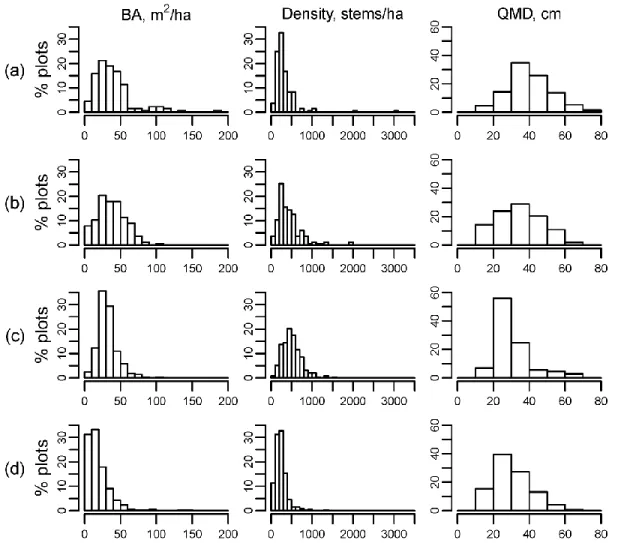
history data base ...45 1.3 Histograms (%) of plot BA, density, and QMD in the matched
datasets for (a) 1930s undisturbed plots; (b) 1990s–2000s undisturbed
plots; (c) 1990s–2000s disturbed plots; and (d) 1930s disturbed plots ...46 1.4 Mean (±SE) BA for each species functional group in each
time period, by disturbance history category ...47 2.1 Great Smoky Mountains National Park, North Carolina and
Tennessee, USA, with topographic relief and major forest types ...79 2.2 Location of six base stations used to monitor soil moisture
in GRSM between 2009 and 2011 ………...80 2.3 An example of typical wetting and drying curves for
soil moisture over time, for the Elkmont base station ...81 2.4 Regression of base station volumetric water content (VWC)
with a) gravimetric water content and b) VWC measurements
with the handheld time-domain reflectometry probe …….……...82 2.5 Illustration of the procedure for relativizing soil moisture
values (VWC) from point samples to base station values ..….…...…...83 2.6 Boxplot of 1995-2011 growing season precipitation from
meteorological stations associated with the base stations …………..…...84
3.1 Types of change in species response curves in response to
climate change or other drivers of change ……….…...……….……….135
3.2 Great Smoky Mountains National Park, North Carolina and
Tennessee, USA, with topographic relief and major forest types ..…….……....136
3.3 Disturbance history and fire in GRSM prior to park formation
3.4 Frequency of major disturbance history categories along
the elevation gradient in GRSM ………..…………...………138
3.5 Modeled 1930s distributions for 5 dominant tree species on
the elevation and moisture gradients in GRSM, before
near-complete (or ongoing) mortality from exotic pests ………139
3.6 Comparison of frequency distributions for 1930s and
1990s-2000s vegetation plots on the elevation and
landform index (LFI) gradients in GRSM ………..………140
3.7 Segment plot of Bayesian credible intervals for group-level
mean estimates (mu) of parameter x time interactions …………...………..141
3.8 Changes in modeled optima on the elevation and landform
index (LFI) gradients for 30 tree taxa between the 1930s
and 1990s-2000s ………..……….………..142
3.9 Boxplot of weediness index values by SDM
LIST OF ABBREVIATIONS
AIC Akaike information criterion
BA Basal area
CV Coefficient of variation dbh Diameter at breast height DEM Digital elevation model elev. Elevation
ETI Equal-tailed interval
Freq Frequency
GAM Generalized additive model GIS Geographic information system
GRSM Great Smoky Mountains National Park
ha Hectares
LFI Landform index
LiDAR Light detection and ranging LME Linear mixed effects
LMG Lindeman, Merenda, and Gold variance decomposition method PET Potential evapotranspiration
prob. probability of occurrence QMD Quadratic mean diameter RAD Solar radiation
Rep Reproduction
SDM Species distribution modeling SE Standard error
spp. Species (plural) Tasp Transformed aspect
TDR Time-domain reflectometry
Tol. Tolerance
TPI Topographic position index TSI Terrain shape index
TWI Topographic wetness index
UFRL Uplands Field Research Laboratory USDA U.S. Department of Agriculture USDI U.S. Department of the Interior VWC Volumetric water content
WI Weediness index
CHAPTER 1: STRUCTURAL AND COMPOSITIONAL CHANGE IN GREAT SMOKY MOUNTAINS NATIONAL PARK
SINCE PROTECTION, 1930s-2000s1
Introduction
Spatial and temporal variability in environment and disturbance, interacting with species adaptations, creates structural and compositional variability across forested landscapes. This variability has been shown to be important for the persistence of populations (both plants and wildlife), ecosystem function, and ecosystem services (Landres et al. 1999). With increased, pervasive anthropogenic impacts on forests and the need for effective management across
landscapes and regions, understanding and comparing historic and present-day range of variation in forest structure and composition serves important scientific, conservation, and management purposes. In eastern USA forests, previous studies of disturbance and forest structure have focused on single disturbance types (e.g., Clinton and Baker 2000), temporal sequences dating from specific disturbance events (e.g., Reilly et al. 2006), specific communities or site conditions (e.g., Jenkins et al. 2011), and restricted spatial scales (e.g., Elliott and Swank 1994). Research elsewhere has begun to focus on our critical need to understand the aggregate structural and compositional effects of multiple, widespread disturbances of different types across forested regions (Ohmann et al. 2007). To that end, in this chapter, we investigate the aggregate,
intensively used and managed.
Great Smoky Mountains National Park is the largest protected area in the Central Hardwood Region (CHR), encompassing a wide range of elevation and site conditions and harboring nearly the full range of southern Appalachian forest communities. The rugged topography, breadth of forest types, and high biodiversity in this region inspired its designation as a national park in 1934. While much of the park, like other areas in the southern
Appalachians, has a history of Native American land use (Grissino-Mayer 2016, Leigh 2016, Greenberg et al. 2016), European settlement, and logging, approximately 20 % of the park was free of direct human activities (i.e., logging, settlement, and herded livestock grazing) at the time of park creation. Since 1934, the entire park has been protected from further direct uses other than small areas used for recreation. Despite protection, however, multiple indirect, diffuse anthropogenic disturbances or changes in disturbance regime—including exotic pest
introductions, reduced fire frequency, atmospheric deposition, and changes in herbivory—have continued to impact nearly all GRSM forests. Fortunately, the National Park Service hired forester Frank Miller to conduct a park-wide vegetation survey in the 1930s; this detailed survey of forest structure and composition at the time of park formation provides a rare snapshot of landscape-level variation in forests both disturbed and undisturbed by humans. We expect the state of ‘undisturbed’ forests at that time to lie within the natural, historic range of variation for GRSM forest structure and composition, thereby representing an important reference for comparison to present-day forests. Likewise, areas impacted by pre-park human activities represent the initial conditions for forests that were subsequently protected from direct human use. We expect a comparison of present-day forests to these 1930s ‘bounding’ reference
forests after approximately 75 years of succession, and the effects of ongoing disturbances overlaid on both historically undisturbed and disturbed forests.
While no subsequent studies in GRSM (including Whittaker 1956) have been as
comprehensive as Miller’s survey (MacKenzie and White 1998), the combined wealth of middle to late twentieth century plot-level studies in GRSM—many of them efforts to understand and monitor forest dynamics with respect to disturbance—spans a range of park regions and environments (White and Busing 1993). Here, we compare a compilation of recent forest plot datasets to the Miller survey plots to assess differences in forest structure and composition, within and between time periods, with respect to disturbance history and dominant
environmental gradients. Specifically, we use maps of historic anthropogenic disturbance and terrain variables that represent temperature and moisture gradients to ask the following questions: (1) how do environment and disturbance history influence the distribution of basal area (BA), density, and relative species composition in each time period?; (2) what is the range of variation in BA, density, and average tree size, as measured by quadratic mean diameter (QMD) (Curtis and Marshall 2000), with respect to disturbance history in each time period?; and (3) how does the abundance of species functional groups, defined by species’ responses to disturbance and environment, differ across disturbance categories and time periods?
Study area
Physical Environment
decreases from 22 to 14 °C, and the mean January temperature decreases from 4 to −2 °C (Busing et al. 2005). Bedrock is primarily Precambrian metamorphosed sandstone, phyllite, schist, and shale, but one section is dominated by gneiss, granite, and schist, and there are small areas of limestone and related rocks. Soils are acidic and infertile and mostly consist of Ultisols and Inceptisols (USDA 2009).
Vegetation
The forest vegetation of GRSM is a complex of broad-leaved deciduous hardwoods and needle-leaved evergreen conifers (Jenkins 2007) controlled by environmental gradients, soil conditions, and disturbance (Figure 1.1) (Greenberg et al. 2016). At low elevations, community composition varies along a moisture gradient controlled by topography and soil characteristics, from diverse, mesic cove hardwood forests (on relatively higher pH soils) and less diverse Eastern hemlock (Tsuga canadensis, acid cove) forests (on lower pH soils) through oak
(Quercus)-dominated mid-slope positions to dry ridges dominated by yellow pine (Pinus
pungens, P. rigida, P. virginiana, P. echinata) and xerophytic hardwoods. The degree of pine
dominance on the ridges at any one time is likely controlled by fire history and outbreaks of the southern pine beetle (Dendroctonus frontalis) (Nowak et al. 2016). With increasing elevation, mesic cove hardwood and acid cove forests grade into northern hardwood forests and then, above about 1500 m in the central and eastern part of the park, into forests dominated by the needle-leaved evergreens red spruce (Picea rubens) and Fraser fir (Abies fraseri) and the
hardwood yellow birch (Betula alleghaniensis), with the occasional occurrence of high-elevation ‘beech gap’ (Fagus grandifolia) forests. At high elevations in the western part of the park, northern hardwoods dominate on north-facing and cooler landscape positions, with
American chestnut (Castanea dentata) was a frequent dominant or subdominant in all of these forests except for the highest elevation spruce-fir forests.
Natural disturbance
Both before and after federal protection in 1934, the landscape of GRSM experienced a wide variety of natural and anthropogenic disturbances, which collectively affected all parts of the landscape (Harmon et al. 1983). However, these disturbances varied widely in frequency, size, and magnitude. In this and the following section, we briefly review natural and
anthropogenic disturbances, with special reference to disturbances that cause tree mortality, thus causing structural and compositional variation and initiating successional dynamics, and those disturbances that can be mapped or otherwise quantified at the landscape scale.
disturbances have been studied at the stand scale but have not been mapped for GRSM at the landscape scale.
The second most important type of natural disturbance in the park is lightning-ignited fire and its interaction with mortality to mature pine caused by the southern pine beetle, a native insect (Barden and Woods 1976, Harmon 1982, Cohen et al. 2007, Flatley et al. 2013). Evidence of pre-park fires can be derived from fire scars (Harmon 1982, Flatley et al. 2013), charcoal (Welch 1999), and the structural and compositional characteristics of current stands (Harrod et al. 2000). However, understanding the spatial and temporal patterns of historical lightning fire in the park is complicated by centuries of overlay with pre-park fires set both by Native Americans and later European settlers (Barden and Woods 1976, Fowler and Konopik 2007). Since park establishment, lightning-ignited fires have exhibited a pattern of increasing frequency from wetter to drier sites along topographic gradients and decreasing frequency with elevation, particularly above 1,220 m (1940–1979) (Harmon 1981). These fires have tended to be warm-season fires (Harmon 1981, Cohen et al. 2007) and, unsuppressed, tend to burn over larger areas and for longer periods of time than suppressed fires (Cohen et al. 2007). Cohen et al. (2007) reported 140 lightning-ignited fires (128 suppressed, 12 unsuppressed) for GRSM between 1940 and 2006, or approximately 2.1 fires per year. Mean (±SE) annual number of lightning-ignited fires in the surrounding National Forests of the Blue Ridge Mountains ecoregion ranges from 2.0 ± 0.3 to 4.2 ± 0.7 per 2,000 km2 (1970–2013) (Greenberg et al. 2016).
Other natural disturbances are sometimes intense but are spatially less extensive. Ice storms are a phenomenon of middle to high elevations, usually causing damage to tree crowns and occasionally resulting in treefall (Lafon 2006, Butler et al. 2014, Lafon 2016). Like
high elevations and flood scour along stream channels. Debris slides occur where topography causes water to funnel into the steep headwaters of streams, and the sudden downslope fall of soils and vegetation leaves open bedrock behind (Clark 1987, Wooten 2016). Downstream, stormwater and flood-borne debris often scour the sides of the rocky stream channels (Leigh 2016). Debris slides and flood scour are intense but spatially restricted in the park landscape, affecting a very small percentage of park vegetation. Debris slides are documented in the park’s surficial geology map (USDA 2009), and effects of stream scour are documented indirectly in the GRSM vegetation classification (Madden et al. 2004) by yellow birch-dominated forests along streams.
Anthropogenic disturbance
Before European settlement of the southern Appalachians, Native American villages were located in major valleys and floodplains, and human activities on surrounding mountain slopes likely consisted of hunting and gathering on upper slopes and ridgetops as well as intentional use of fire in particular topographic settings (Delcourt and Delcourt 1997).
Concentrated European settlement occurred between the late 1700s and 1930 and was generally restricted to low-elevation (below 750 m), productive valley-flat sites and adjacent forest areas (Pyle 1988). Diffuse settlement and related human activities, such as early-style logging, gathering, livestock grazing, and use of low-intensity fire, extended to the areas surrounding concentrated settlement and were pervasive in the western end of the park (Pyle 1985). Livestock grazing, especially for the hard mast in the late summer and fall, occurred in pastures and forests around settlements. Livestock was also often taken to high-elevation summer pasture on grassy balds (Pyle 1985).
valuable species and sizes of trees (not the largest, not the smallest) (Pyle 1985). Logging companies soon began buying larger tracts of land, however, and built large logging camps and railroad lines, so that between about 1880 and 1930, corporate logging was a major disturbance to the park landscape, sometimes affecting entire watersheds and usually less selective in terms of species and tree sizes. Slash fires sometimes followed logging, and on some sites, these fires combined with soil erosion after rainstorms, causing delayed or absent regeneration of forests (some sites remain without a continuous forest cover 90 years after logging).
Park establishment ended the human-set fires of settlement and logging. The fire regime since 1934 has been dominated by arson and accidental fire with some lightning fire as well (Harmon 1981). However, reduction of human-set fires related to settlement and suppression of both human- and lightning-ignited fires has likely reduced fire frequency (Harmon 1982, Flatley et al. 2013) and extent (Cohen et al. 2007) in historically fire-maintained areas of the park.
Between 1940 and 1979, the mean (±SD) annual number of human-set fires in GRSM was 13.3 ± 10.02 (Harmon 1981). These fires tended to originate in more mesic areas and at lower
elevations than lightning-ignited fires during the same period, and human-set fire frequency peaked in April and November (Harmon 1981). Similarly, for 1930–2003, Flatley et al. (2011) found a mean (±SD) annual number of anthropogenic fires of 5.5 (4.9) per 1000 km2
(approximately half the area of the park). Although these fires may be more likely to originate in more mesic areas, Flatley et al. (2011) found no significant relationship between slope position and percent of total area burned. Mean (±SE) annual number of human-set fires in the
About 20 % of the park area has no history of direct anthropogenic disturbance (Pyle 1985, 1988). However, during the twentieth century, the remnants of undisturbed stands have been impacted by a wide range of human-mediated disturbances that have caused major canopy disturbance, including exotic pest introductions and air pollution (acid and nitrogen deposition, ozone). In terms of dominant tree cover, the effects of four exotic pest species have been
particularly dramatic: chestnut blight (Cryphonectria parasitica) (1920s to the present, with most dominant trees affected by the 1930s and dead by the 1950s) (Woods and Shanks 1959), balsam woolly adelgid (Adelges piceae) (1960s to the present, with most Fraser fir populations
drastically impacted by 1990) (Eagar 1984), beech bark disease (an insect-fungus disease complex initiated by Cryptococcus fagisuga) (late 1980s to the present, with high mortality of mature American beech trees) (Vandermast 2005, Taylor 2012), hemlock woolly adelgid
(Adelges tsugae) (early 2000s to the present) (Roberts et al. 2009, Onken and Reardon 2010,
Krapfl et al. 2011), and European wild boar (Sus scrofa) (rooting impacts concentrated in mesic forests and floodplains) (Bratton 1975). Air pollution mostly affects tree growth rates and not mortality (e.g., Johnson et al. 1992). Deposition of nitrogen and sulfur compounds through acid rain and fog increases with elevation and cloud exposure and therefore probably has greatest impact on forests of the highest elevations (Aneja et al. 1992). Air quality regulation greatly lowered sulfur deposition by the 1990s. Near-ground ozone exposure affects species susceptible to leaf damage, such as yellow buckeye (Aesculus flava) and black cherry (Prunus serotina) (Chappelka et al. 1999).
Data and methods
1930s forest plots
the park’s forest types. As the central focus of this effort, vegetation was sampled in 1378 plots in a grid across the entire park, although some watersheds were sampled more or less intensively than others. Some areas in the southwestern part of the park were not sampled because they were outside the proposed park boundary at that time. In each rectangular plot of 1 × 2 chains (20.12 m × 40.23 m), all live and dead trees greater than 4 in. (10.16 cm) in diameter at breast height (dbh) were identified to species, recorded as live or dead, and tallied in four size classes (converted to metric here): 10.16 to <30.48 cm, 30.48 to <60.96 cm, 60.96 to <91.44 cm, and ≥91.44 cm. Site environmental variables were recorded in the field, including but not limited to topographic variables such as elevation, slope steepness, and slope aspect. Surveyors noted whether or not plots had been burned or cut over, recording the known or estimated date of last burn or logging where possible. Plot locations were described on the data sheets, marked with an X on USGS topographic quadrangle maps, and later verified by Miller and his surveyors. In the 1980s, personnel at the Uplands Field Research Laboratory (UFRL) of GRSM digitized the plot data and transferred the plot locations by hand onto modern USGS topographic quadrangle maps. UFRL personnel annotated the digital dataset with calculations of live and dead BA (m2 per ha, based on geometric mean diameter for each size class) and density (stems per ha) for each species in each plot (see MacKenzie and White 1998 for further description of the Miller plot data). In 2004, Tuttle digitized the plot locations and, more recently, matched these locations to the plot data and performed extensive data cleaning, including assessing the accuracy of plot locations using the field data and GIS.
hierarchical divisive clustering method.
Busing et al. (1993) summarized the composition and structure of the northern hardwood—spruce-fir ecotone in the 1930s using a subset of the Miller plots. Although the Miller plots were not permanently marked, several studies have compared subsets of the Miller data to more recent, comparable plot samples to investigate change over time for specific
geographic regions, portions of environmental gradients, or forest types in GRSM (Walker 1978, Harrod 1999, Knebel 1999, Vandermast 2005, Tuttle 2007). Our study is the first to attempt a park-wide comparison of the Miller data to more recent datasets. Because we were interested in variation across types of disturbance, we selected all plots matched to a location and with at least one recorded tree ≥10 cm dbh for our study (1,284 plots). We excluded two plots that were extreme outliers in our initial analyses, yielding 1,282 plots for comparison. The Miller plot data reflect the standing-dead American chestnut trees on the landscape at that time; chestnut blight was in progress, but live American chestnut trees still dominated the landscape. In this study, we treated all standing-dead American chestnut trees as live, to obtain a better estimate of the true dominance of this species in historic GRSM forests. As a result, any early responses to chestnut blight that had begun may create some inflation of BA or density in our results. However, upon reviewing the history of the progression of chestnut blight in GRSM (Woods and Shanks 1959), we believe that any such initial responses would have minimal effect on our results.
The 1990s-2000s forest plots
we selected plots from the 1990s and 2000s to maximize time since the 1930s as well as
coverage across the park. Most datasets include field environmental data collected for each plot, including topographic variables such as elevation, slope steepness, and slope aspect. After data cleaning, including assessing the accuracy of plot locations using field data and GIS, we
developed a compilation of 490 plots for comparison to the Miller data. These plots occur in 17 out of 22 park watersheds, but the majority of plots are concentrated in three areas: the Abrams Creek watershed on the western end of the park, the Cataloochee Creek watershed on the southeastern end of the park, and the high-elevation spruce-fir zone in the central portion of the park. Most plot sizes in our compilation are 20 m × 50 m or 20 m × 40 m (similar in size to the Miller plots), with the exception of 20 m × 20 m plots in the spruce-fir zone and a few larger plots scattered elsewhere. We limited our compilation dataset to trees ≥10 cm dbh to match the Miller data, and we calculated BA (m2 per ha) and density (stems per ha) for each tree species in each plot.
Disturbance history and environment
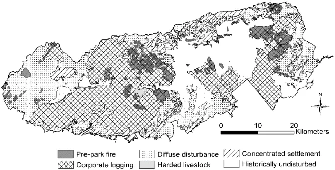
anthropogenic disturbance (hereafter referred to as undisturbed, although these plots would have been subject to natural disturbance). Pyle (1985) also compiled and mapped records of pre-park fire, largely consisting of post-logging slash fires but also areas with records or evidence of diffuse, smaller fires. Pyle’s compilation included evidence of cutting or fire recorded on the Miller plot data sheets and on Miller’s final park vegetation maps. Miller’s final vegetation maps show additional areas of cutting or burning not included in Pyle’s generalization. A GIS layer of disturbance history similar to Pyle’s maps exists in the GRSM geospatial database, but it differs from Pyle’s maps in important ways, and the layer is currently of unknown provenance. We scanned and georeferenced maps from Pyle (1985) and used both these maps and the digitized Miller maps as a guide to reclassify or modify polygons in the GIS disturbance history layer to match Pyle’s maps and categories (Figure 1.2). We combined several fire history datasets for GRSM into a GIS layer of all known, mapped areas of burn before park establishment (Figure 1.2), including evidence of prior burn from the 1930s plot data sheets, burned polygons from the digitized Miller vegetation map and the GRSM fire history layer, and burned areas from Pyle’s maps (Pyle 1985).
2005). These variables often overlap in their representations of microclimate and soil water balance and differ in the extent to which they isolate or integrate the effects of particular
microclimatic or hydrologic processes; as a result, terrain variables are often correlated, and sets of multiple, sometimes interacting terrain variables often best represent the aggregate
topographic effects on site conditions in vegetation models (e.g., Simon et al. 2005).
For this study, we assembled a set of terrain variables from a combination of field data and data layers developed by GRSM personnel and derived originally from a hybrid LiDAR- (primarily) and National Elevation Dataset-based, 3-m-resolution DEM. Terrain variables considered in our analyses include elevation; slope aspect, steepness, and curvature; potential annual solar radiation (RAD) (in watt-hours per m2); topographic wetness index (TWI) (Beven and Kirkby 1979, Moore et al. 1991); topographic position index (TPI) (Weiss 2001); terrain shape index (TSI) (McNab 1989, Bolstad et al. 1998); and landform index (LFI) (McNab 1993). Topographic wetness index represents relative moisture drainage at a site as a function of upslope contributing area (drainage input) and local slope steepness (drainage output); higher values of TWI imply greater relative moisture balance. Topographic position index represents relative slope position as the difference between a site’s elevation and the mean elevation of surrounding sites; negative values imply lower slope or valley-bottom positions, positive values imply upper slope or ridgetop positions, and values near zero imply flat or midslope positions. Terrain shape index represents local land surface shape (surface curvature gradient) as the mean slope gradient between the center of the plot and the plot boundary; low and high values
low values correspond to ridgetop positions that are not surrounded by higher ridges, and high values correspond to valley-bottom positions surrounded by steep slopes.
For slope steepness and aspect, we used values from field data where available. For missing field values and for all other terrain variables besides LFI, we extracted values for each plot location from 10-m (elevation) or 30-m (all others) spatial grids derived by GRSM
personnel from the original 3-m LiDAR DEM. We used the Whitebox Geospatial Analysis Tools software (Lindsay 2012) to derive LFI from the LiDAR-derived 30-m DEM. For several of these DEM-derived variables, values extracted from the 30-m layers performed better in our
preliminary analyses than 10-m values (where available or where separately derived by us). In addition, we reasoned that values derived from the fine-scale LiDAR DEM but rescaled or resampled to 30-m resolution more accurately represented average site conditions for the plot sizes in our dataset, most of which measured 20 m × 40 m or 20 m × 50 m. For LFI, the longer computation time for derivation from a 3-m or 10-m DEM was prohibitive and would have provided little benefit over the 30-m version for this variable based on watershed-level topography.
Data set matching
Because the 1990s–2000s plots were concentrated in three areas of the park and originated from different site selection strategies, differences in the spatial and topographic distributions of the two datasets could bias our comparisons. To avoid spurious comparisons, we used Optmatch, an optimal matching approach developed for comparative observational studies (Hansen and Klopfer 2006), to match the 1930s plots (‘controls’) to 1990s–2000s plots
vegetation studies in GRSM and preliminary statistical modeling of our datasets indicated that anthropogenic disturbance history, elevation, LFI, TPI, RAD, and park region were important predictors of forest structure and composition. We categorized the park into geographic regions similar in climatic, geologic, and topographic setting, approximately representing northwest, southwest, northeast, and southeast quadrants, with the highest elevations in the central and eastern part of the park combined as a single region. We then limited valid matches to plots within the same region, disturbance history category, elevation class (<600 m, 600–900 m, 900– 1,200 m, 1,200–1,600 m, and >1,600 m), and LFI class (<9.5, 9.5–16.5, and >16.5). We specified elevation (<100-m difference between plots), LFI, TPI, and RAD as matching criteria, selected Mahalanobis distance as the metric to optimize, and specified a matching ratio for number of 1930s plots matched to 1990s–2000s plots, to further exclude poor matches resulting from the large number of 1930s plots relative to the 1990s–2000s plots. A matching ratio of ≤3:1 produced the best combination of matching and sample size, yielding 529 plots from the 1930s and 460 plots from the 1990s–2000s for comparison. Box plots used to compare the distribution of the matched datasets on the continuous matching criteria (elevation, LFI, TPI, and RAD) indicated that the datasets were well matched within combinations of elevation and LFI classes (environmental/topographic ‘zip codes’) (Dean Urban pers. comm., Jobe 2006), with slight offsets of distribution for some variables in three infrequently sampled zip codes with low abundance on the landscape; low sample sizes did not permit further improvement of these matches.
Statistical modeling of structure and composition
disturbance history category, topography, and pre-park fire. Exploratory generalized additive models (GAM) of BA and density for each time period revealed that some predictors,
particularly elevation, exhibited a nonlinear relationship with BA or density; however, once significant interactions between predictors were taken into account, relationships with individual predictors were (approximately) linear, and we subsequently used linear regression. For
disturbance history categories, we chose to perform contrasts against the most disturbed category, which we hypothesized to be corporate logging, to highlight significant differences between disturbance categories that might not be apparent if all disturbance categories were contrasted against undisturbed. Model selection was guided by forward and backward stepwise selection by AIC. Because our models are not intended for prediction, we compared the final models in terms of overall variance explained as well as the identity, sign, and relative
importance of significant predictor variables. Relative importance for predictors in each model was calculated using the Lindeman, Merenda, and Gold (LMG) variance decomposition method available in the relaimpo package for R statistical software (Groemping 2007, R Core Team 2014).
location (mean) or dispersion (variance), we used betadisper in the Vegan package (Oksanen et al. 2013) to check for multivariate homogeneity of multivariate dispersion among groups in the datasets (Anderson 2006). This procedure confirmed that the significant predictors in our models reflected differences in location rather than dispersion. Differences in the overall drivers of forest composition between time periods were evaluated by comparing the final adonis models in terms of the identity and importance of significant predictor variables.
Comparisons of structure and functional composition by disturbance history
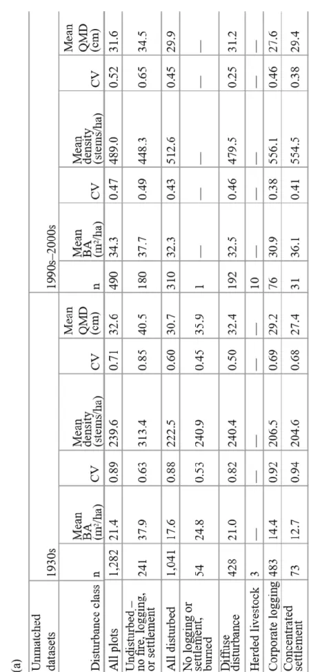
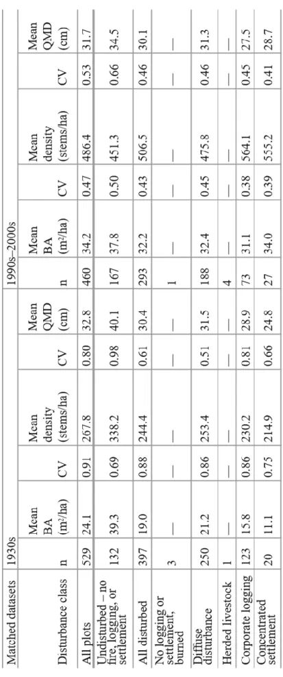
To determine the overall effects of pre-park and ongoing anthropogenic disturbance on forest structure, we calculated mean and coefficient of variation (CV) for BA, density, and QMD in each time period for the following groups: all plots, undisturbed plots, disturbed plots, and plots in each disturbance history category, excluding categories with sample size ≤10. We compared these metrics for unmatched and matched datasets to assess the effects of matching on results and interpretation. However, further analyses were based on comparison of the matched datasets to minimize the influence of regional and topographic biases in the 1990s–2000s dataset on our results. Histograms of BA, density, and QMD for disturbed and undisturbed subsets of the matched datasets were used to compare the landscape distribution of structural characteristics in these samples. Finally, we evaluated the effects of disturbance on functional composition by first categorizing species into functional groups (Table 1.1) and then plotting mean and standard error of BA for each functional group in each disturbance history category. Species were assigned to functional groups based on disturbance-related functional characteristics described in the
Results
Influence of disturbance history and environment on structure and composition
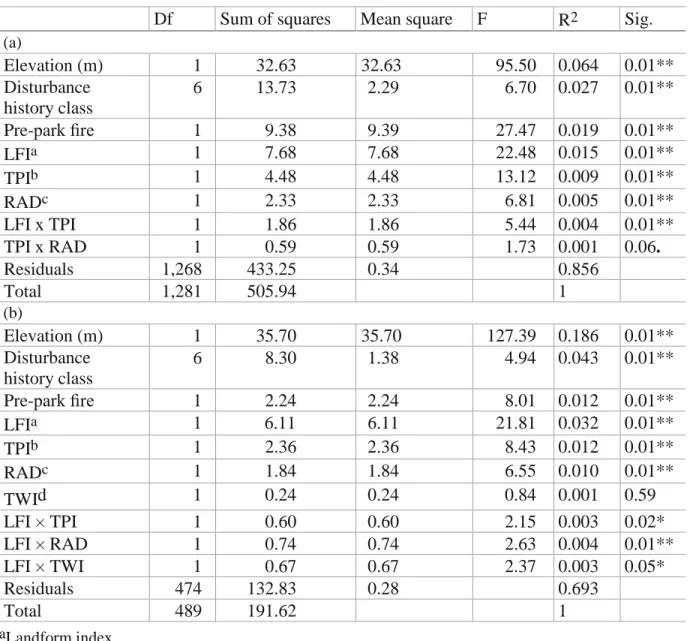
Topography, anthropogenic disturbance history, and pre-park fire explain between 12.6 % and 24.8 % (adjusted R2 11.5–24.3 %) of the variance in density and BA across the two time periods (Table 1.2). Different approaches for determining relative importance of regression predictors can yield different results, so the LMG variance decomposition results here should be interpreted with caution; however, our rankings according to LMG (Table 1.2) illustrate several interpretable changes in the variables that best explain how GRSM forests are structured.
Adonis models of compositional dissimilarity reveal differences between time periods similar to those for BA and density (Table 1.3). While disturbance categories and pre-park fire are significant predictors in both time periods, the relative importance of pre-park fire in
structuring composition decreases in the 1990s–2000s. Not surprisingly, elevation, the dominant environmental gradient in the park, is the most important predictor of composition for both time periods, and elevation more strongly determines the composition in the 1990s–2000s than in the 1930s. While disturbance category and fire are more important than individual topographic variables in the 1930s model, topographic variables emerge as equally important predictors in the 1990s–2000s model. Overall, the variance explained for compositional dissimilarity nearly doubles from the 1930s to the 1990s–2000s.
Effects of disturbance history on structural range of variation
Interestingly, the results for the matched datasets (Table 1.4b) are strikingly similar to the results with no matching (Table 1.4a), and we limit our discussion to results for the matched datasets (Table 1.4b). Mean BA for undisturbed plots shows little difference between the two time periods. In all disturbance categories, mean BA has increased from the 1930s to the 1990s– 2000s, approaching the value for undisturbed plots. The highly disturbed areas show the greatest increases in mean BA, nearly doubling for corporate logging and more than tripling for
cm for settlement. For undisturbed plots, mean QMD shows a notable decrease of 5.6 cm.
Combining these structural characteristics yields four structural groups with, on average: (1) high BA, moderate density, and high QMD (1930s undisturbed); (2) low BA, low density, and low QMD (1930s disturbed); (3) high BA, high density, and moderate QMD (1990s–2000s undisturbed); and (4) moderate BA, high density, and low QMD (1990s–2000s disturbed). Variation around mean BA and density, as represented by CV, shows marked differences across time periods and between disturbed and undisturbed categories (Table 1.4b). These differences are best understood by examining histograms of plot BA, density, and QMD for disturbed and undisturbed categories in each time period (Figure 1.3). Basal area for 1930s undisturbed plots (Figure 1.3a) exhibits a broad peak in the 10–60 m2 per ha range with few plots <10 m2 per ha and positive skew with a long tail of high-BA plots, up to nearly 190 m2 per ha. The 1930s undisturbed density distribution (Figure 1.3a) exhibits a narrow peak between 100 and 300 stems per ha with few plots <100 stems per ha and again positively skewed with scattered high-density plots up to nearly 3,100 stems per ha. The moderate and high CV for BA and density,
respectively, reflects the scale, location, and positive skew of these distributions. Quadratic mean diameter for 1930s undisturbed plots (Figure 1.3a) shows a unimodal, nearly symmetric
For disturbed plots, the 1930s distributions exhibit narrow peaks of BA and density concentrated in the lowest classes and very few extreme high values; QMD is likewise positively skewed with a low mean (Figure 1.3d). Of note, the 1930s disturbed density distribution is similar to the 1930s undisturbed distribution, although with a narrower peak that is more concentrated at lower densities; however, the strikingly different BA and QMD distributions paired with these similar density distributions sharply differentiate the two categories. In comparison to the 1930s disturbed plots, the 1990s–2000s disturbed BA distribution (Figure 1.3c) exhibits a shift to a higher mean, and the BA peak remains narrow with positive skew. The density distribution has shifted to a broad peak at a higher mean that surpasses the 1930s
undisturbed mean. The QMD distribution shows no change in mean from the 1930s and marked narrowing of the peak, with reductions in frequency of both low- and high-QMD plots.
Effects of disturbance history on functional composition
Mean BA is low for all species groups across the disturbed categories and for several species groups at their elevational limits in the predominantly high-elevation undisturbed
category (Figure 1.4). American chestnut still dominated the 1930s landscape (although much of it was already standing dead); mean BA for this single species was comparable to mean BA for functional groups made up of several species. In contrast, American chestnut is essentially absent from all categories in the 1990s–2000s dataset. In the undisturbed category, all species groups other than American chestnut exhibit no significant difference in mean BA.
dominant or codominant in settlement and diffuse disturbance areas. Moderate disturbance responders increased and became a dominant species group in corporate logging areas. Average increases of this group in diffuse disturbance and settlement areas are moderate to low compared to increases for other species groups. Oaks as a group did not decrease in any category and increased significantly in diffuse disturbance and settlement areas. Slow-growing, drought-tolerant species dominated by hickory (Carya) species did increase in areas of diffuse disturbance and settlement but were of low mean BA and relatively unimportant for overall compositional change. As a group, yellow pine species did not decrease in mean BA in any category and exhibited a large, significant increase in settlement areas.
Discussion
Overlays of disturbance and environment
Sampling variability and variables not included in our analysis likely contribute to the low proportion of variance explained by the models and also complicate interpretation of model results. In terms of sampling variability, forests with similar environment and history will show variation at the scale of the plots (0.04–0.1 ha) used here. In old growth mesic
hemlock-hardwood forests, Busing and White (1993) showed that CV of total BA and density was dependent on plot size, decreasing to 10–15 % of means only at plot scales of 0.5 ha, and
Whittaker (1966) found similar values for CV in old growth spruce-fir forests at the 0.5 ha scale. Coefficient of variation in forests dominated by smaller trees and those that are even-aged (owing to stand initiating disturbances) would decrease to 10–15 % at plot sizes smaller than 0.5 ha, but it is likely that a substantial proportion of the unexplained variation in our results reflects expected variability among plots for the plot sizes in our samples.
disturbance history at plot locations, time since pre-park anthropogenic disturbance, post-park fires, the discrete locations and types of disturbance in areas mapped as diffuse disturbance, and, for the 1990s–2000s models, unmapped post-park disturbances such as the decimation of
American chestnut, American beech, and Fraser fir. In addition, the distribution of unmapped disturbances and unquantified severities is likely correlated with elevation and topography. For instance, the increase of BA and density with elevation in the 1930s may represent a range of factors, such as lower levels of diffuse disturbance at higher elevations or the correlation of most major disturbances with low elevation, rather than a true environmental gradient. Likewise, site topographic variables like LFI and TPI (and their interactions) as predictors of 1930s BA and density may represent unmapped variation in degree of disturbance from cove to ridge, such as preferential siting of agricultural fields and grazing areas or logging limited to accessible topographic positions or desirable forest types. Elevation and topography, particularly LFI, are relatively more important predictors of BA and density for the 1990s–2000s dataset compared to the 1930s dataset; once again, however, site topographic variables are likely correlated with such factors as fire suppression and the distribution and timeline of disturbance by exotic pests (via the niches of both the pests and host species). Nevertheless, the decreased importance of anthropogenic disturbance history (including human-set fires) combined with the increased importance of elevation and topography across the models for BA, density, and compositional dissimilarity indicates sorting of structure, species, and forest communities along environmental and disturbance gradients during 60–75 years of response to historic and recent disturbances.
In summary, a complicating factor in understanding the relative roles of disturbance and environment is that natural and anthropogenic disturbances are not independent of the
recovery times. Further, natural and historic anthropogenic disturbances overlap in spatial distribution in GRSM but differ in timing, severity, and extent. For instance, catastrophic disturbances such as clear-cut logging in the high elevations (removal of the canopy over large areas), are inverse to the pattern of natural disturbance (low rates of canopy turnover through small gaps). Patterns of post-park anthropogenic disturbances further differ from historical disturbances. For instance, while decimation of American chestnut, Fraser fir, and American beech may follow environmental gradients related to niches of the host and pest species, these canopy disturbances have been widespread but diffuse (compared to widespread and intense logging) and have occurred over a relatively short time period (compared to natural-disturbance-related gap formation). The combined effects of widespread, major anthropogenic disturbances, particularly when multiple such disturbances occur on a relatively short time scale (within the same century or a few decades), can mask environmental gradients, including patterns along those gradients that were also shaped by natural disturbances.
Overlays of disturbance before and after park establishment
interpreted with some caution, because some sampling biases and differences in environmental distribution that were not corrected by our plot matching method could be generating over- or underestimates of difference between our matched values. Specifically, the 1990s–2000s undisturbed plots were biased toward the highest elevations (≥1,600 m), while the 1930s plots were biased toward plots between 1,200 and 1,600 m elevation. Sampling bias in the design of several 1990s–2000s studies (toward plots containing Eastern hemlock), particularly in the 1,200–1,600 m range, likely biased our comparison toward higher 1990s–2000s mean BA; at the same time, the disproportionate number of 1990s–2000s plots ≥1,600 m likely biased our
comparison to lower 1990s–2000s mean BA (from Fraser fir decline). Improved plot matching aimed at similar proportions of elevation and topographic settings across time periods would decrease the number of plots for comparison but could increase confidence in the aggregate differences between time periods.
We expected the 1990s–2000s disturbed distributions, in the absence of continued major disturbance, to show recovery over approximately 75 years of succession. While BA in
back toward lower QMD.
While we might use the 1930s undisturbed histograms as a reference for the 1990s–2000s undisturbed plots, their use as a reference for the 1990s–2000s disturbed plot distributions may be limited because of the paucity of known undisturbed plots in the park’s lower elevations, where disturbed plots are concentrated. Spatial and environmental matching of disturbed to undisturbed plots (where enough plots are available) would be necessary to make comparisons that account for differences in natural disturbance regimes (particularly fire) and species’ characteristics along elevation and topographic gradients. Future examination of the diffuse disturbance plots alone might be instructive, in comparison to other disturbed and undisturbed plots (where enough matching plots are available). Even though the frequency and character of human-set fires might have differed from the natural fire regime and levels of forest clearing might not be characteristic of any natural disturbances in GRSM, the diffuse nature of the disturbances appears to have generated an aggregate effect on structure intermediate to areas of more major disturbance (logging and settlement) and undisturbed areas. In addition, Pyle (1985) mapped areas of diffuse disturbance with ‘big trees,’ indicating even lower levels of diffuse disturbance in some areas. Such comparison could also help us better understand the effects of diffuse human activities on the landscape.
landscapes, likely indicates that other shade-tolerant species increased in response to decreases caused by exotic pests. Tuttle (2007) found that red spruce, understory maples (Acer
pensylvanicum, A. spicatum), and yellow birch all increased in the northern hardwood –
spruce-fir ecotone in conjunction with decline of Fraser spruce-fir. However, yellow birch’s species group (moderate disturbance responders) does not show increases in mean BA for the undisturbed category. In addition, both Fraser fir and American beech respond rapidly to disturbance in stands where they dominate, with abundant regeneration (Fraser fir) (Smith and Nicholas 2000) or vigorous sprouting (American beech) (Vandermast 2005). American mountain ash (Sorbus
americana) and pin cherry (Prunus pensylvanica), both vigorous disturbance responders,
increased in undisturbed areas in response to Fraser fir decline (Busing et al. 1988, Tuttle 2007), but these trees do not dominate stand BA, are short-lived, and may have already peaked in disturbance response. As for the structural comparisons, these aggregate compositional
comparisons for undisturbed areas should be interpreted with some caution because of sampling and environmental biases between the matched plots. For instance, the possible bias of the 1990s–2000s plots toward more Eastern hemlock and more Fraser fir could have resulted in an overestimate of mean BA in the shade-tolerant species group.
Dramatic increases in vigorous disturbance responders in all disturbed categories reflect primarily dramatic increases in both red maple (A. rubrum) and yellow-poplar (Liriodendron
tulipifera) as well as large increases in Eastern white pine (Pinus strobus). All three of these
species are long-lived enough to persist in the landscape in the absence of further major
supports observations that yellow-poplar attains high BA rapidly and dominates the canopy in many former settlement areas, suppressing canopy attainment by other species, particularly shade-tolerant species. The increase in the yellow pine group in settlement areas like reflects early-successional dominance of Virginia pine in some old fields. However, the similar mean BA of both oaks and shade-tolerant species in this category may indicate that the relatively short-lived Virginia pine stands are declining, and slower-growing species are increasing.
The clustering of different species groups in the diffuse disturbance category in the 1990s–2000s dataset may reflect the diffuse, patchy nature of the disturbances as well as the variety of topographic settings in this category that covers large portions of the GRSM landscape at low and middle elevations. With a range of pre-park disturbance types, sizes, and ages, species across all groups will respond somewhere, according to their adaptations for regeneration or recovery from disturbance. Increases in this category are also likely driven by both the decline of American chestnut and decrease in fire frequency and extent, particularly with fire suppression and the removal of frequent burning by humans in the western part of the park (Pyle 1985). Although mean BA did not decrease for the yellow pine group in this category, this result cannot distinguish between the effects of any post-park fires in maintaining yellow pine stands (less likely) or in-fill of other species where pines persist but fire is absent (more likely); clearly, the fire- and dry-site-adapted yellow pines are not abundant responders to landscape recovery from diffuse pre-park disturbances, nor to continued disturbances such as chestnut blight.
The corporate logging category spans a wide range of elevation, topographic settings, and times since disturbance; as a result, it is not surprising that a variety of species groups,
may reflect recovery of conifers and mesic hardwoods in more mesic and higher-elevation logged areas, the secondary dominance of the two disturbance-responder groups in this category is indicative of response to widespread clear-cutting and, likely, to later disturbances such as chestnut blight, balsam woolly adelgid, and beech bark disease. Perhaps future analysis of co-occurring species in each time period as well as comparison of diffuse disturbance and corporate logging plots to undisturbed plots that overlap in elevation and topography (where enough
matched plots are available) could help disentangle the mix of responses to different disturbances and their relationship with undisturbed reference conditions.
Differences in Eastern hemlock abundance between the 1930s and 1990s–2000s datasets are worthy of separate discussion. Much of the increase in the shade-tolerant species group across disturbed categories is accounted for by increases in Eastern hemlock mean BA (not shown). Eastern hemlock seems to have broadly responded with recovery and/or increases in response to disturbance, likely including increases from chestnut blight on more mesic sites (as observed in Woods and Shanks 1959) and some increases on slopes with reduced fire frequency. It is possible, too, that much Eastern hemlock was left on the landscape by settlers and some selective logging operations (Pyle 1985), fostering its increase after disturbance. Some of the apparent increase in this study could be an artifact of biased sampling in our 1990s–2000s compilation. However, Tuttle and White (2011) found that Eastern hemlock increased in relative frequency on the GRSM landscape from 19.26 to 25.78 % between the 1930s and 1999.
the widespread Eastern hemlock trees in GRSM over the last several years represents yet another landscape-level set of canopy disturbances that will further distort the range of variation in these forests, even if recent treatment successes with Eastern hemlock continue.
Conclusions
Our results illustrate the ways that anthropogenic disturbances can both mask and interact with environmental gradients to structure CHR and temperate forests. After several decades of succession from widespread, major disturbance in all but approximately 20 % of GRSM,
historical anthropogenic disturbance has remained important as a predictor of forest structure and composition, although its importance has decreased relative to topography, and the level of importance differs with type of disturbance. The increased importance of topography implies sorting of structure and composition along environmental gradients. However, historical
disturbances and more recent anthropogenic disturbances interact with topography and differ in pattern on the landscape, complicating attempts to understand how environmental gradients contribute to forest structure and composition across the region.
Re-sampled plots and consistent coverage of plots across the landscape would have improved our modeling and comparisons. Miller’s survey plots were not permanently marked, making resampling and direct comparison impossible. More modern research projects have tended to be designed around immediate management problems limited to particular portions of the landscape and, as a result, have not provided consistent coverage of plots across the
landscape. To disentangle the aggregate effects of anthropogenic disturbance, natural
that does not rely on topographic approximations of environment. We also need more specific, detailed maps (or models) of historic and recent disturbances, including the timeline, extent, and intensity of these events. Additional digitization and spatial referencing of historical disturbance records as well as increased field data collection and mapping with remote sensing tools, such as LiDAR, could improve our efforts going forward. These needs are even more pronounced on managed and private lands, where management activities and land use further complicate the picture.
hemlock trees in GRSM from the hemlock woolly adelgid is not included our 1990s–2000s dataset, so further changes in structure beyond those observed in our results have already occurred.
Structural diversity and disturbance are keys to maintaining the habitats on which biodiversity depends. Reintroduction of fire is important for maintaining structural diversity and persistence of fire-maintained species in landscapes historically structured by a natural fire regime. However, in forests not historically structured by fire, impeded succession and the ongoing, rapid loss of remaining old-growth forests historically structured by small canopy gaps—and the loss of the largest trees from these forests—are concerning. A long series of exotic pest species has altered structure and composition of eastern USA forests, and additional species are likely to invade, underscoring the importance of efforts to minimize further impacts and to develop management approaches that will allow the redevelopment of stand and
landscape-level structural complexity consistent with old-growth forests (Franklin et al. 2002). While the pace of climate change in this region has been slow, future climate change will further affect GRSM and other CHR forests. The broad extent and significant complexity of ongoing and impending disturbances highlight the need for region-wide assessment of the aggregate effects of multiple stressors across protected, managed, and private lands.
Acknowledgments
ENDNOTE
REFERENCES
Anderson, M. J. 2001. A new method for non-parametric multivariate analysis of variance. Austral Ecology 26:32–46.
Anderson, M. J. 2006. Distance-based tests for homogeneity of multivariate dispersions. Biometrics 62:245–253.
Aneja, V. P., W. P. Robarge, C. S. Claiborne, A. Murthy, D. Soo-Kim, D., and Z. Li. 1992. Chemical climatology of high elevation spruce-fir forests in the southern Appalachian Mountains. Environmental Pollution 75:89–96.
Barden, L. S., and F. W. Woods. 1976. Effects of fire on pine and pine-hardwood forests in the southern Appalachians. Forest Science 22:399–403.
Beven, K. J., and M. J. Kirkby. 1979. A physically based, variable contributing area model of basin hydrology. Hydrological Sciences Bulletin 24:43–69.
Bolstad, P. V., W. Swank, and J. Vose. 1998. Predicting southern Appalachian overstory vegetation with digital terrain data. Landscape Ecology 13:271–283.
Bratton, S. P. 1975. The effect of the European wild boar, Sus scrofa, on gray beech forest in the Great Smoky Mountains. Ecology 56:1356–1366.
Burns, R. M., and B. H. Honkala, technical coordinators. 1990. Silvics of North America: 1. Conifers; 2. Hardwoods. Agriculture handbook 654. USDA Forest Service, Washington, DC, USA.
Busing, R. T. 1993. Three decades of change at Albright Grove, Tennessee. Castanea 58:231– 242.
Busing, R. T., and P. S. White. 1993. Effects of area on old-growth forest attributes: Implications for the equilibrium landscape concept. Landscape Ecology 8:119–126.
Busing, R. T., E. E. C. Clebsch, C. C. Eagar, and E. F. Pauley. 1988. Two decades of change in a Great Smoky Mountains spruce-fir forest. Bulletin of the Torrey Botanical Club 115:25– 31.
Busing, R. T., E. E. C. Clebsch, and P. S. White. 1993. Biomass and production of southern Appalachian cove forests reexamined. Canadian Journal of Forest Research 23:760–765. Busing, R. T., L. A. Stephens, and E. E. C. Clebsch. 2005. Climate data by elevation in the Great
Butler, S. M., A. S. White, K. J. Elliott, and R. S. Seymour. 2014. Disturbance history and stand dynamics in secondary and old-growth forests of the southern Appalachian Mountains, USA. Journal of the Torrey Botanical Society 141:189–204.
Chappelka, A., G. Somers, and J. Renfro. 1999. Visible ozone injury on forest trees in Great Smoky Mountains National Park, USA. Water Air and Soil Pollution 116:255–260. Clark, G. M. 1987. Debris slide and debris flow historical events in the Appalachians south of the
glacial border. Pages 125-137 in J. E. Costa and G. F. Wieczorek, editors. Debris
flows/avalanches: process, recognition, and mitigation. Reviews in Engineering Geology 7. Geological Society of America, Boulder, Colorado, USA.
Clinton, B. D., and C. R. Baker. 2000. Catastrophic windthrow in the southern Appalachians: characteristics of pits and mounds and initial vegetation responses. Forest Ecology and Management 126:51–60.
Cohen, D., B. Dellinger, R. Klein, and B. Buchanan. 2007. Patterns in lightning-caused fires at Great Smoky Mountains National Park. Fire Ecology 3:68–82.
Curtis, R. O., and D. D. Marshall. 2000. Why quadratic mean diameter? Western Journal of Applied Forestry 15:137–139.
Delcourt, H. R., and P. A. Delcourt. 1997. Pre-Columbian Native American use of fire on southern Appalachian landscapes. Conservation Biology 11:1010–1014.
Eagar, C. C. 1984. Review of the biology and ecology of the balsam woolly aphid in southern Appalachian spruce-fir forests. Pages 36-50 in P. S. White, editor. The southern Appalachian spruce-fir ecosystem: its threats and biology. Research/resources
management report SER-71. USDI National Park Service Southeast Regional Office, Atlanta, Georgia, USA.
Elliott, K. J., and W. T. Swank. 1994. Impacts of drought on tree mortality and growth in a mixed hardwood forest. Journal of Vegetation Science 5:229–236.
Flatley, W. T., C. W. Lafon, C. W., and H. D. Grissino-Mayer. 2011. Climatic and topographic controls on patterns of fire in the southern and central Appalachian Mountains, USA. Landscape Ecology 26 195–209.
Flatley, W. T., C. W. Lafon, H. D. Grissino-Mayer, and L. B. LaForest. 2013. Fire history related to climate and land use in three southern Appalachian landscapes in the eastern United States. Ecological Applications 23:1250–1266.
Fowler, C., and E. Konopik. 2007. The history of fire in the southern United States. Human Ecology Review 14:165–176.