Algorithms for Trust-Region Subproblems with
Linear Inequality Constraints
Melanie L. Bain Gratton
A dissertation submitted to the faculty of the University of North Carolina at Chapel Hill in partial fulfillment of the requirements for the degree of Doctor of Philosophy in the Department of Statistics and Operations Research.
Chapel Hill 2012
Approved by:
Jon W. Tolle
Gabor Pataki
Shu Lu
Scott Provan
c
2012
Abstract
MELANIE L. BAIN GRATTON: Algorithms for Trust-Region Subproblems with Linear Inequality Constraints.
(Under the direction of Jon W. Tolle.)
In the trust-region framework for optimizing a general nonlinear function subject to
nonlinear inequality constraints, sequential quadratic programming (SQP) techniques
generate subproblems in which a quadratic function must be minimized over a spherical
region subject to linear inequality constraints. An interior-point algorithm proposed
by Kearsley approximately solves these subproblems when the objective functions are
large-scale and convex. Kearsley’s algorithm handles the inequality constraints with a
classical log-barrier function, minimizing quadratic models of the log-barrier function
for fixed values of the barrier parameter subject to the trust-region constraint. Kearsley
recommends the LSTRS algorithm of Rojas et al. for minimizing these models. For
the convex case, we prove convergence of Kearsley’s algorithm and suggest alternatives
to the LSTRS algorithm. These alternatives include the new annulus algorithm of
Griffin et al., which blends the conjugate gradient and sequential subspace minimization
methods to yield promising numerical results. For the nonconvex case, we propose and
test a new interior-point algorithm that incorporates the annulus algorithm into an
SQP framework with trust regions.
Acknowledgments
I would like to express my gratitude to my advisor, Jon W. Tolle, for taking on just
one more graduate student. I could not have made it this far without his support and
guidance (and patience – LOTS of patience). I would also like to thank my committee
members G´abor Pataki, Shu Lu, Scott Provan, and Douglas Kelly for their feedback and
advice. I am very grateful to Joshua Griffin and Wenwen Zhou of SAS Institute, who
made great suggestions and always gave generously of their time when I had questions.
I would like to thank my parents Eileen and Robert, my uncle Ron, my Mamaw,
and my siblings Timothy, Christina, Ryan, and Kathleen for their love and support.
I would like to thank the UNC Board of Governors, the Statistical and Applied
Mathematical Sciences Institute, the Department of Statistics and Operations Research
at UNC, and SAS Institute for providing me with employment and learning
opportu-nities. Many thanks to Gehan Corea, Manoj Chari, and Radhika Kulkarni of SAS for
helping me to refine my skills and find my confidence.
I would like to thank all the faculty and staff who contributed to my education,
especially the professors and staff in the UNC STOR department, for their hard work
and dedication.
Finally, I’d like to thank all the amazing friends, extended family, and coworkers
who have enriched my life over the years. I am particularly grateful to Aaron Jackson
and Kevin Kesseler for helping me through the toughest times.
Thank you all.
Table of Contents
Abstract . . . iii
List of Figures . . . ix
1 Introduction . . . 1
1.1 General Problem . . . 1
1.2 Line-search and Trust-region Approaches . . . 2
1.3 Sequential Quadratic Programming . . . 5
1.3.1 Merit Functions and Filters . . . 6
1.4 Penalty Function Methods . . . 7
1.5 Large-scale Problems . . . 7
1.6 Problem of Interest . . . 8
1.7 Outline . . . 9
2 Analysis of Trust-region Subproblems . . . 10
2.1 Necessary and Sufficient Conditions . . . 10
2.2 Properties of the Parameterized Solution . . . 13
2.2.1 Case 1 . . . 18
2.2.2 Case 2 . . . 18
2.2.3 Case 3 . . . 19
2.2.4 Case 4 . . . 22
3 Algorithms for Trust-region Subproblems . . . 24
3.1 Small-scale Case . . . 24
3.1.1 Positive Definite H . . . 24
3.1.2 IndefiniteH . . . 25
3.2 Large-scale Case . . . 31
3.2.1 Conjugate Gradient Methods . . . 31
3.2.2 Lanczos Methods . . . 33
4 Algorithms for Inequality-constrained Trust-region Subproblems . 49 4.1 Convex Case: Kearsley . . . 49
4.1.1 Convergence of Minor Iterations . . . 52
4.1.2 Potential Hard Case . . . 58
4.1.3 Observations . . . 60
4.2 Nonconvex Case . . . 60
4.2.1 Proposed Algorithm . . . 60
5 Numerical Results . . . 71
5.1 Positive Definite Problems . . . 72
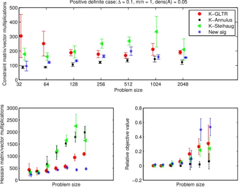
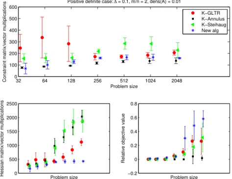
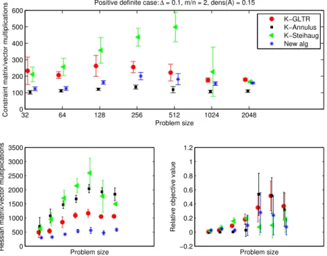
5.1.1 Observations . . . 73
5.2 Indefinite Problems . . . 76
5.2.1 Observations . . . 76
6 Conclusions and Future Work . . . 79
6.1 Future Work . . . 79
A Details of Basic Algorithms . . . 81
A.1 Conjugate Gradient Algorithm . . . 81
A.2 Lanczos Algorithm . . . 81
B Full Results of Numerical Tests . . . 84
B.1 Positive Definite Case . . . 84
B.2 Indefinite Case . . . 98
List of Figures
1.1 Line-search and trust-region steps . . . 4
2.1 Case 1, second subcase; Case 2 . . . 19
2.2 Case 3, second subcase . . . 20
2.3 Case 3, third subcase (the hard case) . . . 21
3.1 Φ(λ) with kxNk>∆, hard case not in effect . . . . 28
3.2 Φ(λ) with kxNk=kx(0)k<∆, hard case not in effect . . . . 28
3.3 Φ(λ), hard case in effect . . . 29
3.4 Annulus algorithm: restart indicated . . . 46
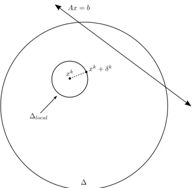
4.1 Proposed algorithm: local trust region centered at xk . . . . 63
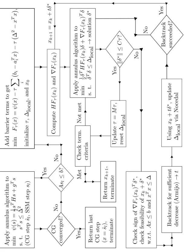
4.2 Flowchart for proposed algorithm . . . 70
5.1 Positive definite H, ∆ = 0.1,m =n, density of A= 0.05 . . . 73
5.2 Positive definite H, ∆ = 1, m=n, density of A= 0.15 . . . 74
5.3 Positive definite H, ∆ = 10, m = 2n, density of A= 0.05 . . . 75
5.4 Indefinite H, ∆ = 0.1,m= 0.5n, density of A= 0.05 . . . 76
5.5 Indefinite H, ∆ = 1,m = 0.5n, density of A= 0.05 . . . 77
5.6 Indefinite H, ∆ = 10, m =n, density of A= 0.15 . . . 78
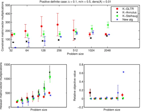
B.1 Positive definite H, ∆ = 0.1,m = 0.5n, density of A = 0.01 . . . 84
B.2 Positive definite H, ∆ = 0.1,m = 0.5n, density of A = 0.05 . . . 85
B.3 Positive definite H, ∆ = 0.1,m = 0.5n, density of A = 0.15 . . . 85
B.4 Positive definite H, ∆ = 0.1,m =n, density of A= 0.01 . . . 86
B.5 Positive definite H, ∆ = 0.1,m =n, density of A= 0.05 . . . 86
B.6 Positive definite H, ∆ = 0.1,m =n, density of A= 0.15 . . . 87
B.7 Positive definite H, ∆ = 0.1,m = 2n, density of A= 0.01 . . . 87
B.8 Positive definite H, ∆ = 0.1,m = 2n, density of A= 0.05 . . . 88
B.9 Positive definite H, ∆ = 0.1,m = 2n, density of A= 0.15 . . . 88
B.10 Positive definite H, ∆ = 1, m= 0.5n, density of A= 0.01 . . . 89
B.11 Positive definite H, ∆ = 1, m= 0.5n, density of A= 0.05 . . . 89
B.12 Positive definite H, ∆ = 1, m= 0.5n, density of A= 0.15 . . . 90
B.13 Positive definite H, ∆ = 1, m=n, density of A= 0.01 . . . 90
B.14 Positive definite H, ∆ = 1, m=n, density of A= 0.05 . . . 91
B.15 Positive definite H, ∆ = 1, m=n, density of A= 0.15 . . . 91
B.16 Positive definite H, ∆ = 1, m= 2n, density of A= 0.01 . . . 92
B.17 Positive definite H, ∆ = 1, m= 2n, density of A= 0.05 . . . 92
B.18 Positive definite H, ∆ = 1, m= 2n, density of A= 0.15 . . . 93
B.19 Positive definite H, ∆ = 10, m = 0.5n, density of A = 0.01 . . . 93
B.20 Positive definite H, ∆ = 10, m = 0.5n, density of A = 0.05 . . . 94
B.21 Positive definite H, ∆ = 10, m = 0.5n, density of A = 0.15 . . . 94
B.22 Positive definite H, ∆ = 10, m =n, density of A= 0.01 . . . 95
B.23 Positive definite H, ∆ = 10, m =n, density of A= 0.05 . . . 95
B.24 Positive definite H, ∆ = 10, m =n, density of A= 0.15 . . . 96
B.25 Positive definite H, ∆ = 10, m = 2n, density of A= 0.01 . . . 96
B.26 Positive definite H, ∆ = 10, m = 2n, density of A= 0.05 . . . 97
B.27 Positive definite H, ∆ = 10, m = 2n, density of A= 0.15 . . . 97
B.28 Indefinite H, ∆ = 0.1,m= 0.5n, density of A= 0.01 . . . 98
B.29 Indefinite H, ∆ = 0.1,m= 0.5n, density of A= 0.05 . . . 99
B.30 Indefinite H, ∆ = 0.1,m= 0.5n, density of A= 0.15 . . . 99
B.32 Indefinite H, ∆ = 0.1,m=n, density of A= 0.05 . . . 100
B.33 Indefinite H, ∆ = 0.1,m=n, density of A= 0.15 . . . 101
B.34 Indefinite H, ∆ = 0.1,m= 2n, density of A= 0.01 . . . 101
B.35 Indefinite H, ∆ = 0.1,m= 2n, density of A= 0.05 . . . 102
B.36 Indefinite H, ∆ = 0.1,m= 2n, density of A= 0.15 . . . 102
B.37 Indefinite H, ∆ = 1,m = 0.5n, density of A= 0.01 . . . 103
B.38 Indefinite H, ∆ = 1,m = 0.5n, density of A= 0.05 . . . 103
B.39 Indefinite H, ∆ = 1,m = 0.5n, density of A= 0.15 . . . 104
B.40 Indefinite H, ∆ = 1,m =n, density of A= 0.01 . . . 104
B.41 Indefinite H, ∆ = 1,m =n, density of A= 0.05 . . . 105
B.42 Indefinite H, ∆ = 1,m =n, density of A= 0.15 . . . 105
B.43 Indefinite H, ∆ = 1,m = 2n, density of A= 0.01 . . . 106
B.44 Indefinite H, ∆ = 1,m = 2n, density of A= 0.05 . . . 106
B.45 Indefinite H, ∆ = 1,m = 2n, density of A= 0.15 . . . 107
B.46 Indefinite H, ∆ = 10, m = 0.5n, density of A = 0.01 . . . 107
B.47 Indefinite H, ∆ = 10, m = 0.5n, density of A = 0.05 . . . 108
B.48 Indefinite H, ∆ = 10, m = 0.5n, density of A = 0.15 . . . 108
B.49 Indefinite H, ∆ = 10, m =n, density of A= 0.01 . . . 109
B.50 Indefinite H, ∆ = 10, m =n, density of A= 0.05 . . . 109
B.51 Indefinite H, ∆ = 10, m =n, density of A= 0.15 . . . 110
B.52 Indefinite H, ∆ = 10, m = 2n, density of A= 0.01 . . . 110
B.53 Indefinite H, ∆ = 10, m = 2n, density of A= 0.05 . . . 111
B.54 Indefinite H, ∆ = 10, m = 2n, density of A= 0.15 . . . 111
Chapter 1
Introduction
This thesis proposes a new algorithm for minimizing a large-scale quadratic function
in a spherical region, subject to linear inequality constraints. Such minimization
prob-lems arise frequently in the context of trust-region methods for nonlinear optimization.
Kearsley [24] designed an algorithm to solve this minimization problem when the
ob-jective function is convex; we present a convergence proof for Kearsley’s algorithm and
compare its performance with that of our proposed algorithm in solving positive definite
and indefinite minimization problems.
This chapter introduces the problem of interest and some necessary terminology.
1.1
General Problem
We define the general inequality-constrained nonlinear optimization problem by
minimize f(x)
subject to: h(x)≤0
(1.1)
where x∈ Rn and the functions f :
Rn → R and g : Rn →Rm are at least twice
problem (NLP).
The Lagrangian function L(x, λ) is defined as follows:
L(x, λ) =f(x) +λTh(x) (1.2)
The vectorλ∈ <m is the vector of Lagrange multipliers for the inequality constraints.
Assume that the point x∗ is a local solution of (1.1) at which a constraint
qualifi-cation [31] is satisfied. Under these assumptions, there exists a vectorλ∗ ∈ <m so that
the point (x∗, λ∗) satisfies the following equations:
∇f(x∗) +J h(x∗)Tλ∗ = 0 (1.3)
h(x∗)≤0 (1.4)
λ∗h(x∗) = 0 (1.5)
λ∗ ≥0 (1.6)
In the preceding equations,J h(x∗) is the Jacobian ofhevaluated atx∗. Thesymbol indicates componentwise multiplication. These equations are known as the
Karush-Kuhn-Tucker (KKT) first-order necessary conditions.
1.2
Line-search and Trust-region Approaches
Two basic approaches to solving optimization problems can best be described in terms
of the unconstrained problem
min
x∈Rn
f(x) (1.7)
A line search algorithm starts from a feasible iterate xk and identifies a descent
direction δk. A descent direction δk is a vector that satisfies the condition
∇f(xk)Tδk <0.
Given a descent direction, the line search algorithm approximately solves the
one-dimensional minimization problem
min
α f(xk+αδk)
to determine a suitable step length αk. Next, the algorithm performs the update
xk+1 = xk +αkδk. This process repeats until the current iterate xk satisfies some
convergence criteria.
One popular choice of descent direction is the negative gradient δk = −∇f(xk).
Algorithms employing this choice ofδk are calledsteepest descentalgorithms. When
the objective function f(x) is convex, another choice of descent direction arises from
minimizing a second-order Taylor series approximation off(x) at the current iteratexk.
This yields the Newton direction δk =−∇2f(xk)−1∇f(xk). When the function is not
convex or when the Hessian ∇2f(x
k) is too expensive to compute at every iteration,
many algorithms substitute an easily-updated positive definite approximation Bk to
∇2f(x
k). These algorithms are known as quasi-Newton algorithms. One popular
updating scheme, the BFGS method, is a rank-two update that preserves symmetric
positive definiteness of Bk. It can be implemented in a limited-memory form that is
suitable for large-scale problems.
The second general approach to solving (1.7) (and the approach of interest in this
thesis) is the trust-region method. This method forms a model m(δ) of f(xk +δ).
Figure 1.1: Line-search and trust-region steps
quasi-Newton model. The trust-region method combines the quadratic model with a
spherical constraint to form the trust-region subproblem
minimize m(δ) = 1
2δ
TH
kδ+gTkδ
subject to: δTδ≤∆2k
(1.8)
The spherical constraint, called the trust-region constraint, describes a region
cen-tered at the current iterate xk in which the quadratic model m(δ) is trusted to
ap-proximate the objective function f(xk+δ) well. Solving the trust-region subproblem
effectively selects both the direction and length of the step δk at the same time. One
advantage of this approach is that neither the Hessian nor its approximation must be
positive definite. Figure 1.1 demonstrates a current iterate x and the contours of the
quadratic model, as well as the line-search (LS) and trust-region (TR) steps.
After the solution of (1.8) yields a new iterate xk+δk, the trust-region method
up-dates thetrust-region radius ∆k based on a comparison of the decrease in the model
(m(xk+δk)−m(xk)) and the decrease in the objective function (f(xk+δk)−f(xk)).
If the decrease in the model accurately predicts the actual decrease in the objective,
then the trust-region radius can either expand or remain the same for the next
iter-ation. If the decrease in the model poorly predicts the decrease in the objective, the
trust-region radius contracts for the next iteration.
1.3
Sequential Quadratic Programming
Efficient algorithms for solving the more general inequality-constrained nonlinear
prob-lem (1.1) often require a quadratic model of the probprob-lem. Sequential quadratic
pro-gramming (SQP) algorithms, surveyed in [6], construct a quadratic model of (1.1)
at a current approximate solutionxk and corresponding approximate multiplier vector
λk. The model includes a second-order Taylor series approximation of the Lagrangian
function and first-order approximations of the constraints, as follows:
minimize 1
2δ
T
kHδk+gTδk
subject to: J h(x)δk+h(x)≤0
(1.9)
In this model, H is the exact Hessian (or an approximate Hessian) of the Lagrangian
function (1.2),g is the gradient of the Lagrangian function, andJ h(x) is the Jacobian
of the inequality constraints. All of these quantities are evaluated at the current point
(xk, λk).
One can implement the SQP approach in either a line-search framework or a
trust-region framework; however, the added constraints make it much more difficult to find
a feasible descent direction or to solve the trust-region subproblem. The line-search
method directly solves the quadratic model (1.9) for δk and determines a step length
αk, which results in the new point xk+1 = xk+αkδk. (The choice of step length αk
ensures that the new point xk+1 is acceptable to a merit function or filter.) The
model (1.9) at the new iterate. The entire process repeats until the current iterate
passes some convergence test.
The trust-region method incorporates the SQP approach by adding a trust-region
constraint to (1.9). If the proposed iterate xk+1 = xk+δk does not provide sufficient
decrease as measured by a merit function or filter, the method reduces the trust-region
radius ∆ and solves the updated subproblem. If the proposed iterate does provide
sufficient decrease, then the method accepts the iterate and generates new approximate
multipliers. Then the method formulates a new trust-region subproblem centered at
xk+1 in which the trust region can either stay the same or increase in size. Again, this
process repeats until the iterates satisfy convergence criteria.
1.3.1
Merit Functions and Filters
Merit functions and filters provide a way to evaluate the progress of an algorithm
towards feasibility and optimality. Amerit functiongenerally combines the objective
functionf(x) with some measure of infeasibility. The infeasibility measure is weighted
by apenalty parameterwhose value emphasizes either satisfaction of the constraints or minimization of the objective. One choice of merit function is thel1 penalty function
defined as
φ1(x;µ) = f(x) +µ
p
X
i=1
[hi(x)]+
where [z]+ = max{0, z} and µ > 0. The penalty parameter µ generally increases as
the sequence of iterates {xk} approaches the minimum of f. A proposed iterate xk+1
is acceptable if it provides sufficient decrease in the merit function.
A filter employs the following infeasibility measure:
η(x) =
p
X
i=1
[hi(x)]+
A pair (f(xk), η(xk)) is said to dominate another pair (f(xl), η(xl)) if f(xk) < f(xl)
and η(xk) ≤ η(xl) or if f(xk) ≤ f(xl) and η(xk) < η(xl). The filter is a set of
pairs (f(xk), η(xk)) such that no pair dominates any other. A proposed iterate xk+1 is
acceptable to the filter if the pair (f(x+), η(x+)) is not dominated by any pair in the
filter.
1.4
Penalty Function Methods
Another approach to solving (1.1) is to use a penalty function to convert the
con-strained problem into an unconcon-strained problem. One common penalty function, also
known as a log barrier function, has the form
P(x, τ) = f(x)−τ
m
X
i=1
log−hi(x)
whereτ > 0 is thepenalty orbarrier parameter.
Given a current feasible iterate xk and a value τk of the barrier parameter, the
penalty method applies an unconstrained minimization technique to find an
approxi-mate solution x(τk). Then the method decreases τk and repeats the process. It can be
shown that, under certain conditions usually including convexity, the sequence{x(τk)}
converges to a solution of (1.1) as τk decreases to 0 [31]. (In the nonconvex case, it
is usually difficult, if not impossible, to prove convergence.) Our proposed algorithm
incorporates this approach, which is also called an interior point method.
1.5
Large-scale Problems
The term large-scale describes problems in which the number of decision variables
these problems is computationally expensive when an algorithm must update and
re-factor the matrices at each iteration. For this reason, many algorithms avoid matrix
factorization as much as possible. These algorithms are called matrix-free. Such
algorithms require only matrix-vector multiplications and hence can exploit matrix
sparsity. They use iterative methods rather than direct methods to solve the linear
systems that arise.
1.6
Problem of Interest
Having defined all the necessary terminology, we define the problem of interest in this
paper as follows:
minimize 1
2x
THx+gTx
subject to: Ax≤b
xTx≤∆2
(1.10)
We assume that the matrixH is large and sparse. We also assume that the matrix
A has full row rank m. Finally, we assume that the feasible region is nonempty and
we start with an initial feasible pointx0. Thisinequality-constrained trust-region
problem can arise, for example, when using a trust-region SQP method to minimize a nonlinear function subject to nonlinear inequality constraints, as well as in specific
applications [24].
When a problem does not immediately satisfy our assumptions, there are some
remedies available. If the matrixAdoes not have full row rank, a preprocessing step can
remove redundant constraints. A standard linear programming solver can determine
the feasibility ofAx≤b and attempt to locate an initial feasible point (though it would
be necessary to approximate the spherical constraint with a 1-norm constraint or ∞ -norm constraint). If additional information about the problem structure is available
or problem scaling suggests an ellipsoid constraint, one can modify the algorithms
presented in this paper by adding preconditioners for the matrixH and a matrix norm
(rather than the 2-norm) for the trust-region constraint. In the interest of simplicity,
we do not apply preconditioners or scaling matrices in any algorithm descriptions.
1.7
Outline
The remainder of the thesis is organized in the following manner. In Chapter 2, we
review the structure and optimality conditions of trust-region subproblems. In Chapter
3, we examine a variety of methods for solving the trust-region subproblem without
inequality constraints. In Chapter 4, we investigate Kearsley’s algorithm for solving
problem (1.10) in the large-scale convex case and we propose an extension of the
al-gorithm to solve the problem in the large-scale nonconvex case. Chapter 5 contains
numerical results that demonstrate the performance of the proposed algorithm in
solv-ing a selection of positive definite and indefinite problems of various size. Chapter 6
Chapter 2
Analysis of Trust-region
Subproblems
The simplest type of trust-region subproblem is the unconstrained type. For our
pur-poses, the term “unconstrained” indicates that no constraints besides the spherical
constraint are present. This yields the following minimization problem overRn:
minimize 1
2x
THx+gTx
subject to: kxk2 ≤∆2
(2.1)
Unless otherwise specified, thek·k notation indicates the 2-norm.
An appreciation of the various techniques available for solving (2.1) requires an
understanding of the problem structure, which is detailed in this section. The proofs
follow the analysis in Sorensen [35].
2.1
Necessary and Sufficient Conditions
In this section, we present the optimality conditions for a solution to the unconstrained
convenience, we define
ψ(x) = 1
2x
T
Hx+gTx
which is simply the objective function of (2.1).
Lemma 2.1.1 (Necessary conditions) If x∗ is a (local) solution to (2.1), then there
is a λ∗ ≥0 such that (x∗, λ∗) solves the system
(H+λ∗I)x∗ =−g (2.2a)
λ∗(x∗Tx∗−∆2) = 0 (2.2b)
kx∗k2 ≤∆2 (2.2c)
and (H+λ∗I) is positive semidefinite.
Proof: The equations are simply part of the KKT necessary conditions for (2.1), so it remains to show that (H+λ∗I) is positive semidefinite. Suppose first that x∗ 6= 0. Since x∗ solves (2.1), it also minimizes ψ(x) over all x such that kxk = kx∗k. Thus
ψ(x) ≥ ψ(x∗) for all x such that kxk = kx∗k. When combined with (2.2a), this
inequality yields the following equation:
−x∗T(H+λ∗I)x+ 1 2x
THx≥ −x∗T
(H+λ∗I)x∗+ 1 2x
∗T
Hx∗
After some algebra, we find that
1 2(x−x
∗
)T(H+λ∗I)(x−x∗)≥ λ ∗
2 (x
T
x−x∗Tx∗) = 0 (2.3)
for all x satisfying kxk = kx∗k. Since x∗ 6= 0, (2.3) implies that H +λ∗I is positive semidefinite.
solves min {1 2x
THx :kxk2 ≤ ∆2}, so H is positive semidefinite. By (2.2b), λ∗ = 0, so
H+λ∗I is positive semidefinite.
Lemma 2.1.2 (Sufficient conditions) Let (x∗, λ∗) satisfy the necessary conditions
of Lemma 2.1.1. Then x∗ is a global solution to (2.1).
Proof: If kx∗k<∆, thenλ∗ = 0 by (2.2b). HenceH is positive semidefinite, so ψ(x) is convex. Thus the necessary conditions are sufficient for x∗ to be a global solution.
If kx∗k= ∆, then since the matrix H+λ∗I is positive semidefinite, the function
φ(w) = 1
2w
T(H+λ∗
I)w+gTw
is convex for allw∈Rn. The functionφ(w) takes its minimum when
∇φ= (HT +λ∗I)w+g = 0,
so x∗ is a global minimum of φ(w). Thus for any w ∈ Rn, the following inequality
holds:
1 2w
T
(H+λ∗I)w+gTw≥ 1
2x
∗T
(H+λ∗I)x∗+gTx∗
Rearranging terms, we see that
ψ(w)≥ψ(x∗) + λ
∗
2 (x
∗T
x∗−wTw). (2.4)
and therefore for any w ∈ Rn satisfying kwk ≤ kx∗k = ∆, it is the case that ψ(w) ≥
ψ(x∗). Thus x∗ is a global solution to (2.1).
2.2
Properties of the Parameterized Solution
In this section, we parameterize the potential solutionsxof the unconstrained problem
by using the Lagrange multiplier λ for the spherical constraint. We prove several
properties of these parameterized solutions.
Suppose that the smallest eigenvalue of the matrix H is λ1. We define ˆλ =
max(0,−λ1). If λ >λ, thenˆ H+λI is positive definite and we can define
x(λ) =−(H+λI)−1g (2.5)
The following lemmas describe some useful properties of the parameterized curvex(λ).
Lemma 2.2.1 If g 6= 0, then kx(λ)k strictly decreases to 0 as λ increases to ∞ from ˆ
λ.
Proof: First, we define
ρ(λ) =kx(λ)k2 =x(λ)Tx(λ). (2.6)
The derivative ofρ(λ) with respect to the parameter λ is
dρ
dλ = 2x(λ)
Tdx
dλ. (2.7)
All that remains is to compute dxdλ and show that dρdλ is negative for all λ > λ. Byˆ definition, it is the case that
(H+λI)x(λ) = −g.
Taking the derivative of this expression with respect to λ and rearranging terms, we
find that
dx
dλ =−(H+λI)
Substituting the preceding expression into (2.7), we have
dρ
dλ =−2x(λ)
T(H+λI)−1x(λ).
From the positive definiteness of (H+λI), we conclude that dρdλ is negative for allλ >λ.ˆ This proves the strict decrease of kx(λ)k. To see that kx(λ)k decreases to 0, we can rewritex(λ) as follows:
x(λ) =−1
λ
H
λ +I
−1
g
Clearly, as λ approaches ∞, kx(λ)kdecreases to 0.
Lemma 2.2.2 ψ(λ) = 12x(λ)THx(λ)+gTx(λ)is strictly increasing forλ >λ, providedˆ
g 6= 0.
Proof: Substituting the definition of x(λ) into ψ(λ), we get
ψ(λ) = 1
2g
T(H+λI)−1H(H+λI)−1g−gT(H+λI)−1g.
Adding and subtracting the term λ2gT(H+λI)−2g, we can rewrite the preceding equa-tion as follows:
ψ(λ) = 1
2g
T(H+λI)−1(H+λI)(H+λI)−1g
−gT(H+λI)−1g− λ
2g
T
(H+λI)−2g
=−1
2g
T(H+λI)−1g− λ
2g
T(H+λI)−2g
Differentiating the preceding expression with respect to λ yields
dψ
dλ =λg
T(H+λI)−3g,
which is positive because H+λI is positive definite.
The next lemma concerns the normalized tangent to the curve x(λ). Before
stat-ing the lemma, we observe that if T(t) is a parameterized C1 curve in
Rn, then the normalized tangent to T is T0(t)/kT0(t)k.
Lemma 2.2.3 If g 6= 0, the normalized tangent to x(λ) satisfies
lim
λ→∞
dx/dλ
kdx/dλk =
g
kgk.
Proof: From (2.8) and (2.5), it is clear that
dx
dλ = (H+λI)
−2g.
Substituting this into the expression for dx/dλ, we arrive at
dx/dλ
kdx/dλk =
(H+λI)−2g
p
gT(H+λI)−4g.
Finally, we divide byλ to get
(Hλ +I)−2g
q
gT(H
λ +I) −4g
,
which approachesg/kgk as λ approaches ∞.
As λ decreases to ˆλ, the parameterized solution x(λ) leaves the origin tangent to
the vector −g (Lemma 2.2.3) and moves toward the boundary of the feasible region
(Lemma 2.2.1). The following lemma locates the curve relative to the vector −g for
the remainder of its path.
Lemma 2.2.4 For g 6= 0 and λ >λ, the curve of parameterized solutionsˆ x(λ) lies in
a half-space containing the vector−g. This space is bounded by the hyperplane through
Proof: Forλ >λ, the matrixˆ H+λI and its inverse are both positive definite. Using
the definition of x(λ), we can write the inner product of −g with x(λ) as follows:
−gTx(λ) = g(H+λI)−1g
Thus −gTx(λ) >0, implying that the solution curve lies in the designated half-space.
The following lemma characterizes the solution to (2.1) when this curve leaves the
feasible region.
Lemma 2.2.5 If at some point λ˜≥λˆ we have kx(˜λ)k>∆, then there exists a unique
λ∗ >˜λ such that kx(λ∗)k= ∆ and x(λ∗) is a global solution to (2.1).
Proof: By Lemma 2.2.1, kx(λ)k strictly decreases to 0 as λ increases from ˜λ to ∞.
Thus there exists a unique point x(λ∗) at which kx(λ∗)k = ∆. The matrix H+λ∗I
is positive definite since λ∗ >λ. Lemma 2.1.2 implies that the pointˆ x(λ∗) is a global
solution.
Lemma 2.2.5 states that if we can find a value of λ in (ˆλ,∞) for whichx(λ) is outside the feasible region, then we can find a local solution by tracing the solution curve back
to the boundary of the feasible region. We will see later that this fact motivates the
solution techniques for (2.1).
As the solution curve moves away from the origin, it might reachλ= ˆλbefore
cross-ing the boundary of the feasible region. To characterize the solution in this situation,
the eigenvector structure of the parameterized solution must be analyzed.
For the matrix H, we choose an orthonormal basis of eigenvectors associated with
the eigenvalues of H. Let n1 be the multiplicity of the eigenvalue λ1, and let ξ1j, j =
1, . . . , n1, be an orthonormal set of eigenvectors associated withλ1. Letξi, i= 2, . . . , k,
k=n−n1, be eigenvectors for the remaining eigenvalues of H. We assume an ordering
λ1 < λ2 ≤ · · · ≤λk.
We denote the eigenspace corresponding to the smallest eigenvalue λ1 of H byS1:
S1 ={z :Hz =λ1z, z 6= 0}
We can now write H as
H =λ1
n1
X
l=1
ξ1lξT1l+
k
X
j=2
λjξjξjT
and I as
I =
n1
X
l=1
ξ1lξ1Tl+
k
X
j=2
ξjξjT
Therefore
H+λI = (λ1+λ)
n1
X
l=1
ξ1lξ1Tl+
k
X
j=2
(λj+λ)ξjξjT.
The inverse matrix (H + λI)−1 exists for all λ =6 −λ1, . . . ,−λn and has the same
eigenvectors asH+λI, so we can write
(H+λI)−1 = 1
(λ1+λ)
n1
X
l=1
ξ1lξ1Tl+
k
X
j=2
1 (λj +λ)
ξjξjT.
Finally, we observe that the parameterized solutionx(λ) =−(H+λI)−1gexists exactly
when (H+λI)−1 does, in particular for λ >−λ
1. This solution can be expanded as
x(λ) = − 1
(λ1+λ)
n1
X
l=1
ξ1l(ξ1Tlg) +
k
X
j=2
1 (λj +λ)
ξj(ξjTg)
!
The expanded form ofx(λ) enables us to analyze the solution under various
condi-tions on the vectorg and the eigenspaceS1. We consider four cases and characterize a
solution in each case.
2.2.1
Case 1
In the first case, we assume that the matrixH is positive definite (ˆλ= 0, λ1 >0). For
convenience, we define the Newton point xN as follows:
xN =x(0) =−H−1g (2.10)
Note that if g = 0, then the Newton point is the origin. There are two subcases of
Case 1. In the first subcase, we assume that kxNk ≤∆. Since the Newton point is the
unconstrained minimizer of a convex quadratic function and is feasible for (2.1), it is
the unique minimum.
In the second subcase, we assume that kxNk > ∆. By Lemma 2.2.5, the solution
to (2.1) isx∗ =x(λ∗), where λ∗ is the unique point for which kx(λ∗)k= ∆. Figure 2.1 illustrates this scenario.
2.2.2
Case 2
In the second case, we assume that H is not positive definite,g 6⊥S1, and g 6= 0. Note
that ˆλ=−λ1 ≥0. x(λ) as given in (2.9) is still well-defined for λ >ˆλ, and
lim
λ→−λ+ 1
kx(λ)k=∞.
As in the second subcase of Case 1, Lemma 2.2.5 applies. The solution to (2.1) is
x∗ =x(λ∗), whereλ∗ is the unique point for which kx(λ∗)k= ∆. Figure 2.1 once again serves to illustrate this situation.
Figure 2.1: Case 1, second subcase; Case 2
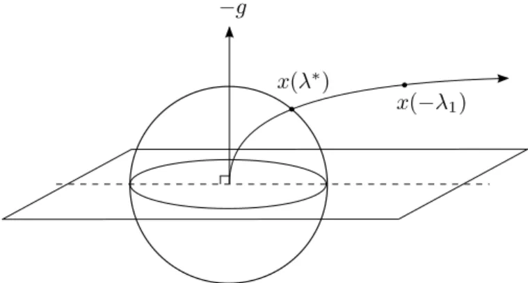
2.2.3
Case 3
In the third case, we assume that H is not positive definite, g ⊥ S1, and g 6= 0. This
situation is known as a “potential hard case.” We observe that the first term in the
eigenvector expansion (2.9) is 0, so
x(λ) =−
k
X
j=2
1 (λj +λ)
ξj(ξjTg)
!
A consequence of this formula is that the curve x(λ) is orthogonal to the eigenspace
S1. In this case, rather than going to infinity, the solution obeys
lim
λ→−λ+1
x(λ) =x(−λ1) = −
k
X
j=2
1 (λj−λ1)
ξj(ξjTg)
!
We also observe that the matrix H − λ1I is positive semidefinite. To perform the
analysis, we divide Case 3 into the following three subcases.
In the first subcase, x(−λ1) = ∆. In this unlikely situation, x(−λ1) is the solution
to (2.1), since the sufficient conditions of Lemma 2.1.2 apply. In the second subcase,
x(−λ1)>∆. As in Case 2, Lemma 2.2.5 applies. The solution to (2.1) is x∗ =x(λ∗),
Figure 2.2: Case 3, second subcase
second subcase can be seen in Figure 2.2.
In the third subcase, x(−λ1) < ∆, that is, the parameter λ reaches −λ1 before
x(λ) escapes the feasible region. The matrix H +λI is indefinite at the boundary of
the feasible region; hence, a solution in the form of x(λ) = −(H +λI)−1g does not
exist. This situation is known as the “hard case,” because we are unable to find a
solution simply by tracing the curve x(λ) to the boundary. However, after choosing
any eigenvectorξ in the eigenspaceS1, we can construct a solution to (2.1) by applying
the following lemma.
Lemma 2.2.6 For any τˆ ∈ R and ξ ∈ S1 such that kx(−λ1) + ˆτ ξk = ∆, a global
solution to (2.1) is given by x∗ =x(−λ1) + ˆτ ξ.
Proof: We have already established that the matrix H−λ1I is positive semidefinite.
Next, we consider the KKT conditions that must be satisfied by a local solution x∗.
First, we multiply the matrixH−λ1I byx(−λ1), which is the first component of the
Figure 2.3: Case 3, third subcase (the hard case)
proposed solution x∗.
(H−λ1I)x(−λ1) = −
k
X
j=2
λj
λj−λ1
(ξjTg)ξj + k
X
j=2
λ1
λj−λ1
(ξjTg)ξj
=−
k
X
j=2
(ξjTg)ξj
=−g 6= 0
The last equation holds because we have assumed that g ⊥ S1. Next, we consider the
effect of multiplying the matrix H−λ1I by ξ, as follows:
(H−λ1I)ξ= (λ1−λ1)ξ = 0
Thus (H−λ1I)(x(−λ1) +τ ξ) =−g for τ ∈R. Finally, there exist two or more values
of ˆτ >0 such that kx(−λ1) + ˆτ ξk= ∆. Thus, x∗ =x(−λ1) + ˆτ ξ satisfies the conditions
of Lemma 2.1.1, making it a global solution to (2.1).
2.2.4
Case 4
In the fourth and final case, we assume that H is not positive definite and g = 0. In
this case, x(λ) = 0 for all values of λ. We choose any eigenvector ξ of the eigenvalue
λ1, and we define
ˆ
τ = ∆
kξk.
Thenx∗ = ˆτ ξ is a solution sinceH−λ1Iis positive semidefinite, (H−λ1I)x∗ = 0 =−g,
andkx∗k= ∆. Consequently, wheng = 0, the problem (2.1) is just a problem of finding
the minimum eigenvalue of H. This relation between solving (2.1) and eigenvalue
problems will appear again in Chapters 3 and 4.
Analysis of the preceding four cases demonstrates that we can always obtain a global
solution to (2.1), even in the hard case.
2.3
Necessary and Sufficient Conditions for the
Inequality-constrained Subproblem
When linear inequality constraints are present, the KKT conditions for the
inequality-constrained trust-region subproblem (1.10) are as follows:
(H+λ∗I)x∗+g−ATω∗−λ∗x∗ = 0 λ∗(x∗Tx∗ −∆2) = 0
ω∗(Ax∗−b) = 0
kx∗k2 ≤∆2
Ax∗−b ≤0
λ∗ ≥0
ω∗ ≥0
The proposed algorithm attempts to minimize the sum of the residual norms for
the first three conditions while maintaining strict feasibility, complementary slackness,
Chapter 3
Algorithms for Trust-region
Subproblems
Having investigated the structure of the unconstrained trust-region subproblem
(2.1), we now present algorithms for approximating its solution. We begin with an
algorithm applicable to the relatively small-scale case, then proceed to review
algo-rithms for large-scale problems.
3.1
Small-scale Case
3.1.1
Positive Definite
H
Most of the early work in solving trust-region subproblems emphasized the case in
which the matrix H is positive definite. Because the underlying general nonlinear
problems were small, accuracy was not as important as it was for large-scale problems.
The “dogleg,” “double dogleg,” and “hook” methods approximate the intersection of
the parameterized solution curvex(λ) with the trust region boundary by constructing
piecewise linear approximations of x(λ) based on the Newton step xN = −H−1g. See
In the large-scale case, the factorization necessary to find a Newton step is
ineffi-cient, and it is necessary to solve trust-region subproblems more accurately to avoid an
excessive number of iterations in solving the underlying NLP. Moreover, it is generally
not easy to determine whether the matrix H is positive definite or indefinite.
In this thesis, we investigate algorithms that can solve the indefinite problem. While
our ultimate goal is to solve large-scale problems with inequality constraints, solving a
small-scale indefinite problem without inequality constraints is important in our work.
As a result, we devote some detail to explaining the method introduced by Mor´e and
Sorensen.
3.1.2
Indefinite
H
When the matrix H is indefinite and small enough to allow factorization, we can solve
(2.1) by using a method introduced by Mor´e and Sorensen [30]. In this section, we
again definex(λ) as
x(λ) =−(H+λI)−1g
for λ > −λ1, where λ1 is the minimum eigenvalue of H. We recall that when H is
indefinite, a solution to (2.1) must lie on the boundary of the sphere, with H +λI
positive semidefinite.
Rather than solve the equation
kx(λ)k= ∆ (3.1)
Mor´e and Sorensen’s method first attempts to find an approximate solution to the
equation
Φ(λ)≡ 1
∆−
1
by using Newton’s method. This choice of equation to solve makes use of the fact that
kx(λ)k2 can be rewritten as a rational function. To see this, we decompose the real
symmetric matrixH as follows:
H =BΛBT with Λ = diag(λ1, λ2, . . . , λn) andBTB =I.
Then, recalling the derivation in (2.9), we see that
kx(λ)k2 =kB(Λ +λI)−1BTgk2 =
n
X
j=1
γ2
j
(λj+λ)2
(3.3)
whereγi is theith component ofBTg. Becausekx(λ)k2 has this structure, the function
Φ(λ) defined in (3.2) is nearly linear. This allows the the solution of (3.2) to be more
easily obtained by Newton’s method than the solution to (3.1).
Having investigated the structure of kx(λ)k, we next analyze the behavior of the
function Φ(λ). The following lemma states the properties of Φ(λ) that are essential in
Mor´e and Sorensen’s algorithm.
Lemma 3.1.1 The function Φ(λ) is convex and strictly decreasing for
λ∈(−λ1,∞).
This lemma can be proved by using equations (2.5) – (2.8) and the Cauchy-Schwarz
inequality to show Φ00(λ)>0.
Starting with λ ≥ 0 (H +λI positive definite), the most basic form of Mor´e and
Sorensen’s modified Newton’s method is as follows:
1. Factor H+λI =RTR (Cholesky factorization).
2. Solve RTRx(λ) = −g.
3. Solve RTq=x(λ).
4. Update λ:
λ+ :=λ+
k
x(λ)k
kqk
2k
x(λ)k −∆
∆
(3.4)
The derivation of the updating step is as follows. Given RTRx(λ) =−g and RTq =
x(λ), we can solve forq in terms ofR and g, which yields
q =−R−T RTR−1
g
Next, using (2.8) and the fact that RTR = H +λI, we observe that we can rewrite
Φ0(λ) in terms of the norm of q:
Φ0(λ) =− kqk
2
kx(λ)k3
Finally, we can write Newton’s method for updating λ:
λ+=λ+
Φ(λ) Φ0(λ)
=λ+
1 ∆−
1
kx(λ)k kqk2
kx(λ)k3
=kx(λ)k
2
kqk2
kx(λ)k −∆
∆
The preceding expression is exactly the updating scheme from Step 4 of the basic
algorithm.
The basic algorithm suffers from three major failings; the first of these is that it
allows values of λ+ less than ˆλ = max(0, −λ1). When λ+ falls below −λ1, the matrix
H+λI is indefinite, rendering the Cholesky decomposition impossible. The algorithm
must immediately terminate without finding a solution. Even ifλ+ >−λ1, by allowing
negative values ofλ+, the algorithm becomes slower (in the best case) or misses finding
Figure 3.1: Φ(λ) withkxNk>∆, hard case not in effect
Figure 3.2: Φ(λ) withkxNk=kx(0)k<∆, hard case not in effect
The second major failing of the algorithm is that it can miss an interior solution. As
shown in Figure 3.1, ifH is positive definite and the Newton pointxN lies outside the
trust region (kxNk >∆), then the zero of the function Φ(λ) occurs for some positive
λ. In this case, the algorithm should simply locate the corresponding value ofλ. If the
Newton point is feasible, as shown in Figure 3.2, then the algorithm should terminate
with λ+ = 0 rather than find the zero of the function.
The third failing of the algorithm is that it does not include a strategy for dealing
with the hard case. In the hard case, as illustrated in Figure 3.3, the function does
Figure 3.3: Φ(λ), hard case in effect
not have a zero in the range ofλ for which H+λI is positive definite. The algorithm
should stop with λ close to −λ1 and use a strategy based on Lemma 2.2.6 to find
an approximate solution. The basic algorithm does not include any such strategy. In
particular, the algorithm breaks down wheng = 0, as the formula in Step 4 for updating
λ contains a division by zero.
To address the first two failings of the basic algorithm, Mor´e and Sorensen
incorpo-rate into their algorithm a safeguarding process. The safeguarding process updates
λ in such a way thatH+λI remains positive definite, which permits Cholesky
factor-ization. The safeguarding process also maintains an interval of decreasing length that
attempts to bracket the optimal value ofλ. The success of this process depends on the
fact that Φ(λ) is convex and strictly decreasing for values of λbetween −λ1 and ∞, as
shown in Lemma 3.1.1.
The safeguarding process requires three parameters: λL and λU, which bracket λ∗,
and λS, which is a lower bound on −λ1. λS is also used to ensure that the length of
the interval [λL, λU] decreases as the algorithm progresses. The rules used to safeguard
To address the third failing of the basic algorithm, we recall that when we are in the
hard case, we can still find a solution to (2.1). First, we must compute an eigenvector
ξ ∈ S1. Then, we can define a solution x(−λ1) +τ ξ based on Lemma 2.2.6. While
this approach is theoretically sound, determining that g ⊥ S1 and computing x(λ)
and ξ can be resource-intensive. To eliminate the need for eigenvector computations,
Mor´e and Sorensen provide a rather complicated method for approximating the desired
eigenvector. However, the methods proposed in Chapter 4 use Mor´e and Sorensen’s
algorithm to solve only very small (four- or five-dimensional) trust-region problems, so
it is efficient to approximate the eigenvectorξ by using more conventional methods.
A more complete version of Mor´e and Sorensen’s algorithm can be written as follows:
1. Safeguard λ.
2. Attempt to compute the Cholesky factorization of H+λI. If the factorization
fails, go to 5.
3. Solve RTRx=−g.
4. If kxk<∆, computeτ and ξ.
5. Update λL,λU, and λS.
6. Check the convergence criteria.
7. IfH+λI is positive definite andg 6= 0 then updateλby formula (3.4); otherwise,
λ=λS.
Mor´e and Sorensen show that the revised algorithm, when used in conjunction with
trust region methods, yields a version of Newton’s method that is robust and effective
for solving the trust-region problem.
Having explored algorithms pertinent in the small-scale case, we now turn our
at-tention to solving large-scale versions of (2.1).
3.2
Large-scale Case
In this section, we review techniques for solving (2.1) when n is very large, rendering
matrix factorization too computationally expensive to be useful. We do not assume
any knowledge about the eigenvalues of the matrixH.
3.2.1
Conjugate Gradient Methods
The conjugate gradient (CG) method, designed to solve large, sparse, symmetric
pos-itive definite linear systems, is the foundation for several methods that approximately
solve the trust-region subproblem (2.1). See Algorithm 7 in Appendix A for a
step-by-step description of the CG algorithm. WhenH is positive definite, the CG method can
be applied to the following linear system, which results from setting ∇ψ = 0:
Hx=−g (3.5)
The iterates {xk} generated by the CG method minimize the function ψ(x) over a
sequence of nested Krylov subspaces. The set {p0, p1, . . . , pk} of CG step directions is
H-conjugate (that is,pT
jHpk = 0 when j 6=k) and spans the kth Krylov subspace Kk
defined by
Kk = span
g, Hg, H2g, . . . , Hkg
In exact arithmetic, whenH is positive definite, the CG method converges to the
solu-tion of the linear system (which is the unconstrained minimum of (2.1)) inniterations.
In practical algorithms, CG iterations terminate when the norm of the residual of the
linear system falls below a specified tolerance.
If information about the matrixHis available, it is possible to improve the efficiency
matrix. Numerous preconditioners are listed with appropriate references in [25] and
[26]. Though the algorithm proposed in this thesis does not incorporate CG
precondi-tioners, it can easily be adapted to perform preconditioned CG iterations. A thorough
explanation of the CG method, including preconditioning, can be found in [25].
Steihaug-Toint
A simple modification to the conjugate gradient method proposed independently by
Steihaug [38] and Toint [40] approximately solves the trust-region subproblem (2.1).
This modification relies on the fact that when started from the origin (x0 = 0), CG
iterates increase monotonically in norm.
The Steihaug-Toint algorithm applies the CG method to the linear system (3.5),
starting at x0 = 0. At each iteration, the algorithm checks the sign of pTi Hpi, where
pi is the proposed step direction. If pTi Hpi < 0, then the matrix H is indefinite, so
the solution to (2.1) must be on the trust-region boundary. The step pi is a descent
direction for ψ(x) = 12xTHx+gTx, so the algorithm follows this step to the boundary of the trust region. It returns the boundary point as the approximate solution and
terminates. IfpT
i Hpi >0, the algorithm computes a CG step. If the proposed iterate
xi+1 would leave the trust region, the method takes the CG step in the direction ofxi+1
and stops at the boundary. The method returns this boundary point as the approximate
solution. If the proposed iterate stays within the trust region, the method takes the
full CG step and iterates again. If the CG iteration solves the linear system to within a
user-specified tolerance, the algorithm concludes that the unconstrained minimum (the
Newton pointxN) is feasible with respect to the trust-region constraint. The algorithm
returns the final iterate as an approximation ofxN.
The Steihaug-Toint algorithm has some desirable features, but it is not ideal for all
cases. The approximate solution is coarse but relatively inexpensive to compute. This
fact suggests that the algorithm can be incorporated into a trust-region framework.
Unfortunately, the algorithm does not provide any means to improve the accuracy of
boundary solutions. (The accuracy of interior solutions can be improved by decreasing
the tolerance for terminating the CG iterations, but it should be noted that CG iterates
gradually loseH-conjugacy in inexact arithmetic.) The Steihaug-Toint algorithm does
not provide any estimate of the multiplier λ∗ for the trust-region constraint, but it is
not difficult to compute an approximation. If the approximate solution is strictly inside
the trust region, then λ∗ = 0; otherwise, the least-squares approximation
λlsq =−
˜
xT(Hx˜+g)
˜
xTx˜
can be used, where ˜xis the Steihaug-Toint approximate solution. The accuracy of this
multiplier value depends, of course, on the accuracy of ˜x.
3.2.2
Lanczos Methods
The Lanczos method generates bases for the same Krylov subspacesKkas the conjugate
gradient method and provides an alternative method for solving Hx =−g when H is
positive definite. See Algorithm 8 in Appendix A.2. Instead of being H-conjugate,
the set of Lanczos vectors {q0, q1, . . . , qk} is orthonormal (in exact arithmetic). The
Lanczos vectors satisfy the following equations:
QTkHQk =Tk
QTkg =γ0e1
g =γ0q0
(3.6)
where Qk = [q0q1. . . qk], Tk is a symmetric tridiagonal matrix, γ0 = kgk, e1 is the
generated iteratively through three-term recursion relations. They are closely related
to CG residuals; in fact, they are scalar multiples of the CG residuals, and the entries
of the matrixTk can also be written in terms of the scalarsαk and βk generated in the
CG algorithm (see Appendix A.2). The CG and Lanczos iterations break down under
different conditions: the CG iteration only fails if it encounters a direction of negative
curvature (αk<0), but the Lanczos iteration breaks down if it encounters an invariant
subspaceKk. The entries of Tk remain the same from one iteration to the next except
for the addition of a new diagonal entry and a new off-diagonal entry.
In practical implementations of the Lanczos algorithm, the vectors {qk} gradually
lose orthogonality because the computations are not performed in exact arithmetic.
(CG iterates suffer a similar loss of H-conjugacy, as we mentioned in the preceding
section.) Sorensen [36] proposes an “implicitly restarted” Lanczos method that
period-ically restores the orthogonality of the vectors at a significant additional computational
cost.
Several methods for solving trust-region subproblems are powered by the
Lanc-zos method or an implicitly restarted variant. Two of these, the well-known GLTR
algorithm and the LSTRS algorithm, are introduced for the purposes of theoretical
comparison with our proposed algorithm. We also incorporate the GLTR algorithm
into our numerical tests for practical comparison. Our experience with the LSTRS
method suggests that it is not as effective as the GLTR method. For this reason we
do not include the LSTRS method in our numerical tests, despite the fact that
Kears-ley’s method (which we will discuss in Chapter 4) suggests the LSTRS method as a
subproblem solver.
GLTR
The generalized Lanczos trust region (GLTR) method of Gould, Lucidi, Toint, and
Roma [19] attempts to improve on the Steihaug-Toint strategy for solving the
trust-region subproblem (2.1). The GLTR method combines the Lanczos algorithm with
a variant of the Mor´e and Sorensen method described in Section 3.1.2. The authors
observe that for a Lanczos basis matrix Qk= [q0q1 . . . , qk], solving the problem in the
range space ofQk, that is,
minimizex∈Rn|x=Q kh
1 2x
THx+gTx
subject to: kxk2 ≤∆
is equivalent to solving the problem
minimizeh∈Rk+1 1 2h
T
Tkh+γ0eT1h
subject to: khk2 ≤∆
(3.7)
where the matrix Tk, the scalar γ0, and the vector e1 are the same as in the
Lanc-zos equations (3.6). Because the matrix Tk is tridiagonal, the computational cost of
factoring Tk is significantly smaller than the cost of factoring H. This fact makes it
feasible to solve the tridiagonal minimization problem (3.7) nearly exactly by using the
Mor´e-Sorensen algorithm. The authors make an alteration to the algorithm so that
the starting value of λ lies in the interval [max(0, θk), λk], where θk is the smallest
eigenvalue of Tk and λk is the multiplier for the solution hk of (3.7).
Algorithm 1 shows a step-by-step walkthrough of the GLTR algorithm. For more
information about the algorithm used to solve the tridiagonal trust-region subproblem,
Algorithm 1GLTR algorithm
Require: H, g, ∆
1: Initialize: x0 = 0, r0 =g, γ0 =kg0k, p0 =−g, β−1 = 0
2: Initialize: INTERIOR = true
3: for k = 0,1, . . . , until convergencedo
4: αk =rTkrk/pTkHpk
5: Update Tk−1 (usingαk and βk−1) to produce Tk
6: if INTERIOR = true, butαk ≤0 or kxk+αkpkk ≥∆ then
7: Set INTERIOR = false
8: end if
9: if INTERIOR = truethen
10: xk+1 =xk+αkHpk
11: else
12: Solve tridiagonal subproblem (3.7) to obtainhk
13: end if
14: rk+1 =rk+αkHpk
15: if INTERIOR = truethen
16: Test convergence usingkrk+1k
17: else
18: γk+1 =krk+1k
19: Test convergence usingγk+1|eTk+1hk|
20: end if
21: βk =rkT+1rk+1/rTkrk
22: pk+1 =−rk+1+βkpk
23: end for
24: If INTERIOR = false, computexk =Qkhk
Starting from the center of the trust region, the algorithm performs CG steps and
builds the matrix Tk by using the CG scalars αk and βk−1. After each CG iteration,
the algorithm checks to see whether it has encountered either a direction of negative
curvature or the boundary of the trust region. If the algorithm has encountered neither,
it continues to the next iteration. Otherwise, it concludes that the solution must be on
the boundary, so it applies the variant of the Mor´e-Sorensen algorithm to the tridiagonal
trust-region subproblem (3.7) to compute an approximate solution hk. Convergence is
indicated when the norm of the current CG residual is smaller than a user-specified
tolerance (the solution is interior) or the quantity k∇L(xk, λk)k =k(H+λkI)xk+gk
is smaller than a user-specified tolerance. The authors prove that
k(H+λkI)xk+gk=γk+1|eTk+1hk|
where γk+1 is the norm of the CG residual rk+1. This equivalence makes it possible
to measure the norm of ∇L(x, λ) without performing the change of variables xk =
Qkhk, which would cost an additional matrix-vector multiplication at each iteration and
require storage of Qk. If k∇L(xk, λk)k is not small enough, the algorithm computes
another Lanczos vector qk+1 and re-solves the tridiagonal system for another vector
hk+1. When the algorithm terminates, the multiplier λk for the solution hk of the
tridiagonal system is returned as an approximate multiplier for the original problem in
the full n-dimensional space (2.1).
The GLTR algorithm provides some improvement over the Steihaug-Toint strategy
and provides an approximate multiplier λk, but the algorithm does suffer from a few
drawbacks. When the solution of then-dimensional problem (2.1) is on the trust-region
boundary, the matrixQk must be available to make the change of variables xk=Qkhk.
for very largen) or regenerated using a set of recurrences (which requires more
matrix-vector multiplications). The GLTR algorithm is anunrestarted algorithm, which means
that the Lanczos vectors are not reorthogonalized at any point. Therefore, after many
iterations, the Lanczos matrix Qk is not orthonormal, which can compromise the
ap-proximate solution xk. The authors recommend running the algorithm no more than
five to ten iterations past the Steihaug-Toint point. If the resulting xk does not have
a significantly lower objective value than the Steihaug-Toint point, they recommend
discarding the additional computation and returning the Steihaug-Toint solution. This
saves the added computational requirement of recomputing the matrix Qk.
LSTRS
WhenH is a large, indefinite, sparse matrix, we can apply the Large-Scale Trust-Region
Subproblem (LSTRS) method of Rojas, Santos, and Sorensen [34] to find a solution to
(2.1). By adding a new parameter, this method converts the original problem into a
scalar problem that is appropriate for the large-scale case.
The method of Rojas, Santos, and Sorensen changes the original problem into an
eigenvalue problem involving a parameterized, bordered matrix. They define the
bor-dered matrix
Bα =
α gT
g H
.
and note that
α
2 +ψ(x) =
1 2(1, x
T)B α
1
x
.
Thus, for any value of our new parameter α, we can write (2.1) as
minimize 1 2y
TB αy
subject to: yTy≤1 + ∆2
eT1y= 1
(3.8)
where e1 is the first canonical unit vector in Rn+1. Finding a solution to (3.8) is
equivalent to computing a special eigenpair ofBα. First, assume that{−λ,(1, xT)T}is
an eigenpair ofBα. Then it is the case that
α gT
g H
1
x
=−
1
x
λ.
Equivalently, we have
α+λ=−gTx (3.9)
and
(H+λI)x=−g. (3.10)
Using the decomposition in (2.9), we can define the function Θ(λ) forλ≥0 as follows:
Θ(λ) =−gTx=
n
X
j=1
β2
j
λj+λ
(3.11)
Differentiating with respect toλ and recalling the definition of x(λ), we obtain
Θ0(λ) = xTx. (3.12)
smallest eigenvalue of Bα. Thus the matrix H +λ1(α)I is positive semidefinite for
all values of α. If the value of α is updated until the associated x value satisfies
Θ(λ) = α+λand Θ0(λ) = ∆2, then the first order sufficient conditions (H+λI)x=−g
andλ(∆− kxk) = 0 are satisfied with the matrixH+λI positive semidefinite. Ifλ ≥0, then the solution x lies on the boundary. If we encounter λ < 0 with kxk < ∆, then the Newton point is feasible.
The analysis just described assumes that at least one of the eigenvectors
corre-sponding to the smallest eigenvalue of Bα has a nonzero first component that can be
normalized to have the value one. Rojas, Santos, and Sorensen show that in a potential
hard case (described in Case 3 in the section “Problem Structure”), for all values of
α greater than a “critical value” ˜α1, the eigenvectors of the smallest eigenvalue of Bα
all have first component 0. This result does not invalidate the algorithm in a
poten-tial hard case; it merely requires that an alternative eigenvector be used. The authors
show that given any value of α, it is possible to find an eigenvector of Bα whose first
component can be normalized to 1. If the potential hard case is not in effect, or if the
potential hard case is in effect andα≤α˜1, then an eigenvector associated withλ1(α) is
used. If the potential hard case is in effect andαis slightly larger than the critical value
˜
α1, then an eigenvector corresponding to the second smallest eigenvalue ofBα is used.
Since an implicitly restarted Lanczos method can compute the two smallest eigenvalues
along with corresponding eigenvectors at relatively low cost (compared to the cost of
computing only the smallest eigenpair), the overall algorithm always computes both
eigenvalues and eigenvectors whenever a new eigenvector is needed.
Rojas, Santos, and Sorensen’s method usesλ, Θ(λ), and Θ0(λ) to adjust the
param-eter α by means of rational interpolation. After finding an interpolant ˆΘ, the method
locates a point ˆλ for which ˆΘ0(ˆλ) = ∆2. Then they update the parameter α via the
following equation:
α+= ˆλ+ ˆΘ(ˆλ).
As a part of the overall algorithm, the value of α+ is safeguarded, which guarantees
that the algorithm will converge. The authors prove that their algorithm is globally
convergent at a superlinear rate.
The LSTRS method offers advantages that made it Kearsley’s choice of subproblem
solver, but it has some drawbacks that caused difficulty in our numerical tests. The
algorithm is “matrix-free,” provides an approximate Lagrange multiplier for the trust
region, can handle indefinite H, and does not require modification in the hard case.
However, the method uses a large number of matrix-vector products for eigenvector
computations and can occasionally miss interior solutions in favor of boundary
solu-tions. In fact, our numerical experiments indicate that the default parameters for the
LSTRS algorithm emphasize boundary solutions.
SSM
The sequential subspace minimization (SSM) technique, which was proposed by Hager
[21] and analyzed by Hager and Park [22], iteratively projects a trust-region problem
into a smaller subspace and solves the reduced problem with an appropriate small-scale
algorithm (such as Mor´e and Sorensen’s algorithm). After changing variables back to
the full space, the solution to the reduced problem is considered an approximate solution
to the full problem. Unlike the GLTR method, which optimizes over a sequence of
nested subspaces, the SSM method optimizes over a sequence of subspaces of fixed, low
dimension. The SSM method is designed to solve the subproblem when the solution is
To generate an approximate solutionxk+1, the SSM method solves the problem
minimizex∈Sk 1 2x
THx+gTx
subject to: kxk2 = ∆
(3.13)
whereSkis the subspace spanned by a small number of vectors (four or five, in practice). A single iteration of the SSM method is presented in Algorithm 2. The columns of the
matrix Wk span the subspace Sk; Wk is updated after every SSM iteration. In this
Algorithm 2SSM Iteration
1: Determine (z∗, η∗) as the minimum eigenpair of (WkTHWk)z =η(WkTWk)z.
2: Determine (u∗, ξ∗) by solving the following minimization problem:
minimize uT(WT
kg) +
1 2u
T(WT
kHWk)u
subject to kWkuk2 ≤∆
3: Set vk+1 =Wkz∗ and λk+1 =η∗
4: Set xk+1 =Wku∗ and σk+1 =ξ∗
algorithm, (vk+1, λk+1) is an approximate minimum eigenpair ofH. The vector xk+1 is
an approximate solution to (3.13) andσk+1is the corresponding approximate multiplier.
The columns ofW include the previous iteratexk, which guarantees monotonic decrease
of the objective function; the gradient Hxk+g of the objective function at xk, which
guarantees descent if the previous iterate xk did not satisfy the KKT conditions; and
an approximate eigenvector ξ1 corresponding to the minimum eigenvalue of H, which
promotes convergence. This choice of vectors is motivated by the following theorem.
Theorem 3.2.1 (Hager and Park [22]) If in each step of SSMSk contains the
vec-tors xk, Hxk+g, and ξ1, an eigenvector associated with the smallest eigenvalue λ1 of
H, then SSM converges to a solution of (3.13).
Note that in practice the exact minimum eigenpair is not known, so convergence is not
guaranteed.