WATER BALANCE CHANGE UNDER CLIMATE AND LANDUSE/LANDCOVER VARIABILITY IN
THE NORTH CAROLINA PIEDMONT
Yuri Kim
A dissertation submitted to the faculty of the University of North Carolina at Chapel Hill in
partial fulfillment of the requirements for the degree of Doctor of Philosophy in the
Department of Geography
Chapel Hill
2012
Approved by:
Lawrence E. Band
Aaron Moody
Chip Konrad
Conghe Song
iii
Abstract
YURI KIM: WATER BALANCE CHANGE UNDER CLIMATE AND LANDUSE/LANDCOVER VARIABILITY IN THE NORTH CAROLINA PIEDMONT
(Under the direction of Lawrence E. Band)
Fresh water availability is an important concern for human society as well as ecosystems. In this dissertation, water resources trends in the North Carolina Piedmont were analyzed to
understand historical trends and provide potential future scenarios in response to different climate and landuse/landcover (LULC) dynamics. North Carolina Piedmont has experienced a large scale LULC conversion from farmland to naturally grown forest, followed by recent urbanization, in the last century. Simulation with the Soil and Water Assessment Tool (SWAT) indicates that forest re-growth mitigated the impact of increased precipitation on stream discharge in areas that reforested from abandoned agricultural fields due to increasing water consumption. For projected climate conditions, nested global and regional circulation model results from the North American Regional Climate Change Assessment Program (NARCCAP) were evaluated for bias relative to current measurements in North Carolina. For historical NARCCAP output (1971-2000), precipitation shows seasonal bias pattern and, there is a general trend of NARCCAP temperature cold bias. After
iv
evapotranspiration (ET) is projected to increase in winter and spring while annual water yield (WY) would show various changing patterns, with greater dependence on projected CO2 and
v
This dissertation is dedicated
vi
ACKNOWLEDGEMENTS
First, I would like to show my very special thanks to my advisor, Dr. Lawrence Band who support me by deepening and broadening my research views. I am so lucky to meet such an
enthusiastic and erudite advisor as I also get his energy when I am with him. He is my role model not only for an academic advisor but also as a lifetime mentor.
I am also grateful to other committee members, Dr. Aaron Moody, Dr. Chip Konrad, Dr. Conghe Song, and Dr. Philip Berke. I learned a lot not only from their classes but also in personal conversation and discussion over the years. They also showed interests to my researches and gave me chance to “think outside the box” way by guiding me with different perspectives that I have never considered. In addition, I also like to thank my colleagues (Band group people) and friends who helped me for the completion of this dissertation; special thanks to Brian Miles who gave me valuable feedbacks to improve my dissertation both academically and grammatically.
vii
TABLE OF CONTENTS
LIST OF TABLES ... xi
LIST OF FIGURES ... xii
Chapter 1: Introduction ... 1
References ... 6
Chapter 2: The influence of forest re-growth on the stream discharge in the North Carolina Piedmont watersheds... 7
2.1 Abstract ... 7
2.2 Introduction ... 8
2.3 Methodology ... 12
2.3.1 Study areas ... 12
2.3.2 LULC change history ... 15
2.4 Simulation with SWAT and Weather Data ... 20
2.5 Results ... 23
2.5.1 Precipitation and Stream Discharge trends ... 23
2.5.2 SWAT Calibration and validation ... 26
2.5.3 Water year scale SWAT simulation since 1920 ... 31
viii
2.5.5 SWAT simulation with 1955 LULC... 38
2.5.6 SWAT simulation differences between 1955 and 2006 LULC ... 40
2.6 Discussion ... 43
2.7 Conclusion ... 46
References ... 47
Chapter 3: Evaluation and bias correction of NARCCAP nested General Circulation Models (GCMs) and Regional Climate Models (RCMs) precipitation and temperature in North Carolina for hydrologic model application ... 49
3.1 Abstract ... 49
3.2 Introduction ... 50
3.3 Methods ... 55
3.3.1 Evaluation of North American Regional Climate Change Assessment Program (NARCCAP) GCM-RCM precipitation and temperature ... 55
3.3.2 Bias correction of NARCCAP GCM-RCM precipitation and temperature ... 59
3.3.3 Raw and bias-corrected NARCCAP GCM-RCM precipitation and temperature application to SWAT modeling ... 63
3.4 Results ... 66
3.4.1 Evaluating NARCCAP output ... 66
3.4.2 NARCCAP bias correction: Calibration and Validation ... 69
3.4.3 NARCCAP application to a hydrologic modeling ... 81
3.5 Discussion ... 83
ix
References ... 88
Chapter 4: Simulation of future water yield under the condition of changing CO2, climate and landuse/landcover (LULC) in the North Carolina Piedmont ... 90
4.1 Abstract ... 90
4.2 Introduction ... 91
4.3 Study area ... 94
4.4 Method ... 100
4.4.1 Climate model output: North American Regional Climate Change Assessment Program (NARCCAP) ... 100
4.4.2 LULC map for SWAT application ... 101
4.4.3 Hydrologic model simulation (SWAT) with both measured and climate model output in historical time period ... 102
4.4.4 Hydrologic model simulation with projected CO2 concentration and climate ... 103
4.4.5 Hydrologic model simulation with projected LULC ... 104
4.4.6 Hydrologic model simulation with projected CO2, climate and LULC ... 105
4.5 Results ... 105
4.5.1 NARCCAP bias correction in historical data ... 105
4.5.2 Hydrologic simulation with historical time ... 109
4.5.3 Hydrologic simulation with future changing environment ... 113
4.6 Discussion ... 129
4.6.1 Uncertainty in interaction between CO2 increasing, forest ET and growth ... 129
x
4.6.3 SWAT simulated ET difference between coniferous and deciduous forest under
projected CO2 and climate ... 136
4.6.4 SWAT simulated WY change in watersheds with ICLUS SERGoM A2 urban growth scenario in 2060 ... 139
4.6.4 Inter-annual variability of ET and WY in projected changing environment ... 142
4.7 Conclusion ... 146
References.. ... 147
Chapter 5: Summary and Conclusions... 151
xi
LIST OF TABLES
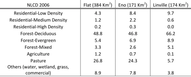
Table 2.1: Current percent LULC condition of three study watersheds by NLCD 2006
(http://www.mrlc.gov/nlcd06_data.php) ... 14 Table 2.2: Major LULC changes from 1955 to 2006 in the Flat River watershed ... 19 Table 2.3: Daily scale calibration and validation results of three study watersheds by Nash-Sutcliff Efficiency (NSE) of stream discharge (Q). Calibration and validation period are two years each ... 27 Table 2.4: Monthly scale SWAT simulation best result of three study watersheds by Nash-Sutcliff Efficiency (NSE) of stream discharge (Q) from 1986 to 2009. ... 33 Table 3.5: Daily maximum temperature (Tmax) second order Fourier transformation results, R2 ... 74 Table 3.6: Daily minimum temperature (Tmin) third order Fourier transformation results, R2 ... 74 Table 4.1: Landuse/Landcover (LULC) of three study watersheds in current time by NLCD 2006 (%) 98 Table 4.2: LULC change by EPA ICLUS SERGoM A2 scenario ( %) ... 99 Table 4.3: Future water availability by projected CO2 and climate scenarios. “Measured” data is
observed data in 1974-2000 “Historical NARCCAP” is climate model output in 1974-2000, and “Future NARCCAP” is climate model output in 2044-2070 ... 114 Table 4.4: Future water availability by projected CO2, climate, and LULC scenarios. “Measured”
climate data is observed data in 1974-2000, “Current” LULC is NLCD 2006 + ICLUS 2010 A2 composite map, “Future NARCCAP” is climate model output in 2041-2070, and “Future (2060)” LULC is for ICLUS 2060 A2 LULC. ... 121 Table 4.5: Three month averaged monthly scale WY change in low flow (CDF 0.1 level) under
xii
LIST OF FIGURES
Figure 2.1: Historical Palmer Drought Severity Index (PDSI) and Palmer Hydrological Drought Index (PHDI) in North Carolina by water year scale. Climate Division 3 is the Northern
Piedmont, and Climate Division 1 is the Southern Mountain (NOAA Satellite and
Information Service, http://www.ncdc.noaa.gov) ... 10
Figure 2.2: The geographic division of North Carolina: Mountain (left), Piedmont (middle), and Coastal plain (right). (a) is the long-term forested Linville River watershed, and (b) shows the reforested the Flat and the Eno River watersheds. The Flat and the Eno River
watersheds are headwater area of Falls Lake. ... 14
Figure 2.3: An example of the agricultural statistics of the North Carolina Piedmont, Person County. (a) Farm land change from 1900 to 2007 (All land in farms = total crop land + total pasture land + total woodland + all other land in farm), and (b) total crop land and harvested crop land change from 1925 to 2007(Total Crop land = harvested crop land + failed crop land + idle + plowable pasture land) (USDA Agricultural census,
http://www.agcensus.usda.gov/Publications/Historical_Publications/index.php). ... 16
Figure 2.4: Person County landuse/landcover (LULC) change in 1955 (by aerial photo) and current (by NLCD 2006) ... 18 Figure 2.5: Flat River watershed classified LULC: (a) 1955 air photo classification and (b) NLCD 2006
... 18
Figure 2.6: Examples precipitation and stream discharge trends of LULC conversion from agricultural to forest area (the Flat and the Eno River watersheds in North Carolina Piedmont) and long term consistent forest area (the Linville River watershed ) in North Carolina
Mountain (http://waterdata.usgs.gov/nwis; http://climod.srcc.lsu.edu/) ... 25 Figure 2.7: Flat River watershed calibration (left) and validation (right) result in arithmetic scale
(upper) and logarithmic scale (lower) in daily scale. The 95% confidence boundary in simulations results is drawn from simulations with a threshold of 0.5 for both NSE of stream and logarithmic scale stream discharge. ... 28 Figure 2.8: Eno River watershed calibration (left) and validation (right) result in arithmetic scale
xiii
Figure 2.9: Linville River watershed calibration (left) and validation (right) result in arithmetic scale (upper) and logarithmic scale (lower) in daily scale. The 95% confidence boundary in simulations results is drawn from simulations with a threshold of 0.5 for both NSE of stream and logarithmic scale stream discharge. ... 30 Figure 2.10: Long-term SWAT scenario simulations of the Flat and the Eno river watershed (LULC
conversion watersheds), and Linville river watershed (long-term forested watershed) in water year scale. The 95% confidence boundary in simulations results is drawn from simulations with a threshold of 0.5 for both NSE of stream and logarithmic scale stream discharge. ... 34 Figure 2.11: Flat River watershed monthly scale stream discharge residual (USGS – SWAT,
mm/month) patterns in month by month from 1926 to 2009 (*** p < 0.001, ** p < 0.01, * p < 0.05). ... 36
Figure 2.12: Linville River watershed monthly scale stream discharge residual (USGS – SWAT, mm/month) patterns in month by month from 1926 to 2009 (*** p < 0.001, ** p < 0.01, * p < 0.05). ... 37 Figure 2.13: The Flat River watershed SWAT simulation using 1955 LULC as a landuse input in water
year scale. The 95% confidence boundary in simulations results is drawn from simulations with a threshold of 0.5 for both NSE of stream and logarithmic scale stream discharge. . 39
Figure 2.14: The Flat River watershed SWAT simulated hydrologic components with 2006 and 1995 LULC. Total Water Yield (WY) from Hydrologic Response Unit (HRU) to stream channel = Surface runoff + Groundwater flow from shallow aquifer + Lateral Flow from soil profile – transmission loss from stream bed – reservoir extraction. Transmission loss and reservoir extraction are not considered because these are negligible amount. ... 42 Figure 2.15: Three month average monthly SWAT simulated stream discharge cumulative
distribution function in the Flat River watershed in 1926 – 2009 ... 45 Figure 3.1: An example of NARCCP regional climate model boundary, Regional Climate Model
version 3 (RCM3), in North Carolina ... 58
Figure 3.2: Monthly scale observed regional precipitation, maximum and minimum temperature statistics in North Carolina for two 15 year periods: 1971-1985 and 1986-2000 ... 60
Figure 3.3: Raw NARCCAP monthly scale averaged (a) precipitation, (b) maximum, and (c) minimum daily temperature for 1971~1999 in the Mountain, Piedmont, and Coast of North
xiv
Figure 3.4: Five NARCCAP precipitation monthly scale “wet day threshold” for 1) two time periods for calibration and validation, 1971~1985 (upper) and 1986~2000 (lower), and 2)
geographical region ... 70
Figure 3.5: Five NARCCAP precipitation monthly scale “scaling factor” for 1) two time periods for calibration and validation, 1971~1985 (upper) and 1986~2000 (lower), and 2)
geographical regions ... 70 Figure 3.6: Seasonal precipitation CDF of monthly scale averaged precipitation bias correction by
1985 calibration (Corrected 1) and 1986-2000 calibration (Corrected 2) in 1971-1999 ... 72 Figure 3.7: Daily scale residual fitting by Fourier second order in Tmax (left) and Fourier third order
Tmin (right) Fourier transformation curve fitting (1986 – 2000 averaged value) ... 75 Figure 3.8: Seasonal precipitation CDF of monthly scale averaged Tmax bias correction by 1971-1985 calibration (Corrected 1) and 1986-2000 calibration (Corrected 2) in 1971-1999 ... 78 Figure 3.9: Seasonal precipitation CDF of monthly scale averaged Tmin bias correction by 1971-1985 calibration (Corrected 1) and 1986-2000 calibration (Corrected 2) in 1971-1999 ... 79 Figure 3.10: Monthly by month averaged bias corrected NARCCAP by 1986-2000 calibration.
Monthly precipitation sum and monthly averaged temperatures (Tmax and Tmin) were averaged for 1971-1999 ... 80 Figure 3.11: Haw River basin SWAT calibration result in monthly scale ... 82
Figure 3.12: Haw River basin SWAT simulation with raw NARCCAP (left) and bias corrected NARCCAP (right) ... 82 Figure 4.1: Four study watersheds in the North Carolina Piedmont with NCAR Community Climate
System Model (CRCM) grid points from North American Regional Climate Change
Assessment Program (NARCCAP) ... 95
Figure 4.2: Projected LULC change by ICLUS SERGoM of two Piedmont basins (Haw and Neuse River, top) and (a) the Eno River, (b) the New Hope Creek, and (c) the Crabtree Creek
xv
Figure 4.4: Four study watersheds NARCCAP bias corrected projected precipitation and temperature in month by month average (2041 – 2070) ... 108
Figure 4.5: SWAT calibration results of four study watersheds in monthly scale ... 111 Figure 4.6: Four study watersheds SWAT simulation with NARCCAP bias uncorrected (left) and bias
corrected (right) precipitation and temperature ... 112 Figure 4.7: SWAT simulated Evapotranspiration (ET) and water yield (WY) change by increasing CO2
from 330 to 600 ppm in the Haw River basin ... 114 Figure 4.8: Monthly scale averaged (1974 – 1999) SWAT simulated Evapotranspiration (ET) change
by projected CO2 and climate change scenarios in the Haw River basin ... 116 Figure 4.9: Monthly scale averaged (1974 – 1999) SWAT simulated total Water Yield (WY) change by projected CO2 and climate change scenarios in the Haw River basin ... 118 Figure 4.10: Haw River basin water yield change by projected changing CO2 and climate scenarios in
warm and cold seasons. This box plot indicates median (central mark in box), 25th and 75th percentiles in each lower and upper edge, and extreme values with whiskers. Outliers are excluded in this plot, and average value of each scenario result is presented with dot inside the box ... 119
Figure 4.11: SWAT simulated Evapotranspiration (ET) and total Water Yield (WY) change by ICLUS SERGoM projected LULC in 2060 ... 122 Figure 4.12: Warm season (March – September) ET change by projected changing environment (CO2,
climate, and LULC) scenarios in 2061 – 2070. This box plot indicates median (central mark in box), 25th and 75th percentiles in each lower and upper edge, and extreme values with whiskers. Outliers are excluded in this plot, and average value of each scenario result is presented with dot inside the box. ... 124 Figure 4.13: Cold season (October – February) ET change by projected changing environment (CO2,
climate, and LULC) scenarios in 2061 – 2070. This box plot indicates median (central mark in box), 25th and 75th percentiles in each lower and upper edge, and extreme values with whiskers. Outliers are excluded in this plot, and average value of each scenario result is presented with dot inside the box. ... 125 Figure 4.14: Warm season (March – September) WY change by projected changing environment
xvi
with whiskers. Outliers are excluded in this plot, and average value of each scenario result is presented with dot inside the box. ... 127
Figure 4.15: Cold season (October – February) WY change by projected changing environment (CO2, climate, and LULC) scenarios in 2061 – 2070. This box plot indicates median (central mark in box), 25th and 75th percentiles in each lower and upper edge, and extreme values with whiskers. Outliers are excluded in this plot, and average value of each scenario result is presented with dot inside the box. ... 128
Figure 4.16: Monthly scale averaged (1974 – 1999) SWAT simulated Leaf Area Index (LAI) change by projected CO2 and climate change scenarios in the Haw River basin ... 133 Figure 4.17: Monthly average values of SWAT simulated stress factor (water, temperature, nitrogen,
and phosphorous) changes by projected CO2, and CCSM-CRCM temperature and
precipitation change scenarios (2044 – 2070) ... 134
Figure 4.18: Monthly average values of SWAT simulated stress factor (water, temperature, nitrogen, and phosphorous) changes by projected CO2, and NARCCAP temperature and
precipitation change scenarios (2044 – 2070) ... 135 Figure 4.19: SWAT simulated monthly scale averaged ET (2044 – 2070) of deciduous (FRSD) and
coniferous (FRSE) forest under climate and CO2 changing environments in the Haw River basin. Presented value is the average of five NARCCAP applied SWAT results. ... 137 Figure 4.20: Monthly scale deciduous and coniferous forest ET change by projected changing CO2
and climate scenarios in warm and cold seasons in the Haw River basin. Presented value is the average of five NARCCAP applied SWAT results. This box plot indicates median (central mark in box), 25th and 75th percentiles in each lower and upper edge, and extreme values with whiskers. Outliers are excluded in this plot, and average value of each scenario result is presented with dot inside the box ... 138 Figure 4.21: Three month average monthly water yield cumulative distribution function in
watersheds with projected climate, LULC, and CO2 in 10 year period (reference: 1991 – 2000 and scenario: 2061 – 2070). Presented values are the average of five NARCCAP applied SWAT results. ... 141 Figure 4.22: Haw River basin SWAT simulated water year scale WY and ET inter-annual variability for 27 years (reference: 1974 – 2000 and scenario: 2044 – 2070) ... 144 Figure 4.23: SWAT simulated water year scale WY and ET inter-annual variability for 10 years
xvii
Chapter 1: Introduction
Fresh water availability is an important concern for human society as well as ecosystems. In the Southeast of the United States, as in other locations around the globe, increases in population and demand for water along with the potential for significant change in watershed runoff
production is creating challenges and uncertainty in water security. Impacts and interactions between climate change, land use conversion and ecosystem adjustment in terms of resulting hydrologic changes are important to evaluate and de-convolve to inform water resources planning and watershed management. The main objective of this study is the integration of climate and LULC change scenarios to model and project historic and future changes in freshwater availability in the North Carolina Piedmont. Therefore, water resources trend of the North Carolina Piedmont in past and future times in response to individual and combined effects of all three of these drivers were analyzed and simulated by hydrologic model in order to understand historical trends and provide information on potential future scenarios in response to different climate and land cover dynamics.
The study area, the North Carolina Piedmont, has experienced a large scale landuse
2
Forsyth counties) regions of North Carolina Piedmont experienced unprecedented population growth rates of from 10% to 25% (2010 US Census). According to the Spatially Explicit Regional Growth Model (SERGoM) (Theobald, 2005) from the spatial allocation model of Integrated Climate and Land Use Scenarios (ICLUS) by EPA (2009), some watersheds of the North Carolina Piedmont area could have a twofold increase in urban land compared to current landcover in the future, 2060, as well. Therefore, the North Carolina Piedmont is characterized by rapid urban growth while retaining a large area of forest cover in the recent past and is expected to maintain that trend over the next few decades.
For future climate, the North American Regional Climate Change Assessment Program (NARCCAP) is selected for projected climate scenarios. NARCCAP is an international program developed to produce high resolution climate change simulations in order to investigate
uncertainties in regional scale projections of future climate and generate climate change scenarios for use in impacts research (http://www.narccap.ucar.edu). It provides a set of regional climate models (RCMs) nested within a set of atmosphere-ocean general circulation models (AOGCMs) over a domain covering the conterminous United States, most of the Canada, and Northern Mexico. The Integrated Climate and Land Use Scenarios (ICLUS) (EPA, 2009) program is used to project
LandUse/LandCover (LULC) scenarios, and is focused on urban growth. This is basically an urban expansion model using forecasted population growth and transportation infrastructure as land-use change drivers. Selected future climate CO2 concentrations and LULC scenarios are based on the same economic storyline, the Special Report on Emission Scenario (SRES) (IPCC, 2000) A2 emissions scenario for the 21st century.
The hydrologic model used to evaluate runoff impacts of LULC and climate scenario
3
et al., 2009). It is a process-based model, which requires specific information about weather, topography, soil, and LULC (i.e. vegetation, land cover and land management practices) as model input. The physical processes associated with water storage and flux, sediment transport, crop growth, nutrient cycling etc. are simulated by SWAT in a watershed. The National Elevation Dataset (NED) (http://ned.usgs.gov/) and 1:24,000 stream network data (http://www.cgia.state.nc.us/) are used for watershed and sub-watershed delineation. Each sub-watershed is divided into smaller segments, Hydrologic Response Units (HRUs), by unique LULC, soil, and management combinations. The Generalized Likelihood Uncertainty Estimation (GLUE) (Free and Binley, 1992) is applied to calibrate the model for daily runoff data under current land cover and represent uncertainty in the model predictions. GLUE is a Monte Carlo simulation-based method, developed from the
Generalized Sensitivity Analysis (GSA) of Spear and Hornberger (1980). The basic concept of GLUE is that there is no one optimal parameter set for a given watershed; a number of combinations of parameters that simulate observed discharge data can exist. The GLUE method evaluates sensitivity of each parameter and suggests acceptable parameter value combinations based on a likelihood function. The sensitivity of parameters can be explained as “behavioral” and “non-behavioral” by certain criteria for model rejection. SWAT-CUP4 software (Abbaspour, 2011), which provides for sensitivity analysis, calibration, validation, and uncertainty analysis for the SWAT model, is used for GLUE application.
The three related themes of this dissertation are:
4
2. Evaluation and bias correction of General Circulation Model (GCM) based Regional Climate Models (RCMs) precipitation and temperature in North Carolina for future water yield change scenario applications
3. Simulation of future water yield under the conditions of changing CO2, climate and landuse/landcover (LULC) in the North Carolina Piedmont
Chapter 2 focuses on the relationship between historical landuse/landcover (LULC), recent climate trends and stream discharge with the following scientific question:
How has historical forest re-growth from abandoned agricultural areas affected stream discharge of the North Carolina Piedmont catchments?
Hypothesis
H0: A hydrologic model with consistent land use explains historical behavior of watersheds that have had changing land uses.
H1: The apparent difference in runoff can be explained by land use change.
Chapter 3 is about the evaluation and bias correction of dynamically downscaled climate model information required for watershed simulation in North Carolina. The performance of a set of the nested global and regional circulation model (GCM-RCM) results from the North American Regional Climate Change Assessment Program (NARCCAP) is evaluated for bias relative to current measurement in North Carolina.
Are systematic biases found in NARCCAP produced GCM-RCM daily precipitation, and maximum and minimum temperature in the North Carolina region?
5
Is bias correction of NARCCAP necessary for its application to hydrologic modeling? To what extent can bias corrected NARCCAP output improve hydrologic modeling
performance?
Finally in Chapter 4, future water yield change sensitivity under increasing carbon dioxide (CO2), projected climate and Landuse/Landcover (LULC) variability in the North Carolina Piedmont is evaluated.
How will evapotranspiration (ET) and water yield (WY) be affected by future CO2 level and climate scenarios which generally include temperature increases and stable or moderate increases in precipitation?
6
References
Abbaspour KC, 2011. SWAT-CUP4: SWAT Calibration and Uncertainty Programs – A User Manual. Eawag: Swiss Federal Institute of Aquatic Science and technology.
Arnold J, Srinivasan R, Muttiah R, Williams J, 1998. Large area hydrologic modeling and assessment - Part 1: Model development. J.Am.Water Resour.Assoc. ;34(1):73-89.
Beven K, Binley A, 1992. The Future of Distributed Models - Model Calibration and Uncertainty Prediction. Hydrol.Process. ;6(3):279-98.
Billings WD, 1938. The structure and development of old field shortleaf pine stands and certain associated physical properties of the soil. Ecol.Monogr. ;8:437-500.
Center for Geographic Information and Analysis, 1:24,000 stream network data. http://www.cgia.state.nc.us/
Christensen N, Peet R, 1984. Convergence during Secondary Forest Succession. J.Ecol. ;72(1):25-36. Intergovermental Panel on Climate Change (IPCC), 2000. Emission Scenarios. Cambridge University Press, UK. pp 570
Multi-Resolution Land Characteristics Consortium (MRLD), National Land Cover Database 2006 (NLCD2006). http://www.mrlc.gov/nlcd06_data.php
Neitch SL, Arnold JG, Kiniry JR, Williams JR, 2011. Soil and Water Assessment Tool Theoretical Documentation Version 2009. Texas Water Resources Institute Technical Report No. 406, Texas A&M University System, College Station, Texas, USA.
North American Regional Climate Change Assessment Program (NARCCAP) project. http://www.narccap.ucar.edu
Oosting H J, 1942. An ecological analysis of the plant communities of Piedmont, North Carolina, Amer Midland Nat, 28, 1-126.
Spear R, Hornberger G, 1980. Eutrophication in Peel Inlet .2. Identification of Critical Uncertainties Via Generalized Sensitivity Analysis. Water Res. ;14(1):43-49.
Theobald, D. M.: Landscape patterns of exurban growth in the USA from 1980 to 2020, Ecol. 5 Soc., 10, 1, 32 [online] URL: http://www.ecologyandsociety.org/vol10/iss1/art32/, 2005. Unite States Environmental Protection Agency, 2009. Integrated Climate and Land-Use Scenarios (ICLUS) project. http://www.epa.gov/ncea/global/iclus/
Chapter 2: The influence of forest re-growth on the stream
discharge in the North Carolina Piedmont watersheds
2.1 Abstract
This study focuses on the relationship between historical landuse/landcover (LULC), recent climate trends and stream discharge. A major problem recognized in water resources is the issue of non-stationarity in climate and watershed conditions, and impacts on forecasting and explaining hydrologic behavior. Over the 20th century, landuse/landcover in the Southeast US, particularly the North Carolina Piedmont, has evolved from a more dominantly agricultural to an extensively forested landscape, and more recent localized urbanization. The re-growth of forests has an
important influence on the hydrology of the region as it enhances ecosystem interaction with recent climate change. During the time period of this study, 1920’s-2009, the amount of precipitation in some parts of the North Carolina Piedmont forest re-growth area showed increasing trends without corresponding increments in stream discharge. To understand the effect of LULC on runoff, we employed long-term the Soil and Water Assessment Tool (SWAT) to simulate hydrologic behavior for several watersheds in North Carolina with different LULC histories: (1) LULC conversion from
agricultural to forested area, and (2) long-term stable forest cover with no significant LULC conversion. Comparing stream discharge simulated with SWAT with the assumption of constant LULC with USGS-measured stream discharge, we found significant stream discharge
8
with long-term stable forest cover does not show this under-prediction bias; simulated and measured stream discharge show similar patterns during the entire study time period. Monthly scale residual analysis in reforested watersheds also shows significant seasonal patterns in stream discharge differences before and after forest re-growth. Therefore, the under-prediction bias of SWAT from the 1920’s to the mid-1970’s indicates that forest re-growth mitigated the impact of increased precipitation on stream discharge in the reforested area from abandoned agricultural fields due to increasing water consumption driven by changes in vegetation.
2.2 Introduction
Recent severe hydrologic droughts in the North Carolina in past decades have raised significant concerns about the adequacy of water resource systems in this area given significant population increases and potential changes in hydro-climate. In 2002 and again from 2007 to 2008, USGS stream discharge data for the Flat River in the North Carolina Piedmont (site number 0208550) documented record low flows, with zero stream discharge in October 2007 and almost zero stream discharge in summer of 2007 and 2008 (http://waterdata.usgs.gov/nc/nwis). These no-flow
conditions had not been previously experienced in 83 years of discharge records. Non-stationarity in the processes controlling watershed hydrology has been recognized as a major challenge for
evaluating and planning for water resources (Milly et al., 2008). In the Southeast United States, major shifts in land cover and climate may have produced large changes in expected runoff, as well as hydrologic extremes of floods and droughts. Therefore, planning for water security based on only past hydrologic records may not be as reliable as it appears by leading to significant bias in
9
Over the past century, a general increase in stream discharge has been found in most of the US, particularly in the eastern half (McCabe and Wolock, 2002) and is correlated with a trend of increasing precipitation (Lins and Slacks 1999, 2005; Andreadis 2006; Small et al. 2006). However, Lins and Slacks (2005) noted that stream discharge in the South Atlantic-Gulf region shows a decreasing trend especially in the annual minimum, Q0 percentile flow. This implies that either precipitation is anomalous compared to most of the US or another factor, LULC change, may affect decreasing stream discharge trend in Southeast US.
10
Figure 2.1: Historical Palmer Drought Severity Index (PDSI) and Palmer Hydrological Drought Index (PHDI) in North Carolina by water year scale. Climate Division 3 is the Northern Piedmont, and Climate Division 1 is the Southern Mountain (NOAA Satellite and Information Service,
11
Other observations suggest that LULC change may play a key role in increased drought vulnerability in North Carolina Piedmont. Figure 2.1 shows the drought indices of the Northern Piedmont (Climate Division 3) and Southern Mountain (Climate Division 1) of North Carolina. The Palmer Drought Severity Index (PDSI) is based on a water balance derived from precipitation and temperature, and Palmer Hydrological Drought Index (PHDI) is based on the hydrological impact of drought, such as reservoir and groundwater levels (NOAA Satellite and Information Service, (http://www.ncdc.noaa.gov)). Comparing these two indices in these two Climate Divisions, the lowest value of indices in Southern Mountain shows similar timing between PDSI and PHDI, whereas Northern Piedmont shows a little different timing. In the North Carolina Piedmont, the recent water shortage in 2002 recorded as the lowest hydrologic drought event in PHDI, but PDSI shows more severe meteorological droughts in 1920’s and 1930’ than 2002. Differences in timing and severity between meteorological and hydrological droughts are further evidence that factors aside from climate may be involved in drought conditions in the North Carolina Piedmont region.
We hypothesize that the severity of hydrologic drought in recent years in the North Carolina Piedmont has been influenced by LULC, i.e., forest re-growth in abandoned agricultural field during the 20th century. Reforestation can reduce annual water yield from a watershed (e.g. Hibbert 1967; Bosch and Hewlett, 1982; Trimble et al., 1987; Scott and Smith 1997; Farley et al., 2005; Huxman et al., 2005; Scott et al., 2006; Buttle, 2011). Specifically, runoff reduction by forest re-growth has a much higher impact in the dry season and in areas that have low base flow (Trimble et al., 1987; Scott and Smith 1997; Farley et al., 2005). In terms of the amount of reforestation, even a relatively small increase in forest, e.g. 10% in total area, can cause noticeable decreases in water yield (Trimble et al., 1987). Therefore, the hypothesis in this study area is that increasing water
12
Scientific question and hypothesis addressed in this study is:
How has historical forest re-growth from abandoned agricultural areas affected stream discharge of the North Carolina Piedmont catchments?
Then, two hypothesis of this question are:
H0: A hydrologic model with consistent land use explains historical behavior of watersheds that have had changing land uses.
H1: The apparent difference in runoff can be explained by land use change.
2.3 Methodology
2.3.1 Study areas
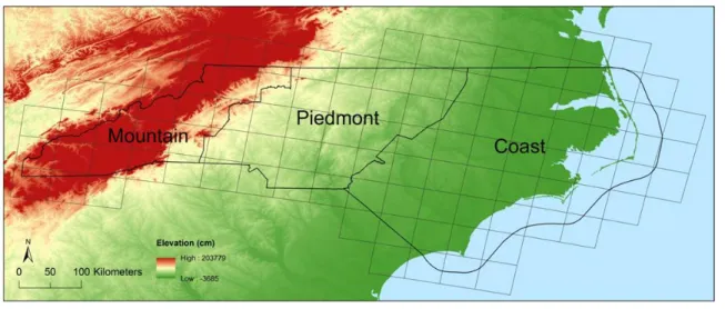
The North Carolina Piedmont has experienced a large scale landuse conversion from farmland to forest (Billings 1938; Oosting 1942; Christensen and Peet 1984). Since the region’s climate is favorable to agriculture with rolling topography with mild and humid weather, large forest areas were cleared for agricultural activity during early settlement in the eighteenth century
through the mid-nineteenth century. However, erosion and loss of the top soil reduced productivity, and cultivated patches had been gradually abandoned (Oosting, 1942). This process was hastened by food imported from the Midwest and the economic depression of the 1930’s. Current forested area of the North Carolina Piedmont mostly results from extensive secondary succession from abandoned farms.
13
watershed, located in Person County and the Eno River watershed, in Orange County, satisfy these two conditions (Figure 2.2 (b)). Additionally, these two watersheds are headwater for Durham and Raleigh water supply. Therefore, drought signals of these head water catchments can be a direct sign of water shortage for these areas. Drainage areas, length of discharge records and current land use for each watershed are given in Table 2.1.
Another study watershed with long-term forested LULC was selected to compare hydrologic behavior difference between LULC conversion and non-conversion watershed. Agriculture to forest conversion was widespread in the Piedmont of North Carolina, and there are no watersheds with long-term runoff records with consistent forest cover for comparison. However, the adjacent Blue Ridge Mountains has had consistent forest cover, although the structure of the forest has changed due to extensive past logging. The Linville river watershed which keeps a long history of
14
Figure 2.2: The geographic division of North Carolina: Mountain (left), Piedmont (middle), and Coastal plain (right). (a) is the long-term forested Linville River watershed, and (b) shows the reforested the Flat and the Eno River watersheds. The Flat and the Eno River watersheds are headwater area of Falls Lake.
Table 2.1: Current percent LULC condition of three study watersheds by NLCD 2006 (http://www.mrlc.gov/nlcd06_data.php)
NLCD 2006 Flat (384 Km2) Eno (171 Km2) Linville (174 Km2)
Residential-Low Density 4.3 8.4 9.7
Residential-Medium Density 1.2 2.2 0.6
Residential-High Density 0.2 0.3 0.0
Forest-Deciduous 48.8 46.8 66.2
Forest-Evergreen 5.4 6.9 8.9
Forest-Mixed 3.3 2.6 5.1
Agriculture 1.2 0.7 0.1
Pasture 26.8 24.3 5.7
Others (water, wetland, grass,
15 2.3.2 LULC change history
16
Figure 2.3: An example of the agricultural statistics of the North Carolina Piedmont, Person County. (a) Farm land change from 1900 to 2007 (All land in farms = total crop land + total pasture land + total woodland + all other land in farm), and (b) total crop land and harvested crop land change from 1925 to 2007(Total Crop land = harvested crop land + failed crop land + idle + plowable pasture land) (USDA Agricultural census,
17
In addition to county level agricultural census information, aerial photos in 1955 (USDA aerial photography, 1955) are used to compare land cover with current conditions. In Figure 2.4, a decrease in agricultural land use and an increase in forest cover can be detected by comparing the 1955 aerial photo with the 2006 National Land Cover data (NLCD). Numerous agricultural patches found in the 1955 aerial photos were identified as forests in the 2006 NLCD. The aerial photo of the Flat river watershed was classified with on screen digitization (Song 2012, personal communication) (Figure 2.5(a)). While care needs to be taken comparing aerial photographic interpretation with the NLCD product, the significant shift in land use is evident. Table 2.2 shows that the major LULC changes in the Flat River watershed between 1955 and 2006 were 1) forest transition from mixed forest to deciduous forest (20%) and 2) forest re-growth from farmland to forest, i.e., from Agriculture/Pasture to Deciduous, Evergreen, and Mixed forest (13%).
18
Figure 2.4: Person County landuse/landcover (LULC) change in 1955 (by aerial photo) and current (by NLCD 2006)
19
Table 2.2: Major LULC changes from 1955 to 2006 in the Flat River watershed From (1955) To (2006) % of the Flat River watershed
Forest-Mixed Forest-Deciduous 20.2
Agriculture + Pasture Forest-Deciduous 9.4
Forest-Evergreen Forest-Deciduous 7.3
Agriculture + Pasture Urban-Low Density 2.4
Agriculture + Pasture Forest-Evergreen 2.3
20
According to vegetation community analysis in the North Carolina Piedmont by Oosting (1942), pine commonly emerged from the grass cover approximately five years after farm abandonment, grew rapidly, and decreased in density by transitioning to broad leaf forest.
Comparing 1955 and 2006 vegetation component (Table 2.2), we can find this secondary succession as well; 20% of the Flat River watershed changed from mixed forest area in 1955 to deciduous forest by 2006. Therefore, the Flat river watershed in Person County appears to be representative of the general forest re-growth patterns from abandoned agricultural area.
2.4 Simulation with SWAT and Weather Data
A before and after forest re-growth water yield comparison is required to test the hypothesis of this study. Since paired control catchments (i.e., forest re-growth watershed vs. watershed without substantial LULC change) in the same geographic location are not available, we use hydrologic simulation with the process-based Soil and Water Assessment Tool (SWAT) (Arnold et al., 1998; Neitch et al., 2011) 2008 version to investigate land use impact on stream discharge trends from two forest re-growth watersheds and the consistent forest watershed in the last century. We also test for a trend in the differences of simulated and observed monthly and annual runoff, coincident with the major changes in LULC, can be found. National Elevation Dataset (NED) (http://ned.usgs.gov/) and 1:24,000 stream network data (http://www.cgia.state.nc.us/) are used for watershed and sub-watershed delineation. Each sub-watershed is divided into smaller segments, Hydrologic Response Units (HRUs), by unique LULC and soil combination. In this study, the National Land Cover Data (NLCD) 2006 is used for LULC (http://www.mrlc.gov/nlcd06_data.php) and
21
The basic meteorological data required for SWAT include daily precipitation, as well as minimum and maximum temperature. This information was downloaded from the National Climate Date Center. Other data, such as net radiation, wind speed, relative humidity, etc. are also required to simulate Penman-Monteith evapotranspiration, but these are produced by the SWAT weather generator. There is one National Weather Service COOP station inside the Flat River watershed (Roxboro COOP station, site number 317516), but it has substantial missing data. Therefore, two other stations near this area (Durham (site number 312515) and Butner (site number 311285) COOP stations) are additionally considered; averaged weather data of these three stations are used as input precipitation and temperatures for SWAT simulation. In the Linville River watershed, weather data are more problematic; COOP stations do not cover the entire watershed spatially and
temporally. To compensate for the lack of a consistent record from a station in the watershed, 9 stations around the Linville River watershed area are averaged for SWAT simulations. We tested the effect of averaged precipitation stations to SWAT simulation with the Eno River watershed, i.e. separate and one averaged meteorological stations. The result showed that these two SWAT simulation setting do not show significant difference though SWAT with averaged precipitation stations produced a little higher stream discharge than that of SWAT with separate precipitation stations (result is not presented). The effects of averaging meteorological records among a set of stations, particularly for precipitation, leads us to use monthly, rather than daily model predictions as our basic unit of analysis for long term trends. This is appropriate for water supply evaluation given storage effects of reservoirs.
22
02138500). Generalized Likelihood Uncertainty Estimation (GLUE) (Beven and Binley, 1992) is applied to calibrate for daily runoff under current land cover and represent uncertainty in the model predictions. GLUE is a Monte Carlo simulation-based method, developed from the Generalized Sensitivity Analysis (GSA) of Spear and Hornberger (1980). The basic concept of GLUE is that there is no one optimal parameter set for a given watershed; other combinations of parameters that simulate observed discharge data could also exist. The GLUE method evaluates sensitivity of each parameter and suggests acceptable parameter value combinations based on likelihood function. The sensitivity of parameters can be explained as “behavioral” and “non-behavioral” by certain criteria for model rejection. SWAT-CUP (SWAT Calibration and Uncertainty Procedures)
(http://www.eawag.ch/forschung/siam/software/swat/index) software is used for GLUE application. SWAT-CUP provides various calibration and uncertainty analysis methods, including GLUE, for SWAT.
As the goal of hydrologic simulation for this study is to analyze long term trends in annual stream flow in terms of LULC change, we first calibrate SWAT with up-to-date and accurate land cover data. Behavioral parameter sets for recent time periods are then applied to the entire long term-period, from 1926 to 2009. This simulation keeps historical weather conditions (e.g.
precipitation and temperature), but LULC is assumed to be current LULC instead of historical
23
SWAT simulations in the Flat and the Eno River watersheds were calibrated and validated for two years each at daily time step first to verify the parameter behavior: 1998 - 1999 for
calibration and 1996 - 1997 for validation. For the Linville River watershed, the calibration period is 1990 -1991, with 1992 - 1993 used as the validation period because of the precipitation data availability, avoiding the time period with missing data. Nash-Sutcliffe Efficiency (NSE) (Nash and Sutcliffe, 1970) is applied to stream discharge as a goodness of fit to emphasize peak flows and to logarithmic scale stream discharge to emphasize low flows. NSE is defined as:
where is observed discharge, is modeled discharge, and is averaged of stream discharge from time t = 1 to T.
2.5 Results
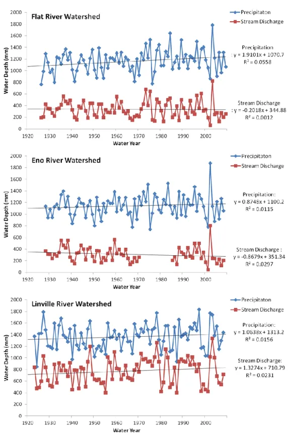
2.5.1 Precipitation and Stream Discharge trends
24
25
Figure 2.6: Examples precipitation and stream discharge trends of LULC conversion from
26 2.5.2 SWAT Calibration and validation
Figure 2.7, 2.8, 2.9 and Table 2.3 show calibration and validation results in the two Piedmont watersheds with LULC change and the Linville watershed. The number of simulation realizations for calibration and validation is 2000 each. Out of the 2000 simulations, the best simulated parameter sets are selected using a threshold NSE value of 0.5 for both NSE of stream discharge and
27
Table 2.3: Daily scale calibration and validation results of three study watersheds by Nash-Sutcliff Efficiency (NSE) of stream discharge (Q). Calibration and validation period are two years each
Flat River watershed Eno River watershed Liville River watershed
Best result (NSE_Q / NSE_logQ)
Calibration (1998-1999)
Validation (1996-1997)
Calibration (1998-1999)
Validation (1996-1997)
Calibration (1990-1991)
Validation (1992-1993)
28
29
30
31 2.5.3 Water year scale SWAT simulation since 1920
32
33
Table 2.4: Monthly scale SWAT simulation best result of three study watersheds by Nash-Sutcliff Efficiency (NSE) of stream discharge (Q) from 1986 to 2009.
Monthly (1986~2009) Flat River watershed Eno River watershed Liville River watershed
Best simulation result
34
35 2.5.4 Monthly scale stream discharge residual analysis
36
37
38 2.5.5 SWAT simulation with 1955 LULC
Using the same calibration and validation process as with NLCD 2006-based SWAT simulations, the Flat River watershed was simulated with 1955 LULC derived from aerial
photographs. Since LULC in 1955 contained more agricultural and less forested land than 2006 LULC, we expect that SWAT residual bias pattern with 1955 LULC would be different from SWAT residual bias pattern with 2006 LULC. In other words, if the under-predicted bias of SWAT with 2006 LULC in 1927 – mid-1970 is due to the amount of forested land, this bias could be mitigated with SWAT simulation with 1955 LULC.
Figure 2.13 is the result of SWAT simulations for the Flat River watershed with 1955 LULC with NSE of Q = 0.82 and NSE of logQ = 0.81 at monthly time scales as one of the best simulated result. The stream discharge difference between USGS and SWAT with the 1955 LULC shows a different trend compared with the SWAT simulations using the 2006 LULC. The water year scale SWAT with 1955 LULC shows a better fit to USGS measured stream discharge from 1927 to mid 1970’s, whereas simulated stream discharge became significantly higher than USGS measurements after the mid-1990’s. This pattern suggests that 1955 LULC, i.e. less forest and more
39
40
2.5.6 SWAT simulation differences between 1955 and 2006 LULC
Detailed SWAT simulated hydrologic components analysis explains the differences in hydrologic condition between 1955 and 2006 LULC in the Flat River watershed (Figure 2.14). In SWAT, total water yield (WY) as stream flow from each HRU is the sum of runoff from surface, shallow aquifer, and lateral flow from soil profile, and subtraction of transmission loss from channel bed and pond extraction. The transmission loss was excluded in this water balance analysis because it is so small, less than 1mm a month, and pond extraction was not considered in Flat River
41
42
43 2.6 Discussion
SWAT simulations for watersheds in the northern Piedmont of North Carolina experiencing forest re-growth show significant bias in the early decades of simulations assuming constant LULC, and not accounting for forest re-growth. This suggests that if current canopy cover existed through the full time period, this area would have produced less water yield than the actual, i.e., more agricultural, LULC condition. This bias is largely absent by the mid-1970’s, consistent with the approach of watershed conditions to current LULC. As simulated hydrographs are produced by measured historical weather conditions, i.e., precipitation and temperature, it can be assumed that the difference between simulated and measured stream discharge in the Flat and Eno River
watersheds is due to the LULC change.
44
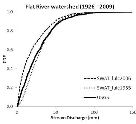
In order to analyze the change in three month for the purpose of water resources management in forest re-growth watershed, three month moving average monthly stream discharge of the Flat River watershed simulated by SWAT is presented as a cumulative distribution function (CDF). Figure 2.15 shows the CDFs in 1926 – 2009 of 1) USGS stream discharge, which represents stream discharge with historical LULC change by forest re-growth, 2) SWAT with lulc2006, which means simulated stream discharge with the static forest condition of 2006, and 3) SWAT with lulc1995, which implies simulated stream discharge with the static LULC condition as more agricultural land and less forest cover than 2006. SWAT with lulc2006 produces least amount of stream discharge, and SWAT with lulc1955 tends to simulate more stream discharge than SWAT with lulc2006 except extremely high stream discharge. USGS stream discharge tends to take its position between SWAT with lulc 2006 and SWAT with lulc1955 in below average stream discharge (i.e, CDF less than 0.5 level), which implies stream discharge condition by LULC transition from agricultural to forested cover. The high flow statistics, especially extreme high flow (i.e., CDF greater than 0.95 level) seems not to show significant variation between simulated and USGS stream discharge comparing with low flow portion. This result indicates that the effect of forest re-growth on water resources management needs to be more weighted to low flow than high flow period.
45
46 2.7 Conclusion
The simulations and analysis presented in this paper suggest that the lack of a definitive trend of increasing annual stream discharge of the Flat and the Eno River watersheds in the North Carolina Piedmont may be due to the offsetting impacts of increasing precipitation and forest re-growth. In the past with greater agricultural area, the runoff ratio of this region was higher than that of current forested conditions; less precipitation and more stream discharge in the past, compared with current more precipitation though with similar water yields as the past. This fact is confirmed by SWAT scenario simulations over the past century, which suggests that forested areas produce less water than agricultural areas in Piedmont with drier weather conditions similar to those of the past. As forests re-grow in abandoned agricultural fields, evapotranspiration gradually increases, especially during the vegetation growing season in spring and summer. If increasing vegetation water consumption is combined with less precipitation during the growing season, water shortage problem may be exacerbated. As a result, increasing water consumption by increasing forest water use may contribute to recent trends in hydrologic drought in the North Carolina Piedmont.
47
References
Abbaspour KC, 2011. SWAT-CUP4: SWAT Calibration and Uncertainty Programs – A User Manual. Eawag: Swiss Federal Institute of Aquatic Science and technology.
Andreadis K, Lettenmaier D, 2006. Trends in 20th century drought over the continental United States. Geophys.Res.Lett. ;33(10):L10403.
Arnold J, Srinivasan R, Muttiah R, Williams J, 1998. Large area hydrologic modeling and assessment - Part 1: Model development. J.Am.Water Resour.Assoc. ;34(1):73-89.
Beven K, Binley A, 1992. The Future of Distributed Models - Model Calibration and Uncertainty Prediction. Hydrol.Process. ;6(3):279-298.
Billings WD, 1938. The structure and development of old field shortleaf pine stands and certain associated physical properties of the soil. Ecol.Monogr. ;8:437-500.
Bosch,J . M., and J. D. Hewlett, 1982. A review of catchment experiments to determine the effect of vegetation changes on water yield and evapotranspiration. J,. Hydrol.,55, 3-23.
Buttle, J.M, 2011. Streamflow response to headwater reforestation in the Ganaraska River basin, southern Ontario, Canada. Hydrol.Process. ; 25:3030-3041
Center for Geographic Information and Analysis, 1:24,000 stream network data. http://www.cgia.state.nc.us/
Christensen N, Peet RR, 1984. Convergence during Secondary Forest Succession. J.Ecol. ;72(1):25-36. Farley K, Jobbagy E, Jackson R, 2005. Effects of afforestation on water yield: a global synthesis with implications for policy. Global Change Biol. ;11(10):1565-76.
Freer J, Beven K, Ambroise B, 1996. Bayesian estimation of uncertainty in runoff prediction and the value of data: An application of the GLUE approach RID C-7335-2009. Water Resour.Res.
;32(7):2161-73.
Hibbert, A.R., 1967. Forest treatment effects on water yield. In: W.E. Sopper and H.W. Lull (Editors), Int. Symp. For. Hydrol., Pennsylvania, September 1965. Pergamon, Oxford.
Huxman TE, Wilcox BP, Breshears DD, Scott RL, Snyder KA, Small EE, et al, 2005. Ecohydrological implications of woody plant encroachment. Ecology ;86(2).
Lins HF, Slack JR, 2005. Seasonal and regional characteristics of US streamflow trends in the United States from 1940 to 1999. Phys.Geogr. ;26(6):489-501.
48
Neitch SL, Arnold JG, Kiniry JR, Williams JR, 2011. Soil and Water Assessment Tool Theoretical Documentation Version 2009. Texas Water Resources Institute Technical Report No. 406, Texas A&M University System, College Station, Texas, USA.
National Oceanic and Atmospheric Administration (NOAA) Satellite and Information Service, Drought indices. http://www.ncdc.noaa.gov
Oosting H J, 1942. An ecological analysis of the plant communities of Piedmont, North Carolina, Amer Midland Nat, 28, 1-126.
Schilling KE, Libra RD, 2003. Increased baseflow in Iowa over the second half of the 20th century. J.Am.Water Resour.Assoc. ;39(4).
Schilling KE, Libra RD, 2003. Increased baseflow in Iowa over the second half of the 20th century. J.Am.Water Resour.Assoc. ;39(4).
Scott DF, Smith RE, 1997. Preliminary empirical models to predict reductions in total and low flows resulting from afforestation. Water Sa ;23(2).
Scott R, Huxman T, Williams D, Goodrich D, 2006. Ecohydrological impacts of woody-plant
encroachment: seasonal patterns of water and carbon dioxide exchange within a semiarid riparian environment. Global Change Biol. ;12(2):311-24.
Small D, Islam S, Vogel R, 2006. Trends in precipitation and streamflow in the eastern US: Paradox or perception? RID A-8513-2008. Geophys.Res.Lett. ;33(3):L03403.
Spear R, Hornberger G, 1980. Eutrophication in Peel Inlet .2. Identification of Critical Uncertainties Via Generalized Sensitivity Analysis. Water Res. ;14(1):43-49.
Swank WT, Douglass JE, 1974. Streamflow Greatly Reduced by Converting Deciduous Hardwood Stands to Pine. Science ;185(4154).
The University of North Carolina at Chapel Hill Institute for the Environment, 2009. Climate Change Committee Report.
Trimble S, Weirich F, Hoag B, 1987. Reforestation and the Reduction of Water Yield on the Southern Piedmont since Circa 1940. Water Resour.Res. ;23(3):425-37.
USDA (U.S. Department of Agriculture), 1900 – 2007. Agricultural census data. http://www.agcensus.usda.gov/Publications/Historical_Publications/index.php USDA (U.S. Department of Agriculture), 1955. Aerial photos in 1955.
USGS (U.S. Geological Survey), USGS water data for North Carolina. http://waterdata.usgs.gov/nc/nwis
USGS (U.S. Geological Survey), National Elevation Dataset. http://ned.usgs.gov/
Chapter 3: Evaluation and bias correction of NARCCAP nested
General Circulation Models (GCMs) and Regional Climate Models
(RCMs) precipitation and temperature in North Carolina for
hydrologic model application
3.1 Abstract
50
(Widmann et al., 2003) was applied to precipitation bias, and Tmax and Tmin biases were corrected by Fourier functions. After applying bias correction methods, NARCCAP climate simulation outputs have significant reduction of seasonal biases in precipitation, Tmax and Tmin except for a few extreme events. Application of raw and bias-corrected NARCCAP to a hydrologic model, the Soil and Water Assessment Tool (SWAT) shows that SWAT with bias-corrected NARCCAP simulated more reliable stream discharge than SWAT with raw NARCCAP simulation. Therefore, though these bias correction methods still show some errors, especially with extreme events, bias corrected data can be more appropriately used for not only currents and future climate simulations but also hydrologic model application.
3.2 Introduction
The aim of this chapter is the evaluation and bias correction of dynamically downscaled climate model information required for watershed simulation in North Carolina. The performance of climate models to simulate current climate should be acceptable before using future climate
prediction output. Un-biased climate model data is pre-requisite for not only climate change studies but also further applications, such as watershed hydrologic modeling. A set of the nested global and regional circulation model (GCM-RCM) results from the North American Regional Climate Change Assessment Program (NARCCAP) with current time simulations, are selected for model evaluation and bias correction.
51
multiple models (Intergovermental Panel on Climate Change (IPCC), 2007). The Southeast US in particular is an area in which simulated climate information does not agree well with observed climate (Nigam and Ruiz-Barradas 2006). For example, simulated annual precipitation is too large, summertime wetness is much too high, and winter precipitation simulation is dry with some models. One of the possible reasons which make Southeast US challenging area for climate modeling is its geographical location (Sobolowski and Pavelsky, 2012); the climate of this region is affected by the different ocean sources (i.e., Gulf of Mexico and Atlantic Ocean) as well as by mountainous topography (i.e., Appalachian and Blue Ridge Mountains).
There are several reasons why GCMs have problems with simulating current climate and by extension, predicting future climate conditions. GCMs are generally composed of three-dimensional numerical simulations of the atmosphere, ocean and land surface, which are represented by
relevant dynamical and physical processes (Noguer et al., 1998; Li et al., 2010). There are inherent errors of GCMs in formulating dynamics of each of these sub-systems and also their interactions (Goddard et al. 2001; Koster et al. 2000).
Modeling results of surface energy balance in GCM tend to be biased. One of the major reasons for this bias is that there are significant uncertainties in land surface parameters about vegetation thermal heterogeneity (Nasonova et al. 2011). For instance, if surface temperature is positively biased, latent heat flux is underestimated (overestimated) in summer (winter), and sensible heat flux is overestimated (underestimated) in summer (winter) (Chen et al. 1997). Soil moisture affects vegetation root-zone available water as well as runoff. Therefore, this may also cause significant modeling problems in the Southeast US with dense vegetation cover.
52
and non-linear (Goddard et al. 2001). Moreover, even though we assume that SSTs could be simulated and predicted perfectly, chaotic atmospheric dynamics and limited land surface simulation can cause significant limits on precipitation simulation (Koster et al. 2000). Another serious problem about the interactions in atmosphere, sea, and land is that these three components have different time scales for mathematical formulation; i.e. a few days of atmosphere, and more than a couple of months or longer of ocean conditions (Goddard et al. 2001). So initializing of each component makes the models much more complex. Overall, the discrepancy between simulations and observations may be due to a number of reasons, such as neglected physical processes in the models, uncertainty about important parameter values, lack of detailed descriptions of the specific conditions, lack of atmospheric forcing data before the year that would allow appropriate spin-up, or the assumption that simulation results with coarse grid resolution, and simplification of the natural heterogeneity of the climate system that exist at finer spatial scales (Chen et al. 1997; Li et al., 2010).
53
Ensembles-Based Predictions of Climate Changes and Their Impacts (ENSEMBLES) program and the North American Regional Climate Change Assessment Program (NARCCAP) project (Themeβl et al., 2010).
However, RCMs could add additional error and uncertainty even though the largest sources of modeling uncertainties may be inherited from the driving GCM (Noguer et al., 1998; Fowler et al., 2007; de Elia et al., 2008). In RCM simulations, inadequate representations of local forcing, such as orography, land-sea contrast and vegetation cover, may still bring errors in the finer scale
simulations (Noguer et al., 1998; Fowler et al., 2007). For example, overestimated precipitation of RCM may be due to inaccurate parameterizations of large-scale condensation and convection schemes, poor soil parameterizations, lack of moisture advection into the region, or poor simulation of snow-albedo feedback (Fowler et al., 2007). Thus, regional systematic errors can be introduced by RCM physical processes to the GCM framework.
Other GCM downscaling tools are statistical methods which establish empirical relationships between GCM and local climate variables. In the review paper of Fowler et al. (2007), they classified and compared statistical downscaling methods in several groups, including change factors, simple analogue methods, regression models, weather typing schemes, and weather generators. They found that GCM precipitation considerably improved by simple statistical methods, a finding supported by other studies (Zortia and von Storch, 1999; Widmann et al., 2003; Schmidlie et al., 2006). As dynamical downscaling alone has not led to large improvements in bias relative to GCM output alone, a combination of dynamical and statistical approaches has been used to gain an improvement over their use alone (Diez et al., 2005).
54
present climate conditions (Wilby et al., 2000; Hay and Clark, 2003; Wilby and Wigley, 2000; Wood et al., 2004; Li et al., 2010). This is one of the reasons why statistical methods are widely used in climate impact related studies. However, the key weakness of statistical methods is the stationarity assumption in statistical models (Li et al., 2010). This weakness can be partially alleviated by specific statistical model application strategies. For example, Salathe (2003) divided time period on the basis of Pacific Decadal Oscillation (PDO) phase change for the scale factor application; 1958~1976 is downscaled with scale factors for data of 1977~1994 and vice versa. In this manner, the statistical model fitting process can reflect the effect of the shifts in the natural climate.
Not only NARCCAP bias correction alone, but also the applicability of NARCCAP to watershed hydrologic model is the goal of this study as well. Therefore, both raw and bias-corrected NARCCAP precipitation and temperature are applied to the Soil and Water Assessment Tool (SWAT) in one of the major water supply basins in the North Carolina Piedmont to compare the effect of raw and bias corrected NARCCAP to hydrologic modeling.
In this study, we pose the following questions:
1) Are systematic biases found in NARCCAP produced GCM-RCM daily precipitation, and maximum and minimum temperature in the North Carolina region?
2) If there are systematic biases, can we apply statistical methods to efficiently correct the biases?
3) Is bias correction of NARCCAP necessary for its application to hydrologic modeling? To what extent can bias corrected NARCCAP output improve hydrologic modeling
55 3.3 Methods
3.3.1 Evaluation of North American Regional Climate Change Assessment Program (NARCCAP) GCM-RCM precipitation and temperature
The North American Regional Climate Change Assessment Program (NARCCAP) is an
international program to produce high resolution climate change simulations in order to investigate uncertainties in regional scale projections of future climate and generate climate change scenarios for use in impacts research (http://www.narccap.ucar.edu). It provides a set of regional climate models (RCMs) driven by a set of atmosphere-ocean general circulation models (AOGCMs) over a domain covering the conterminous United States, most of the Canada, and northern Mexico. The AOGCMs in NARCCAP have been forced with the Special Report on Emission Scenario (SRES) (IPCC, 2000) A2 emissions scenario for the 21st century. SRES is the green house gas emission scenarios for future climate change. The A2 scenario is a worst-case scenario, in which CO2 emission over 2000-2099 will increase to be 350 – 850 ppm. It is based on an economic storyline with high population growth, regionally oriented economic development, and slow technological change. Simulations with the NARCCAP models were also produced for the current (historical) period. The RCMs are nested within the AOGCMs for 1971-2000 and for a future period 2041-2070.
A major advantage of NARCCAP output is the provision of daily time scale weather data. Since one of the main purposes of climate data evaluation and bias correction in this study is preparing input weather data for hydrologic models which requires daily weather input data, NARCCAP is one of the appropriate data sources for watershed hydrologic simulation.