Quantum phase estimation of multiple eigenvalues for small-scale (noisy) experiments

PAPER • OPEN ACCESS

Quantum phase estimation of multiple eigenvalues

for small-scale (noisy) experiments

To cite this article: Thomas E O’Brien et al 2019 New J. Phys. 21 023022

View the article online for updates and enhancements.

Recent citations

Random Compiler for Fast Hamiltonian Simulation

Earl Campbell

-Magnetic-Field Learning Using a Single Electronic Spin in Diamond with One-Photon Readout at Room Temperature

R. Santagati et al

-Accelerated Variational Quantum Eigensolver

Daochen Wang et al

PAPER

Quantum phase estimation of multiple eigenvalues for small-scale

(noisy) experiments

Thomas E O’Brien1,4

, Brian Tarasinski2

and Barbara M Terhal2,3

1 _{Instituut Lorentz, Universiteit Leiden, P.O. Box 9506, 2300 RA Leiden, The Netherlands} 2 _{QuTech, Delft University of Technology, P.O. Box 5046, 2600 GA Delft, The Netherlands}

3 _{JARA Institute for Quantum Information(PGI-11), Forschungszentrum Juelich, D-52425 Juelich, Germany} 4 _{Author to whom any correspondence should be addressed.}

E-mail:[email protected]

Keywords:quantum information, quantum algorithms, quantum phase estimation, digital quantum simulation

Abstract

Quantum phase estimation

(QPE)

is the workhorse behind any quantum algorithm and a promising

method for determining ground state energies of strongly correlated quantum systems. Low-cost QPE

techniques make use of circuits which only use a single ancilla qubit, requiring classical post-processing to

extract eigenvalue details of the system. We investigate choices for phase estimation for a unitary matrix

with low-depth noise-free or noisy circuits, varying both the phase estimation circuits themselves as well as

the classical post-processing to determine the eigenvalue phases. We work in the scenario when the input

state is not an eigenstate of the unitary matrix. We develop a new post-processing technique to extract

eigenvalues from phase estimation data based on a classical time-series

(or frequency)

analysis and contrast

this to an analysis via Bayesian methods. We calculate the variance in estimating single eigenvalues via the

time-series analysis analytically,

finding that it scales to

first order in the number of experiments

performed, and to

first or second order

(depending on the experiment design)

in the circuit depth.

Numerical simulations confirm this scaling for both estimators. We attempt to compensate for the noise

with both classical post-processing techniques,

finding good results in the presence of depolarizing noise,

but smaller improvements in 9-qubit circuit-level simulations of superconducting qubits aimed at

resolving the electronic ground state of a H4-molecule.

1. Introduction

It is known that any problem efficiently solvable on a quantum computer can be formulated as eigenvalue sampling of a Hamiltonian or eigenvalue sampling of a sparse unitary matrix[1]. In this sense the algorithm of quantum phase estimation(QPE)is the only quantum algorithm which can give rise to solving problems with an exponential quantum speed-up. Despite it being such a central component of many quantum algorithms, very little work has been done so far to understand what QPE in the current noisy intermediate scale quantum

(NISQ)era of quantum computing[2]where quantum devices are strongly coherence-limited. QPE comes in many variants, but a large subclass of these algorithms(e.g. the semi-classical version of textbook phase estimation[3,4], Kitaev’s phase estimation[5], Heisenberg-optimized versions[6]), are executed in an iterative sequential form using controlled-Ukgates with a single ancilla qubit[7,8](seefigure1), or by direct

measurement of the system register itself[6]. Such circuits are of practical interest in the near term when every additional qubit requires a larger chip and brings in additional experimental complexity and incoherence.

Some of the current literature on QPE works under limiting assumptions. Thefirst is that one does not start in an eigenstate of the Hamiltonian[9,10]. A second limitation is that one does not take into account the(high) temporal cost of runningUk[8]for largekwhen optimizing phase estimation. The size and shallowness of the QPE circuit is important since, in the absence of error correction or error mitigation, one expects entropy build-up during computation. This means that circuits with largekmay not be of any practical interest.

OPEN ACCESS

RECEIVED 31 October 2018

REVISED 17 December 2018

ACCEPTED FOR PUBLICATION 2 January 2019

PUBLISHED 28 February 2019

Original content from this work may be used under the terms of theCreative Commons Attribution 3.0 licence.

Any further distribution of this work must maintain attribution to the author(s)and the title of the work, journal citation and DOI.

The scenario where the input state is not an eigenstate of the unitary matrix used in phase estimation is the most interesting one from the perspective of applications, and we will consider it in this work. Such an input state can be gradually projected onto an eigenstate by the phase estimation algorithm and the corresponding eigenvalue can be inferred. However, for coherence-limited low-depth circuits one may not be able to evolve sufficiently long to project well onto one of the eigenstates. This poses the question what one can still learn about eigenvalues using low-depth circuits. An important point is that it is experimentally feasible to repeat many relatively shallow experiments(or perform them in parallel on different machines). Hence we ask what the spectral-resolving power of such phase estimation circuits is, both in terms of the number of applications of the controlled-Ucircuit in a single experiment, and the number of times the experiment is repeated. Such repeated phase estimation experiments require classical post-processing of measurement outcomes, and we study two such algorithms for doing this. One is our adaptation of the Bayesian estimator of[10]to the multiple-eigenvalue scenario. A second is a new estimator based on a treatment of the observed measurements as a time-series, and construction of the resultant time-shift operator. This latter method is very natural for phase estimation, as one interprets the goal of phase estimation as the reconstruction of frequencies present in the output of a temporal sound signal. In fact, the time-series analysis that we develop is directly related to what are called Prony-like methods in the signal-processing literature, see e.g.[11]. The use of this classical method in quantum signal processing, including in quantum tomography[12], seems to hold great promise.

One can interpret our results as presenting a new hybrid classical-quantum algorithm for QPE. Namely, when the number of eigenstates in an input state is small, i.e. scaling polynomially with the number of qubitsnsys, the use of our classical post-processing method shows that there is no need to run a quantum algorithm which projects onto an eigenstate to learn the eigenvalues. We show that one can extract these eigenvalues efficiently by classically post-processing the data from experiments using a single-round QPE circuits(see section2)and classically handling

n n

poly( sys)´poly( sys)matrices. This constitutes a saving in the required depth of the quantum circuits.

The spectral-resolution power of QPE can be defined by its scaling with parameters of the experiment and the studied system. We are able to derive analytic scaling laws for the problem of estimating single eigenvalues with the time-series estimator. Wefind these to agree with the numerically-observed scaling of both studied estimators. For the more general situation, with multiple eigenvalues and experimental error, we study the error in estimating the lowest eigenvalue numerically. This is assisted by the low classical computation cost of both estimators. We observe scaling laws for this error in terms of the overlap between the ground and starting state

(i.e. the input state of the circuit), the gap between the ground and excited states, and the coherence length of the system. In the presence of experimental noise we attempt to adjust our estimators to mitigate the induced estimation error. For depolarizing-type noise wefind such compensation easy to come by, whilst for a realistic circuit-level simulation wefind smaller improvements using similar techniques.

Even though our paper focuses on QPE where the phases corresponds to eigenvalues of a unitary matrix, our post-processing techniques may also be applicable to multi-parameter estimation problems in quantum optical settings. In these settings the focus is on determining an optical phase-shift[13–15]through an interferometric set-up. There is experimental work on(silicon)quantum photonic processors[16–18]on multiple-eigenvalue estimation for Hamiltonians which could also benefit from using the classical post-processing techniques that we develop in this paper.

Figure 1.Circuit for the QPE experiments described in this work. The state∣Yñis defined in equation(3). The probability for the ancilla qubit to return the vectormof results in the absence of error is given by equation(10). The single-qubit rotation equals

Z exp i 2

z

2. Quantum phase estimation

QPE covers a family of quantum algorithms which measure a system register ofnsysqubits in the eigenbasis of a unitary operatorU[5,19]

U_∣f_jñ =eifj_∣f_jñ, _{( )}1

to estimate one or many phasesfj. QPE algorithms assume access to a noise free quantum circuit which implementsUon our system register conditioned on the state of an ancilla qubit. Explicitly, we require the ability to implement

U

0 0 1 1 , 2

c

 = ñá Ä + ñá Ä∣ ∣  ∣ ∣ ( )

where∣0ñand∣1ñare the computational basis states of the ancilla qubit, andis the identity operator on the system register.

In many problems in condensed matter physics, materials science, or computational chemistry, the object of interest is the estimation of spectral properties or the lowest eigenvalue of a Hamiltonian. The eigenvalue estimation problem forcan be mapped to phase estimation for a unitaryUt=exp(-it)with aτchosen

such that the relevant part of the eigenvalue spectrum induces phases within[−π,π). Much work has been devoted to determining the most efficient implementation of the(controlled)-exp(-it)operation, using exact or approximate methods[19–22]. Alternatively, one may simulatevia a quantum walk, mapping the problem to phase estimating the unitaryexp(-iarcsin() l)for someλ, which may be implemented exactly

[23–26]. In this work we do not consider such variations, but rather focus on the error in estimating the eigenvalue phases of the unitaryUthat is actually implemented on the quantum computer. In particular, we focus on the problem of determining the value of a single phasef0to high precision(this phase could

correspond, for example, to the ground state energy of some Hamiltonian). Phase estimation requires the ability to prepare an input, orstarting state

a ,A a , 3

j

j j j j2

å

Yñ = ñ º

∣ ∣ ∣ ∣ ( )

with good overlap with the ground state;A0?0. Note here that the spectrum ofUmay have exact degeneracies

(e.g. those enforced by symmetry)which phase estimation does not distinguish; we count degenerate eigenvalues as a singlefjthroughout this work. The ability to start QPE in a state which already has good overlap with the ground state is a non-trivial requirement for the applicability of the QPE algorithm. On the other hand, it is a well-known necessity given the QMA-completeness[27]of the lowest eigenvalue problem5. For many quantum chemistry and materials science problems it is known or expected that the Hartree–Fock state has good overlap with the ground state, although rigorous results beyond perturbation theory are far and few between(see e.g.

[28]). Beyond this, either adiabatic evolution[20,29]or variational quantum eigensolvers[30]can provide an approximate starting state to improve on via phase estimation.

Phase estimation is not limited to simply learning the value off0; it may obtain information about all phases fjas long asAj>0. However, the resources required to estimatef_jare bounded below by 1/Aj. To see this, note that the controlled-unitarycdoes not mix eigenstates, and so there is no difference(in the absence of error)

between starting with∣Yñand the mixed state

A . 4

j

j j j

å

r_Y= ∣f fñá ∣ ( )

The latter is then equivalent to preparing the pure state∣f_jñwith probabilityAj, so ifNpreparations of∣f_jñare required to estimatefjto an errorò, the same error margin requires at leastN/Ajpreparations of the state∣Yñ. As the number of eigenstatesNeigwith non-zero contribution to∣Yñgenerally scales exponentially with the system sizensys, estimating more than thefirst fewfj(ordered by the magnitudeAj)will be unfeasible.

Low-cost(in terms of number of qubits)QPE may be performed by entangling the system register with a single ancilla qubit[5,8,10,27]. Infigure1, we give the general form of the quantum circuit to be used throughout this paper. An experiment, labeled by a numbern=1,K,N, can be split into one or multiple roundsr=1,K,Rn, following the preparation of the starting state∣Yñ. In each round a single ancilla qubit prepared in the 1 0 1

2

+ñ = ñ + ñ

∣ (∣ ∣ )state controls_ckr_{where the integerk}

rcan vary per round. The ancilla qubit is then rotated byz( )br =exp(-ibrZ 2)(with the phaseβrpossibly depending on other rounds in the same experiment)and read out in theX-basis, returning a measurement outcomemrä{0, 1}. We denote the 5

chosen strings of integers and phases of a single multi-round experiment bykandb, respectively. We denote the number of controlled-Uiterations per experiment asK= å_rR=n1kr. We denote the total number of controlled-U

iterations over all experiments as

K k. 5

n N

r R

r

tot

1 1

n

å å

= =

( )

As the system register is held in memory during the entire time of the experiment, the choice ofKis dictated by the coherence time of the underlying quantum hardware. Hence, we introduce a dimensionless coherence length

K T

n TU. 6

err err sys

= ( )

HereTUis the time required to implement a single application of controlled-Uin equation(7), andTerris the

time-to-error of a single qubit, so thatTerr nsysis the time-to-failure ofnsysqubits. The idea is thatKerrbounds

the maximal number of applications ofUin an experiment, namelyK„Kerr.

A new experiment starts with the same starting state∣Yñ. Values ofkrandβrmay be chosen independently for separate experimentsn, i.e. we drop the labelnfor convenience. We further drop the subscriptrfrom single-round experiments(withR=1).

In the absence of error, one may calculate the action of the QPE circuit on the starting state(defined in equation(3)). Working in the eigenbasis ofUon the system register, and the computational basis on the ancilla qubit, we calculate the state following the controlled-rotation_ck1_{, and the rotation}

z 1

 ( )b on the ancilla qubit to be

a

1

2 j 0 e 1 . 7

j ik1 j 1 j

å

The probability to measure the ancilla qubit in theX-basis asm1ä{0, 1}is then

A cos k m

2 2 , 8

j j

j

2 1 1 1

å

⎝

⎜ ⎞

⎠

⎟ ( )

and the unnormalized post-selected state of the system register is

ae cos k m

2 2 . 9

j j k

j

j

1 _{1 1}

j

i 2 1 1

å

⎝

⎜ ⎞

⎠

⎟∣ ( )

( )

The above procedure may then be repeated forrrounds to obtain the probability of a stringmof measurement outcomes of one experiment as

P m ,A A cos k m

2 2 . 10

j j

r R

r j r r

k,

1 2

å 

f = f + b - p

b

=

⎛ ⎝

⎜ ⎞

⎠ ⎟

( ∣ ) ( )

Here,fis the vector of phasesfjandAthe vector of probabilities for different eigenstates. We note that

Pk,b( ∣mf,A)is independent of the order in which the rounds occur in the experiment. Furthermore, when

Neig=1,Pk,b( ∣ )mf =Pk,b( ∣mf,A)is equal to the product of the single-round probabilitiesPkr,br(mr∣ ), as theref

is no difference between a multi-round experiment and the same rounds repeated across individual experiments. One can make a direct connection with parameter estimation work by considering the single-round

experiment scenario infigure1. The Hadamard gate putting the ancilla qubit in∣+ñand measuring the qubit in the

X-basis are, in the optical setting, realized by beam-splitters, so that only the path denoted by the state∣1ñwill pick up an unknown phase-shift. When the induced phase-shift is not unique but depends, say, on the state of another quantum system, we may like to estimate all such possible phases corresponding to our scenario of wishing to estimate multiple eigenvalues. Another physical example is a dispersively coupled qubit-cavity mode system where the cavity mode occupation number will determine the phase accumulation of the coupled qubit[31].

3. Classical data analysis

Two challenges are present in determiningf0from QPE experiments. First, we only ever have inexact sampling

knowledge ofPk,b( ∣mf,A). That is, repeated experiments atfixedk,bdo not directly determine

Pk,b( ∣mf,A), but rather sample from the multinomial distributionPk,b( ∣mf,A). From the measurement outcomes we can try to estimatePk,b( ∣mf,A)(and from thisf0)as a hidden variable. Secondly, whenNeig>1 determiningf0fromPk,b( ∣mf,A)poses a non-trivial problem.

Let usfirst consider the caseNeig=1. Let us assume that we do single-round experiments with afixedkfor each experiment. Naturally, takingk=1 would give rise to the lowest-depth experiments. If we start these experiments withk=1 in the eigenstate∣f₀ñ, then one can easily prove that takingβ=0 or

2

bounds, see e.g.[32,33], and represent standard sampling or shot noise behavior. WhenNeig=1,N K-round experiments each withk=1 are indistinguishable fromN×Ksingle-round experiments withk=1. This implies that the same scaling holds for such multi-round experiments, i.e. the variance scales as1 (NK)=1 Ktot.

Once the phasef0is known to sufficient accuracy, performing QPE experiments withk>1 is instrumental in

resolvingf0in more detail, since the probability of a single-round outcome depends onkf0[6]. Once one knows with

sufficient certainty thatf₀Î[(2m-1)p k, 2( m+1)p k)(for integerm), one can achieve variance scaling as k N

1_/ 2 _{(conforming to so-called local estimation Cramer–Rao bounds suggested in[10,34]). A method achieving} Heisenberg scaling, where the variance scales as1/Ktot2 (see equation(5)), was analyzed in[6,32]. This QPE method can also be compared with the information-theoretic optimal maximum-likelihood phase estimation method of[8]

whereN~logKexperiments are performed, each choosing a randomkÎ{1,¼,K}to resolvef0with error

scaling as 1/K. The upshot of these previous results is that, while the variance scaling in terms of the total number of unitaries goes like 1/Ktotwhen usingk=1, clever usage ofk>1 data can lead to1 Ktot2 scaling. However, asKis limited byKerrin near-term experiments, this optimal Heisenberg scaling may not be accessible.

WhenNeig>1, the above challenge is complicated by the need to resolve the phasef0from the otherfj.

This is analogous to the problem of resolving a single note from a chord. Repeated single-round experiments at

fixedkand varyingβcan only give information about the value of the function:

g k Ae , 11

j j ik j

å

= f

( ) ( )

at thisfixedk, since

P m m g k

m g k

1 2

1

2cos Re

1

2sin Im . 12

k, f b p

b p

= + +

- +

b( ∣ ) ( ) [ ( )]

( ) [ ( )] ( )

This implies that information from single-round experiments atfixedkis insufficient to resolvef0whenNeig>1, asg(k)is then not an invertible function off0(try to recover a frequency from a sound signal at a single point in

time!). In general, for multi-round experiments using a maximum ofKtotal applications ofc, we may only ever

recoverg(k)fork„K. This can be seen from expandingPk,b( ∣mf,A)as a sum ofåjAjcosm( )fj sinn( )fj terms

withm+n„K, which are in turn linear combinations ofg(k)fork„K. As we will show explicitly in the next section3.1this allows us to recover up toKfj. However, whenNeig>K, these arguments imply that we cannot recover any phases exactly. In this case, the accuracy to which we can estimate our targetf0is determined by the

magnitude of the amplitudeA0in the inital state∣Yñas well as the gap towards the other eigenvalues. For example,

in the limitA0 1, an unbiased estimation off0using data fromk=1 would be

g A

Arg 1 Im ln e , 13

j j i j

å

= ⎡ f

⎣ ⎢ ⎢

⎛

⎝

⎜⎜ ⎞_⎠⎟⎟⎤

⎦ ⎥ ⎥

[ ( )] ( )

and the error in such estimation is

g

A A O A

A A

Arg 1 1 sin

1 ,

j N

j j

0

0 1 1

0 02

0

0

eig



å

f f f

- = - +

-=

-∣ [ ( )] ∣ ( ) ( )

with our bound being independent ofNeig. We are unable to extend this analysis beyond thek=1 scenario, and instead we study the scaling in this estimation numerically in section4. In the remainder of this section, we present two estimators for multi-round QPE. Thefirst is an estimator based on a time-series analysis of the functiong(k)using Prony-like[11]methods that has a low computation overhead. The second is a Bayesian estimator similar to that of[10], but adapted for multiple eigenphasesfj.

3.1. Time-series analysis

Let us assume that the functiong(k)in equation(11)is a well-estimated function at all points 0„k„K, since the number of experimentsNis sufficiently large. We may extend this function to all points-K k Kusing the identityg(-k)=g k*( )to obtain a longer signal6. We wish to determine the dominant frequenciesfjin the signalg(k)as a function of‘time’k. This can be done by constructing and diagonalizing a time-shift matrixT whose eigenvalues are the relevant frequencies in the signal, as follows.

6

Wefirst demonstrate the existence of the time-shift matrixTin the presence ofNeig<K

separate frequencies. Since we may not knowNeig, let usfirst estimate it asl. We then define the vectors

k g k g k g k l

g_{( )=( ( )}, _{( +}1 ,_{)¼ ( + ))}T_{,k= -K,¼,K. These vectors can be decomposed in terms of}

single-frequency vectorsbj=(1, e ,ifj ¼, eilfj)T

k A

g e b. 14

j

j ik j j

å

= f

( ) ( )

We can make al´NeigmatrixBwith the componentsbjas columns

Bk j, =eikfj. (15)

WhenNeigl, the columns ofBare typically linearly independent7, hence the non-square matrixBis invertible

and has a(left)-pseudoinverseB−1such thatB−1B=1. Note however, whenNeig>lthe columns ofBare

linearly-dependent, soBcannot be inverted. IfBis invertible, we can construct the shift matrix_T=BDB-1 withDi,j=di,jeifj. By construction,Tb_j=eifjb_j(asTB=BD), and thus

k A

A k

g b

g e

e 1 . 16

j

j k j

j j k

i

i 1

j

j

å

å

= = +

f

f +

( )

( ) ( )

( )

T T

This implies thatTacts as the time-shift operator mappingg(k)tog(k+1). As the eigenvalues ofTare precisely the required phaseseifjin caseN_eigl, constructing and diagonalizingTwill obtain our desired phases

includingf0. WhenNeig>l, the eigen-equation forTcannot have the solutionbjsince these are not linearly independent.

The above proof of existence does not give a method of constructing the time-shift operatorT, as we do not have access to the matricesBorD. To constructTfrom the data that we do have access to, we construct the

l´(2K+ -1 l)Hankel matricesG(0),G(1)by

G_{i j}( )_,a =g i( + + -j a K), (17)

indexing 0„i„l−1,0 j 2K-l. Thekth column ofG(a)is the vectorg(k+ -a K), and so

G( )0 ₌G( )1

T . We can thus attempt tofindTas a solution of the(least-squares)problem of minimizing

G0 _-G1

∣∣_T ( ) ( )∣∣_{. The rank of the obtainedT˜is bounded by the rank ofG}(0)

. We have thatrank₍G( )0_{)is at most} Neigsince it is a sum over rank-1 matrices. At the same timerank(G( )0)min , 2(l K+ -1 l). This implies that we require bothlNeigand2K+ -1 lNeigto obtain a shift matrixTwithNeigeigenvalues. This is only possible whenKNeig, giving an upper bound for the number of frequencies obtainable. WhenG(0)is not full rank(becauseNeig<l), this problem may have multiple zerosT. However, when˜ Neig<leach of these must satisfyT˜ ( )gk =g(k+1)for- < <K k K-l.

Then, as long asrank G0 N

eig 

( ( )) _{, equation(14)is invertible by an operatorC}

C A e b C g k. 18

k

i k j k i j j k

j k

, i j , ,

å

å

It follows that

C gk 1 C Ae e b e b, 19

k j k

k l

j k l k l j

,

,

, i l i l i j

å

å

and then

C k C k

bj g g 1 e b, 20

k k j

k

k j j

, , i j

å

å

= = + = f

˜ _{˜ ( ) ( ) ( )}

T T

so everyT˜obtained in this way must have eigenvalueseifj.

The above analysis is completely independent of the coefficientsAj. However, once the eigenvaluesfjare known, the matrixB(equation(15))may be constructed, and theAjmay be recovered by a subsequent least-squares minimization of

BA-g 0 . 21

∣∣ ( )∣∣ ( )

This allows us to identify spurious eigenvalues ifl>Neig(as these will have a corresponding zero amplitude). Numerically, wefind no disadvantage to then choosing the largestlpermitted by our data, namelyl=K. 7

Assuming a sufficient number of repetitionsNthese arguments imply that this strategy requires that

KNeigto determine all eigenvalues accurately. However, whenK<Neigthere still exists a least-squares solutionT˜that minimizes_{∣∣ ˜T}G( )0 _-G( )1_{∣∣. WhenA}

0?1/K, we expect thatT˜ should have eigenvalues

eif˜0»eif0that we can take as the estimator forf₀; the same is true for any otherf_jwith sufficiently largeA_j. In

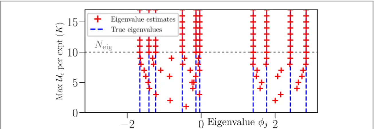
figure2we show an example of convergence of this estimation for multiple eigenvaluesf_jasKNeigin the case whereg(k)is known precisely(i.e. in the absence of sampling noise). The error∣ ˜f₀-f₀∣whenK<Neig depends on the eigenvalue gap abovef0, as well as the relative weightsAj, as we will see in section4.3.

In appendixBwe derive what variance can be obtained with this time-series method in the case

l=Neig=1, using single-round circuits withk=1 up toK. Our analysis leads to the following scaling inNandK:

K N

Var 1 . 22

2 f µ

( ) ( )

We will compare these results to numerical simulations in section4.1.

3.1.1. Estimatingg(k)

The functiong(k)cannot be estimated directly from experiments, but may instead be created as a linear

combination ofPk,b( ∣mf,A)for different values ofkandβ. For single-round experiments, this combination is simple to construct:

g k P P

P P

A A

A A

0 , 1 ,

i 0 , i 1 , . 23

k k

k k

,0 ,0

,2 ,2

f f

f f

=

-- p + p

( ) ( ∣ ) ( ∣ )

( ∣ ) ( ∣ ) ( )

For multi-round experiments, the combination is more complicated. In general,Pk,b( ∣mf,A)is a linear combination of real and imaginary parts ofg(l)withl<K= å_rkr. This combination may be constructed by

writingcos2₍k_fj 2_+b 2_{)andsin k 2 2}

j

2_{( f +b )in terms of exponentials, and expanding. However,} inverting this linear equation is a difficult task and subject to numerical imprecision. For somefixed choices of experiments, it is possible to provide an explicit expansion. Here we focus onK-roundk=1 experiments with

K/2β=0 andK/2 2

b= pfinal rotations during each experiment(choosingKeven). The formula for

Pk,b( ∣mf,A)is independent of the order in which these rounds occur. Let us write(m n, ∣f,A)as the probability of seeing bothmÎ{0,¼,K 2}outcomes withmr=1 in theK/2 rounds withβr=0 and

K

0, , 2

Î{ ¼ }

n outcomes withnr=1 in theK/2 rounds withβr=π/2. In other words,m,nare the Hamming weights of the measurement vectors split into the two types of rounds described above. Then, one can prove that, for 0„k„K/2:

g k , , ,A , 24

m K

n K

k

0 2

0 2



å å

=

= =

( ) (m n) (m n∣ ) ( )

Figure 2.Convergence of the time-series estimator in the estimation ofNeig=10eigenvalues(chosen at random with equally sized

where

i k

l

,

1

1 . 25

k

l k

k l

p

l _p K_{l p}

K l

p

k l _{p k}K _{l p}

K k l

0

0

2 ₂ 2₂

2

0

2 ₂ 2 ₂

2 1 1 1 2 2 2

å

å

å

c =

-´ -´ -= -= -= - _{- -} -⎜ ⎟ ⎛ ⎝ ⎞ ⎠ ⎡ ⎣ ⎢ ⎢ ⎢ ⎤ ⎦ ⎥ ⎥ ⎥ ⎡ ⎣ ⎢ ⎢ ⎢ ⎤ ⎦ ⎥ ⎥ ⎥

( )(

)

( )(

)

( )

( )

The proof of this equality can be found in appendixA.

Calculatingg(k)from multi-round(k=1)experiments contains an additional cost: combinatorial factors in equation(24)relate the variance ing(k)to the variance in(m n, ∣f,A)but the combinatorial pre-factor k l ⎜ ⎟ ⎛ ⎝ ⎞ ⎠ can increase exponentially ink. This can be accounted for by replacing the least squaresfit used above with a weighted least squaresfit, so that one effectively relies less on the correctness ofg(k)for largek. To do this, we construct the matrixTrow-wise from the rowsg_i( )1 _ofG(1)_{. That is, for theith row}

i

t we minimize

G g . 26

i 0 - _i1

∣∣_t ( ) ( )∣∣ ( )

This equation may be weighted by multiplyingG(0)andg_i( )1 _{by the weight matrix}

w_{j k}i j k 1 , 27

G

, ,

i j, 1 d s = ( ) ( ) ( ) where _G

i j, 1

s ( )is the standard deviation in our estimate ofG i j,

1

( )_{. Note that the method of weighted least-squares is}

only designed to account for error in the independent variable of a least squaresfit, in our case this isG(1). This enhanced effect of the sampling error makes the time-series analysis unstable for largeK. We can analyze how this weighting alters the previous variance analysis whenNeig=1. If we take this into account(see derivation in appendixB), wefind that

KN

Var( )f µ 1 , (28)

for a time-series analysis applied to multi-roundk=1 experiments.

3.1.2. Classical computation cost

In practice, the time-series analysis can be split into three calculations;(1)estimation ofPk,b( ∣mf,A)or A

, ,

(m n∣f ),(2)calculation ofg(k)from these probabilities via equation(23)or equation(24), and

(3)estimation of the phasesffromg(k). Clearly(2)and(3)only need to be done once for the entire set of experiments.

The estimation of the phasesfrequires solving two least squares equations, with costO l K₍2 _{)(recalling thatl} is the number of frequencies to estimate, andKis the maximum known value ofg(k)), and diagonalizing the time-shift matrixTwith costO(l3). For single-round phase estimation this is the dominant calculation, as calculatingg(k)from equation(23)requires simplyKadditions. As a result this estimator proves to be incredibly fast, able to estimate one frequency from a set ofN=106experiments of up toK=10 000 in<100 ms, and

l=1000 frequencies fromN=106experiments withK=1000 in<1 min. However, for multi-round phase estimation the calculation ofg(k)in equation(24)scales asO(K4). This then dominates the calculation, requiring 30 s to calculate 50 points ofg(k).(All calculations performed on a 2.4 GHz Intel i3 processor.)We note that all the above times are small fractions of the time required to generate the experimental data whenN?K, making this a very practical estimator for near-term experiments.

3.2. Efficient Bayesian analysis

When the starting state is the eigenstate∣f₀ñ, the problem of determiningf0based on the obtained

multi-experiment data has a natural solution via Bayesian methods[10,35]. Here we extend such Bayesian methodology to a general starting state. For computational efficiency we store a probability distribution over phasesP(f)using a Fourier representation of this periodic functionP(f) (see appendixC). This technique can also readily be applied to the case of Bayesian phase estimation applied to a single eigenstate.

m_{i i}N

1

=

{ } , one can simply chooseA,fwhich maximizes the posterior distribution:

P P

P P

A m A

m A

, i , , , 29

i k post , prior i i

f = b f f

( ) ({ }∣ )

({ }) ( ) ( )

{ } { }

In other words, one chooses

P

P P

A A

m A A

, arg max log ,

arg max log i , log , .

A A k

opt opt

, post

, i, i prior

f f f f = = + f f b ( ) ( ) [ { } { }({ }∣ ) ( )]

A possible way of implementing this strategy is to(1)assume the prior distribution to be independent ofAandf and(2)estimate the maximum by assuming that the derivative with respect toAandfvanishes at this

maximum.

Instead of this method we update our probability distribution overfandAafter each experiment. After experimentnthe posterior distributionPn(f,A)via Bayes’rule reads

P P

P P

A m A

m A

, , , . 30

n f k, n 1

f

f

= b

-( ) ( ∣ )

( ) ( ) ( )

To calculate the updates we will assume that the distribution over the phasesfjand probabilitiesAjare independent, that is

Pn ,A Pn A P . 31

j N

nj j

red

0 1

eig



f = f

=

-( ) ( ) ( ) ( )

As prior distribution we takeP0(f,A)=Pprior( )A Pprior( )f with aflat priorP

N

prior ₂1

eig

f =

_{( )}

( ) , given the absence of a more informed choice. We takeP A e A A

prior 0 2

2 2

= - - S

( ) ( )/ _{, withA} 0andΣ

2

approximate mean and covariance matrices. We need to do this to break the symmetry of the problem, so thatf˜₀is estimatingf0and

not any of the otherfs. We numericallyfind that the estimator convergence is relatively independent of our choice ofA0andΣ

2

.

The approximation in equation(31)allows for relatively fast calculations of the Bayesian update ofPnj( )fj ,

and an approximation to the maximum-likelihood estimation ofP_nred_{( ). Details of this computational}A implementation are given in(C1).

3.2.1. Classical computation cost

In contrast to the time-series estimator, the Bayesian estimator incurs a computational cost in processing the data from each individual experiment. On the other hand, obtaining the estimatef˜₀forf0is simple, once one

has the probability distributionPj=0_{( ):f}

P

arg d j e .

0

ò

f_˜ =

(

)

A key parameter here is the number of frequencies#freq stored in the Fourier representation ofP(f); each update requires multiplying a vector of length#freqby a sparse matrix. Our approximation scheme for calculating the update toAmakes this multiplication the dominant time cost of the estimation. As we argue in

(C1)one requires#freqKtotto store a fully accurate representation of the probability vector. For the single-round scenario withkr=1, henceKtot=N, wefind a large truncation error when#freq=N, and so the

computation cost scales asN2. In practice wefind that processing the data fromN<104experiments takes seconds on a classical computer, but processing more than 105experiments becomes rapidly unfeasible. 3.3. Experiment design

Based on the considerations above we seek to compare some choices for the meta-parameters in each experiment, namely the number of rounds, and the input parameterskrandβrfor each round.

Previous work[10,36], which took as a starting state the eigenstate∣f₀ñ, formulated a choice ofkandβ, using single-round experiments and Bayesian processing, namely

k min 1.25 ,K , P , 32

P

nj

err 0 0

nj 0 0

s b f b

= ~ = f = = ⎛ ⎝ ⎜⎜⎡_⎢⎢ ⎢ ⎤ ⎥ ⎥ ⎥ ⎞ ⎠ ⎟⎟ ( ) ( ) ( )

distribution overf₀: a small standard-deviation after thenth experiment implies thatkshould be chosen large to resolve the remaining bits in the binary expansion off08.

In this work we use a starting state which is not an eigenstate, and as such we must adjust the choice in equation(32). As noted in section3, to separate different frequency contributions tog(k)we need good accuracy beyond that at a single value ofk. The optimal choice of the number of frequencies to estimate depends on the distribution of theAj, which may not be well known in advance. Following the inspiration of[10], we choose for the Bayesian estimator

k K

K K

1, ,

min 1.25 , . 33

P

err

nj 0 0

s

Î ¼

=

f =

⎛

⎝ ⎜⎜⎡_⎢⎢

⎢

⎤ ⎥ ⎥ ⎥

⎞

⎠ ⎟⎟

{ }

( )

( )

We thus similarly boundKdepending how well one has already converged to a value forf0which constitutes

some saving of resources. At largeNwe numericallyfind little difference between choosingkat random from

{1,K,K}and cycling throughk=1,K,Kin order. For this Bayesian estimator we drawβat random from a uniform distribution[0, 2π). Wefind that the choice ofβhas no effect on thefinal estimation(as long as it is not chosen to be a single number)For the time-series estimator applied to single-round experiments, we choose to cycle overk=1,K,Kso that it obtains a complete estimate ofg(k)as soon as possible, taking an equal number of experiments withfinal rotationβ=0 andβ=π/2 at eachk. Here againK„Kerr, so that we choose the

same number of experiments for eachk„K. For the time-series estimator applied to multi-round experiments, we choose an equal number of rounds withβ=0 andβ=π/2, taking the total number of rounds equal toR=K.

4. Results without experimental noise

Wefirst focus on the performance of our estimators in the absence of experimental noise, to compare their relative performance and check the analytic predictions in section3.1. Although with a noiseless experiment our limit forKis technically infinite, we limit it to a make connection with the noisy results of the following section. Throughout this section we generate results directly by calculating the functionPk,b( ∣mf,A)and sampling from it. Note thatPk,b( ∣mf,A)only depends onNeigand not on the number of qubits in the system. 4.1. Single eigenvalues

To confirm that our estimators achieve the scaling bounds discussed previously, wefirst test them on the single eigenvalue scenarioNeig=1. Infigure3, we plot the scaling of the average absolute error in an estimationf˜of a single eigenvaluefä[−π,π), defined so as to respect the 2π-periodicity of the phase:

min , 2 Arg ei , 34

_≔á _(∣f-f_{˜ ∣} p-_∣f-f_{˜ ∣)}ñ = á_{∣ (} (f f-˜ )_)∣ñ _{( )}

as a function of varyingNandK. Hereáñrepresents an average over repeated QPE simulations, and the Arg function is defined using the range[−π,π) (otherwise the equality does not hold).

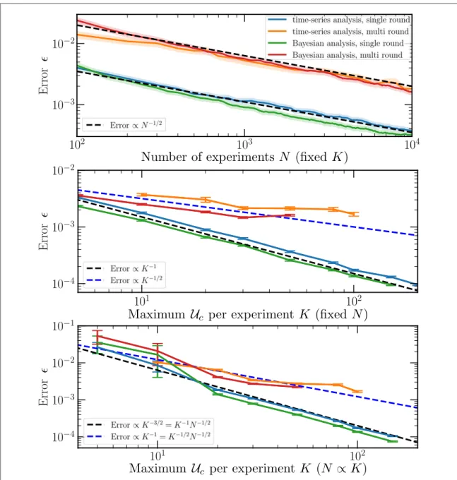
We see that both estimators achieve the previously-derived bounds in3.1(overlayed as dashed lines), and both estimators achieve almost identical convergence rates. The results for the Bayesian estimation match the scaling observed in[10]. Due to the worse scaling inK, the multi-roundk=1 estimation significantly

underperforms single-round phase estimation. This is a key observation of this paper, showing that if the goal is to estimate a phase rather than to project onto an eigenstate, it is preferable to do single-round experiments. 4.2. Example behavior with multiple eigenvalues

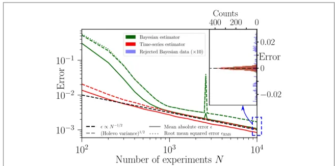
The performance of QPE is dependent on both the estimation technique and the system being estimated. Before studying the system dependence, wefirst demonstrate that our estimators continue to perform at all in the presence of multiple eigenvalues. Infigure4, we demonstrate the convergence of both the Bayesian and time-series estimators in the estimation of a single eigenvaluef0=−0.5 of afixed unitaryU, given a starting state∣Y ñ0 which is a linear combination of 10 eigenstates∣f_jñ. Wefix∣áf₀∣Y ñ =0 ∣2 0.5, and draw other eigenvalues and amplitudes at random from[0,π](making the minimium gapfj−f0equal to 0.5). We perform 2000 QPE

simulations withK=50, and calculate the mean absolute errorò(equation(35), solid), Holevo variance ei 2 1

á ñf -

-∣ ˜ ∣ (dashed), and root mean squared errorrms(dotted), given by 8

Note that this strategy is the opposite of textbook phase estimation in which one necessarily learns the least-significant bit off0firstby

min , 2 Arg e . 35 rms

2 2 i 2

 _≔ á _(∣f-f_{˜ ∣} p-_∣f-f_{˜ ∣)} ñ = á_{∣ (} (f f-˜ )_)∣ ñ _{( )}

We observe that both estimators retain their expected_µN-1 2_{, with one important exception. The Bayesian} estimator occasionally(10% of simulations)estimates multiple eigenvalues nearf0. When this occurs, the

estimations tend to repulse each other, making neither a good estimation of the target. This is easily diagnosable without knowledge of the true value off0by inspecting the gap between estimated eigenvalues. While using this

data to improve estimation is a clear target for future research, for now we have opted to reject simulations where such clustering occurs(in particular, we have rejected data points wheremin( ¯f₀-f¯ )_j <0.05). That this is required is entirely system-dependent: wefind the physical Hamiltonians studied later in this text to not experience this effect. We attribute this difference to the distribution of the amplitudesAj—physical Hamiltonians tend to have a few largeAj, whilst in this simulation theAjwere distributed uniformly.

In the inset tofigure4, we plot a histogram of the estimated eigenphases afterN=104experiments. For the Bayesian estimator, we show both the selected(green)and rejected(blue)eigenphases. We see that regardless of whether rejection is used, the distribution appears symmetric about the target phasef0. This suggests that in the

absence of experimental noise, both estimators are unbiased. Proving this definitively for any class of systems is difficult, but we expect both estimators to be unbiased providedA0?1/K. WhenA0„1/K, one can easily

Figure 3.Estimator performance for single eigenvalues with single and multi-roundk_=1 QPE schemes. Plots show scaling of the mean absolute error(equation(35))with(top)the number of experiments(atfixedK=50), with(middle)Kfor afixed total number of experiments₍N_=106_{), and(bottom)withKwith afixed number(100)of experiments perk=1,K,K(i.e.N=200K). Data is}

averaged over 200–500 QPE simulations, with a new eigenvalue chosen for each simulation. Shaded regions(top)and error bars

construct systems for which no phase estimation can provide an unbiased estimation off0(following the

arguments of section3). We further see that the scaling of the rms erroròrmsand the Holevo variance match the behavior of the mean absolute errorò, implying that our results are not biased by the choice of estimator used. 4.3. Estimator scaling with two eigenvalues

The ability of QPE to resolve separate eigenvalues at smallKcan be tested in a simple scenario of two eigenvalues,

f0andf1. The input to the QPE procedure is then entirely characterized by the overlapA0with the target state

0 fñ

∣ , and the gapd=∣f₀-f₁∣.

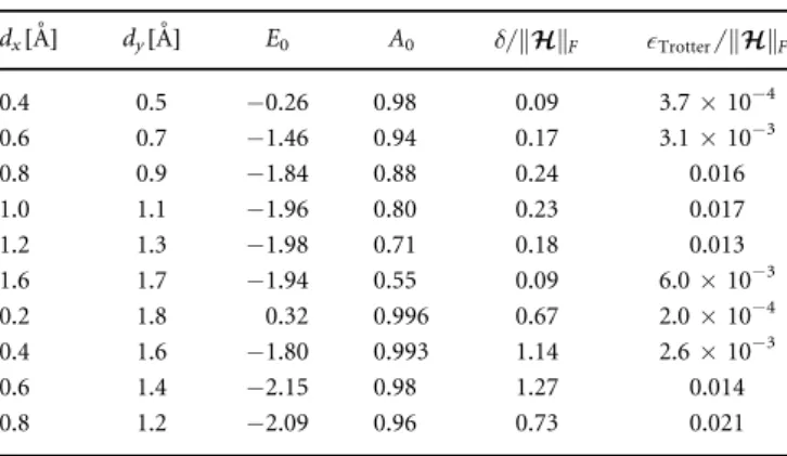
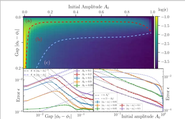
Infigure5, we study the performance of our time-series estimator in estimatingf0afterN=106

experiments withK=50, measured again by the mean errorò(equation(35)). We show a two-dimensional plot

(averaged over 500 simulations at each pointA0,δ)and log–log plots of one-dimensional vertical(lower left)and

horizontal(lower right)cuts through this surface. Due to computational costs, we are unable to perform this analysis with the Bayesian estimator, or for the multi-round scenario. We expect the Bayesian estimator to have similar performance to the time-series estimator(given their close comparison in sections4.1and4.2). We also expect the error in multi-round QPE to follow similar scaling laws inA0andδas single-round QPE(i.e.

multi-round QPE should be suboptimal only in its scaling inK).

The ability of our estimator to estimatef0in the presence of two eigenvalues can be split into three regions

(marked as(a),(b),(c)on the surface plot). In region(a), we have performed insufficient sampling to resolve the eigenvaluesf0andf1, and QPE instead estimates the weighted average phaseA0f0+A1 1f. The error in the estimation off0then scales by how far it is from the average, and how well the average is resolved

A K N

1 0 1 1 2. 36

µ₍ - ₎d - - _{( )}

In region(b), we begin to separatef0, from the unwanted frequencyf1, and our convergence halts

A₀1 2. 37

µ - d- _{( )}

In region(c), the gap is sufficiently well resolved and our estimation returns to scaling well withNandK

A01K N1 1 2. 38

µ - - - _{( )}

The scaling laws in all three regions can be observed in the various cuts in the lower plots offigure5. We note that the transition between the three regions is not sharp(boundaries estimated by hand), and isKandN-dependent. 4.4. Many eigenvalues

To show that our observed scaling is applicable beyond the toy 2-eigenvalue system, we now shift to studying systems of random eigenvalues withNeig>1. In keeping with our insight from the previous section, infigure6

Figure 4.Scaling of error for time-series₍dark green₎and Bayesian₍red₎estimators with the number of experiments performed for a single shot of a unitary with randomly drawn eigenphases(parameters given in text). Three error metrics are used as marked

(described in text—note that the mean squared error and Holevo variance completely overlap for the time-series estimator). Data is averaged over 2000 simulations. The peak nearN=3000 comes from deviation in a single simulation and is not of particular interest. With this exception, error bars are approximately equal to width of the lines used.(Inset)histogram of the estimated phases after

wefixf0=0, and study the erroròas a function of the gap

min . 39

j 1 j 0

d= f -f

> (∣ ∣) ( )

WefixA0=0.5, and draw the other parameters for the system from a uniform distribution:fj∼[δ,π],Aj∼[0, 0.5](fixingåN_j=eig1Aj = -1 A0). We plot both the average errorò(line)and the upper 47.5% confidence interval

Figure 5.Performance of the time-series estimator in the presence of two eigenvalues.₍Top₎surface plot of the error afterN_=106

experiments forK=50, as a function of the overlapA0with the target state∣f0ñ, and the gap∣f0-f1∣. Plot is divided by hand into three labeled regions where different scaling laws are observed. Each point is averaged over 500 QPE simulations.₍bottom₎log_–log plots of vertical(bottom left)and horizontal(bottom right)cuts through the surface, at the labeled positions. Dashed lines in both plots arefits(by eye)to the observed scaling laws. Each point is averaged over 2000 QPE simulations, and error bars give 95% confidence intervals.

Figure 6.Performance of the time-series estimator in the presence of multiple eigenvalues. Error bars show 95% confidence intervals

[ò,ò+2σò](shaded region)for various choices ofNeig. We observe that increasing the number of spurious

eigenvalues does not critically affect the error in estimation; indeed the error generally decreases as a function of the number of eigenvalues. This makes sense; at largeNeigthe majority of eigenvalues sit in region(c)offigure5, and we do not expect these to combine to distort the estimation. Then, the nearest eigenvalueminj¹0fjhas on

average an overlapAj µ1 Neig, and its average contribution to the error in estimatingf0(inasmuch as this can

be split into individual contributions)scales accordingly. We further note that the worst-case error remains that of two eigenvalues at the crossover between regions(a)and(b). In appendixDwe study the effect of confining the spurious eigenvalues to a region[d f, _max]. We observe that when most eigenvalues are confined to regions

(a)and(b), the scaling laws observed in the previous section break down, however the worst-case behavior remains that of a single spurious eigenvalue. This implies that sufficiently longKis not a requirement for QPE, even in the presence of large systems or small gapsδ; it can be substituted by sufficient repetition of experiments. However, we do require that the ground state is guaranteed to have sufficient overlap with the starting

state—A0>1/K(as argued in section3). As QPE performance scales better withKthan it does withN, a

quantum computer with coherence time2Tis still preferable to two quantum computers with coherence timeT

(assuming no coherent link between the two).

5. The effect of experimental noise

Experimental noise currently poses the largest impediment to useful computation on current quantum devices. As we suggested before, experimental noise limitsKso that forKKerrthe circuit is unlikely to produce reliable results. However, noise on quantum devices comes in variousflavors, which can have different

corrupting effects on the computation. Some of these corrupting effects(in particular, systematic errors)may be compensated for with good knowledge of the noise model. For example, if we knew that our system applied

U₌e-i(t+)_{instead ofU=e}-it_{, one could divide}

0

f˜ _{by(t+ò)/tto precisely cancel out this effect. In this}

study we have limited ourselves to studying and attempting to correct two types of noise: depolarizing noise, and circuit-level simulations of superconducting qubits. Given the different effects observed, extending our results to other noise channels is a clear direction for future research. In this section we do not study multi-round QPE, so each experiment consists of a single round. A clear advantage of the single-round method is that the only

relevanteffect of any noise in a single-round experiment is to change the outcome of the ancilla qubit,

independent of the number of system qubitsnsys. 5.1. Depolarizing noise

A very simple noise model is that of depolarizing noise, where the outcome of each experiment is either correct with some probabilitypor gives a completely random bit with probability1-p. We expect this probabilitypto depend on the circuit time and thus the choice ofk…0, i.e.

p=p k_{( )}=e-k Kerr. ₍40₎

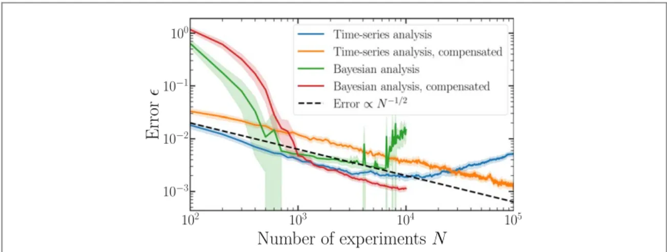
Figure 7.Convergence of Bayesian and time-series estimators in the presence of depolarizing noise and multiple eigenvalues, both with and without noise compensation techniques(described in text). Fixed parameters for all plots are given in text. Shaded regions denote a 95% confidence interval(data estimated over 200 QPE simulations). The black dashed line shows theN−1/2_convergence

We can simulate this noise by directly applying it to the calculated probabilitiesPk,b( ∣ )mf for a single round

P m P m p k 1 p k

2 . 41

k, f  k, f +

-b( ∣ ) b( ∣ ) ( ) ( ) ( )

Infigure7, we plot the convergence of the time-series(blue)and Bayesian(green)estimators as used in the previous section as a function of the number of experiments, withfixedK=50=Kerr 2fixed,A0=0.5,

Neig=10andδ=0.5. We see that both estimators obeyN−1/2scaling for some portion of the experiment, however this convergence is unstable, and stops beyond some critical point.

Both the Bayesian and time-series estimator can be adapted rather easily to compensate for this

depolarizing channel. To adapt the time-series analysis, we note that the effect of depolarizing noise is to send

g k( )g k p k( ) ( )whenk>0, via equation(23)and equation(41). Our time-series analysis was previously performed over the rangek= -K,¼,K(gettingg(-k)=g k*( )for free), and over this range

g k( )g k p k( ) (∣ ∣). (42)

g(k)is no longer a sum of exponential functions over our interval[-K K, ], as it is not differentiable atk=0, which is the reason for the failure of our time-series analysis. However, over the interval[0,K]this is not an issue, and the time-series analysis may still be performed. If we construct a shift operatorTusingg(k)from

k=0,K,K, this operator will have eigenvalueseifj-1 Kerr_{. This then implies that the translation operatorTcan}

be calculated usingg(k)withk>0, and the complex argument of the eigenvalues ofTgive the correct phasesfj. We see that this is indeed the case infigure7(orange line). Halving the range ofg(k)that we use to estimatef0

decreases the estimator performance by a constant factor, but this can be compensated for by increasingN. Adapting the Bayesian estimator requires simply that we use the correct conditional probability, equation(41). This in turn requires that we either have prior knowledge of the error rateKerr, or estimate it

alongside the phasesfj. For simplicity, we opt to choose the former. In an experimentKerrcan be estimated via

standard QCVV techniques, and we do not observe significant changes in estimator performance when it is detuned. Our Fourier representation of the probability distribution off0can be easily adjusted to this change.

The results obtained using this compensation are shown infigure7: we observe that the data follows aN−1/2

scaling again.

5.2. Realistic circuit-level noise

Errors in real quantum computers occur at a circuit-level, where individual gates or qubits get corrupted via various error channels. To make connection to current experiments, we investigate our estimation performance on an error model of superconducting qubits. Full simulation details can be found in appendixE. Our error model is primarily dominated byT1andT2decoherence, incoherent two-qubitflux noise, and dephasing during

single-qubit gates. We treat the decoherence timeTerr=T1=T2as a free scale parameter to adjust throughout

our simulations, whilst keeping all other error parameters tied to this single scale parameter for simplicity. In order to apply circuit-level noise we must run quantum circuit simulations, for which we use the quantumsim density matrix simulatorfirst introduced in[37]. We then choose to simulate estimating the ground state energy of four hydrogen atoms in varying rectangular geometries, with Hamiltoniantaken in the STO-3G basis calculated via psi4[38], requiringnsys =8qubits. We make this estimation via a lowest-order Suzuki-Trotter approximation[39]to the time-evolution operatore-it_{. To prevent energy eigenvalues wrapping around the}

circle wefixt=1 Trace_[ † _{] (}2nsys₎9_{. The resultant 9-qubit circuit is made using the OpenFermion}

package[9].

In lieu of any circuit optimizations(e.g.[23,40]), the resulting circuit has a temporal length per unitary of

TU=42 sm (with single-(two-)qubit gate times 20 ns(40 ns)). This makes the circuit unrealistic to operate at current decoherence times for superconducting circuits, and we focus on decoherence times 1−2 orders of magnitude above what is currently feasible, i.e.Terr=5−50 ms. However one may anticipate that the ratio

TU/Terrcan be enlarged by circuit optimization or qubit improvement. Naturally, choosing a smaller system,

less than 8 qubits, or using error mitigation techniques could also be useful.

We observe realistic noise to have a somewhat different effect on both estimators than a depolarizing channel. Compared to the depolarizing noise, the noise may(1)be biased towards 0 or 1 and/or(2)its dependence onkmay not have the form of equation(40).

Infigure8, we plot the performance of both estimators at four different noise levels(and a noiseless simulation to compare), in the absence of any attempts to compensate for the noise. Unlike for the depolarizing channel, where aN−1/2convergence was observed for some time before the estimator became unstable, here we 9

see both instabilities and a loss of theN−1/2decay to begin with. Despite this, we note that reasonable convergence(to within 1%−2%)is achieved, even at relatively low coherence times such asKerr=10.

Regardless, the lack of eventual convergence to zero error is worrying, and we now shift to investigating how well it can be improved for either estimator.

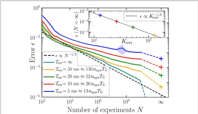
Adjusting the time-series estimator to use onlyg(k)for positivekgives approximately 1−2 orders of magnitude improvement. Infigure9, we plot the estimator convergence with this method. We observe that the estimator is no longer unstable, but theN−1/2convergence is never properly regained. We may study this convergence in greater deal for this estimator, as we may extractg(k)directly from our density-matrix simulations, and thus investigate the estimator performance in the absence of sampling noise(crosses on screen). We note that similar extrapolations in the absence of noise, or in the presence of depolarizing noise

Figure 8.Performance of Bayesian(solid)and time-series(dashed)estimators in the presence of realistic noise without any compensation techniques. Shaded regions denote 95% confidence intervals(averaged over 100–500 QPE simulations). The time-series analysis requiresN>2Kexperiments in order to produce an estimate, and so its performance is not plotted forN<100.

Figure 9.Performance of time-series estimator with compensation techniques(described in text). Shaded regions denote 95% confidence intervals(averaged over 200 QPE simulations). Final crosses show the performance in the absence of any sampling noise

(teal cross is at approximately 10−10_{), i.e. in the limitN ¥;dashed lines are present to demonstrate this limit.(Inset)plot of error}

(when compensated)give an error rate of around 10−10, which we associate tofixed-point error in the solution to the least squares problem(this is also observed in the curve without noise infigure9). Plotting this error as a function ofKerrshows a power-law decay -µKerr-aµTerr-awitha=1.9»2. We do not have a good understanding of the source of the obtained power law.

The same compensation techniques that restored the performance of the Bayesian estimator in the presence of depolarizing noise do not work nearly as well for realistic noise. Most likely this is due to the fact that the actual noise is not captured by ak-dependent depolarizing probability. Infigure10we plot the results of using a Bayesian estimator when attempting to compensate for circuit-level noise by approximating it as a depolarizing channel with a decay rate(equation(40))ofKerr=Terr T nU sys. This can be compared with the results offigure8 where this compensation is not attempted. We observe a factor 2 improvement at lowTerr, however theN−1/2

scaling is not regained, and indeed the estimator performance appears to saturate at roughly this point. Furthermore, atTerr=50 ms, the compensation techniques do not improve the estimator, and indeed appear

to make it more unstable.

To investigate this further, infigure10(inset)we plot a Bayes factor analysis of the Bayesian estimators with and without compensation techniques. The Bayes factor analysis is obtained by calculating the Bayes factors

F P m M

P m M , 43

n n

n

expt



= ( ∣ )

( ∣ ) ( )

Figure 10.Performance of single-round Bayesian QPE with four sets of realistic noise using a compensation technique described in the text. Shaded regions are 95% confidence intervals over 200–500 QPE simulations.(Inset)a Bayes factor analysis for the data below. Line color and style matches the legend of the mainfigure.

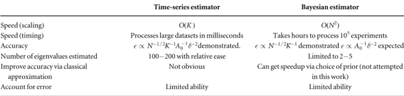
Table 1.Table comparing metrics of interest between the two studied estimators. All metrics are implementation-specific, and may be improvable.

Time-series estimator Bayesian estimator

Speed₍scaling₎ O₍K₎ O₍N2₎

Speed(timing) Processes large datasets in milliseconds Takes hours to process 105experiments

Accuracy N 1 2K A1

01 2

µ - - - -d _{demonstrated. µN}-1 2_K-1_{demonstrated A} 01 2

µ - -d _expected.

Number of eigenvalues estimated 100₋200 with relative ease Limited to 2₋5 Improve accuracy via classical

approximation

Not obvious Can get speedup via choice of prior(not attempted in this work)