PARAMETER OPTIMIZATION ON THE CONVERGENCE SURFACE OF PATH SIMULATIONS
SRINIVAS NIRANJ CHANDRASEKARAN
A dissertation submitted to the faculty at the University of North Carolina at Chapel Hill in partial fulfillment of the requirements for the degree of Doctor of Philosophy in the Department of
Biochemistry and Biophysics in the School of Medicine
Chapel Hill 2016
Approved by: Sharon L. Campbell Charles W. Carter Jr. Nikolay V. Dokholyan Jan Hermans
ii © 2016
iii ABSTRACT
Srinivas Niranj Chandrasekaran: Parameter optimization on the convergence surface of PATH simulations
(Under the supervision of Charles W. Carter Jr.)
all-iv
v
vi
ACKNOWLEGDEMENTS
Firstly, I would like to thank my mentor, Dr. Charles Carter, for encouraging me to pursue a challenging project and helping me at each step to overcome many hurdles. I would like to thank him for not losing patience with me, the tens of times I came up with a new solution to the parameter optimization problems, raising everyone’s hopes only to came back the very
next morning to tell him that method worked only for special cases. His perseverance and his enthusiasm for the project motivated me during times when the project was stuck and progress was hard to come by. As a mentor, he also provided me with many anecdotal advices, which have been invaluable in shaping my career.
I would also like to thank Dr. Jan Hermans for helping me think about PATH in a new way which was crucial in finding a solution to the optimization problem and in the development of the current version of PATH. He graciously spent several afternoons with me listening to and critiquing my ideas which were important for my development as a scientist.
I would like to thank my committee members Drs. Nikolay V. Dokholyan, Sharon Campbell and Qi Zhang. I collaborated with Dr. Dokholyan for validating the PATH results, during which I had the opportunity of interact with him several times which were instrumental in figuring out the correct approach to test PATH. Dr. Campbell guided me when I was not able to find a suitable lab during my lab rotation and helped me join Dr. Carter’s lab. With Dr. Zhang I
have had several fruitful discussions during my committee meetings for which I am thankful.
vii
Finally, I would like to thank my family. My parents have always been supportive and have stood by my side in every academic decision that I have made. They have always
encouraged me to pursue by goals and choose the career that I was interested in. Last of all, I would to thank my wife, Priya, who has made the pursuit of science an enjoyable experience. It is great to be able to discuss my work with her, as she is a fellow scientist, and she has
viii PREFACE
Part of the work described here was published in the journal Structural Dynamics:
ix
TABLE OF CONTENTS
LIST OF TABLES ... xii
LIST OF FIGURES ...xiii
LIST OF ABBREVIATIONS ... xiv
CHAPTER 1: INTRODUCTION ... 1
1.1 Conformational transition states impose multistate behavior in proteins ... 2
1.2 Identification of conformational transition states by computational methods ... 2
1.3 PATH rapidly computes the most likely path and transition state ... 6
1.4 Minimum action pathways depend on several input parameters ... 7
CHAPTER 2: THEORY OF PATH ... 10
2.1 Protein conformational change as a stochastic process ... 10
2.2 Equation of motion of the most probable path... 12
2.2.1 Classical Action ... 12
2.2.2 Onsager-Machlup equations of motion ... 14
2.3 Using PATH for a two state system ... 15
2.3.1 1D diatomic system ... 15
2.3.2 3D N atom system ... 19
CHAPTER 3: MODIFICATION OF PATH ... 25
3.1 Optimization of 𝒕𝒇 ... 25
x
3.1.2 Intermediate values of 𝑡𝑓 ... 28
3.1.3 Large values of 𝑡𝑓 ... 30
CHAPTER 4: VALIDATION AND RESULT FROM PATH SIMULATIONS ... 40
4.1 PATH, ANMPathway and the String trajectories agree most closely with each other at their transition states ... 40
4.2 Discrete molecular dynamics replica exchange simulations verify that transition states identified by path are close to saddle points in the free energy surface connecting initial and final states ... 42
4.3 Transition states identified by PATH display comparable rate-limiting structures in three different systems ... 45
CHAPTER 5: MATERIALS AND METHODS ... 47
5.1 Structures ... 47
5.2 PATH simulations ... 47
5.3 ANMPathway simulations ... 48
5.4 DMD simulations... 48
5.5 Fitting the Free energy surfaces ... 49
5.6 Design of computational mutants ... 49
CHAPTER 6: CONCLUSION AND FUTURE DIRECTIONS ... 51
6.1 Output parameters from PATH can be used to model experimentally determined kinetic 𝚫𝚫𝑮 values for TrpRS mutants ... 52
6.2 Modifying the PATH Hessian ... 54
6.3 Including potential to constrain the torsional angles ... 58
6.4 Conclusion ... 60
xi
xii
LIST OF TABLES
Table 1...54
xiii
LIST OF FIGURES
Figure 1. The double well.………...7
Figure 2. The convergence surface………...9
Figure 3. Toy model………...12
Figure 4. Two states of the 1D system………...15
Figure 5. 𝑄1 vs. 𝑡 at small 𝑡𝑓………...28
Figure 6. 𝑄1 vs. 𝑡 at intermediate values of 𝑡𝑓………...29
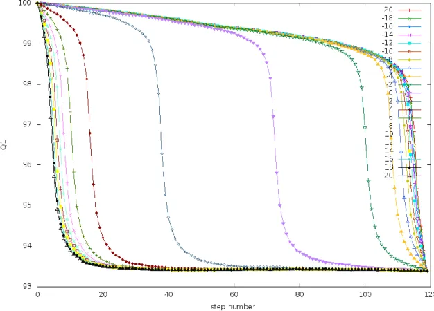
Figure 7. 𝑄1 vs. 𝑡 at large values of 𝑡𝑓...30
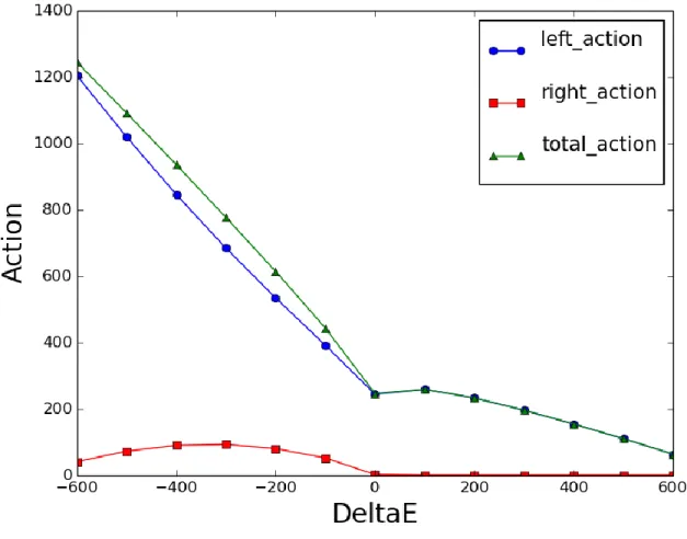
Figure 8. Action vs DE with the old equation for right action...32
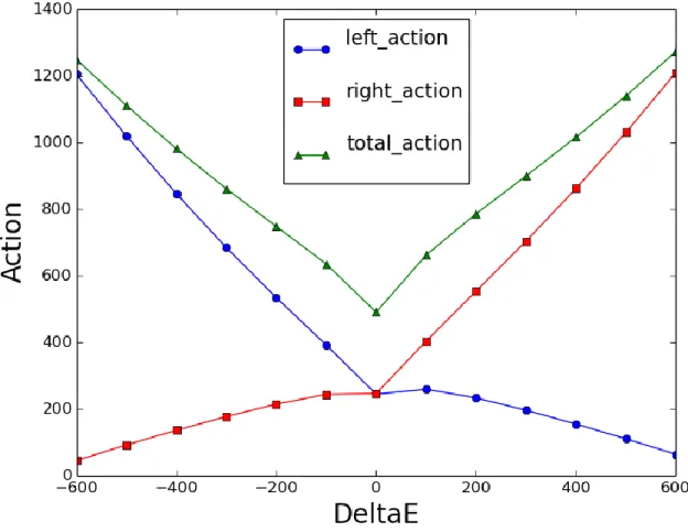
Figure 9. Action vs DE with the new equation for right action...35
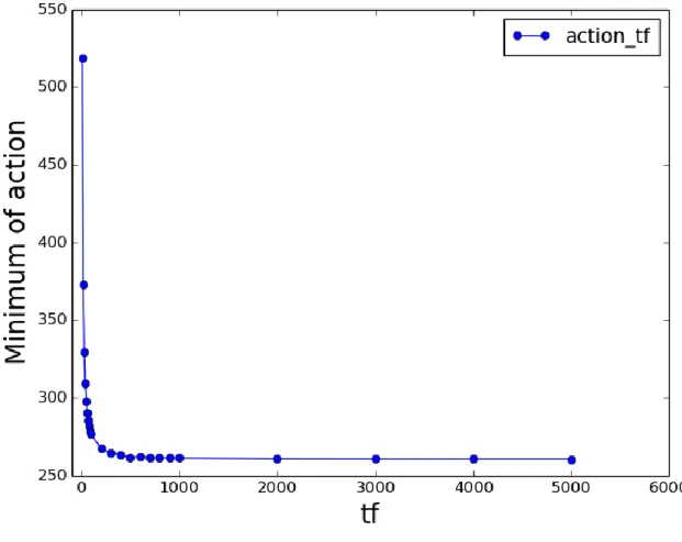
Figure 10. Minimum of action vs. 𝑡𝑓...36
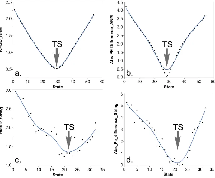
Figure 11. PATH vs. ANMPathway and String...41
Figure 12. Free energy surface from Replica exchange DMD...44
Figure 13. Transition states of three different systems...46
Figure 14. Prediction of experimentally determined kinetic free energy using PATH...53
xiv
LIST OF ABBREVIATIONS
ANM Anisotropic Network Model
CHARMM Chemistry at HARvard Molecular Mechanics
DMD Discrete Molecular Dynamics
MD Molecular Dynamics
NMA Normal Mode Analysis
NMR Nuclear Magnetic Resonance Spectroscopy
RMSD Root Mean Squared Deviation
1
CHAPTER 1: INTRODUCTION
Enzyme catalyzed reactions form an integral part of biology and are fundamentally important for replication of genetic material and for the survival of life. Hence enzyme catalyzed reactions have been studied in great detail, starting from simple catalysis of oligosaccharides by lysozyme (Chipman 1971) to complex reactions like mRNA translation by Ribosomes (Fluitt et al. 2007). In general, enzyme catalyzed reactions often take place in two steps, the fast
chemical reaction step and the slower, rate-limiting protein conformational change step (Watt et al. 2007). The former is well understood for many enzyme catalyzed reactions because the transition states of the reaction are well characterized. One of the common ways to study these transition states is to arrest the reaction at the transition state using a transition state analog (Secemski et al. 1972). This is possible because the structure of the chemical species at the transition state is well known. Also, the chemical reaction is a localized phenomenon, that is, the parts of the protein that are involved in the chemical reaction are in and around the reactants in the binding pocket
2
1.1 Conformational transition states impose multistate behavior in proteins Conformational transition states are the most energetic structures along the
conformational change pathways of proteins. Understanding the nature of these transition states is important as they hold information regarding what causes proteins to exist in multiple states (Kapustina et al. 2007). The multistate behavior of proteins is fundamental to life as it provides a way to generate states with a free energy differential and the transition between such states happens as a response to stimulus. Such conformational transitions can act as molecular timers to help regulate amplitude and duration of cellular processes (Nicholson & Lu 2007),
significantly enhancing function by creating the capacity for a protein to transmit time and ligand-dependent information and/or mechanical motion necessary for signaling and other free-energy transduction processes. Structures of conformational transition states should therefore reveal valuable information about the energy barriers that separate one equilibrium structure from another.
1.2 Identification of conformational transition states by computational methods
Traditional experimental methods that are used for determination of macromolecular structure, like NMR and X-ray crystallography, cannot be used to identify the structures of conformational transition states, due to their fleeting existence. Hence computational methods have to be used to identify and characterize conformational transition states.
Molecular Dynamics (MD) simulations are the most commonly used computational methods to study the time evolution of macromolecular structures. There are several well-established force fields and algorithms, such as, GROMACS (Lindahl et al. 2001; Hess et al. 2008), CHARMM (Brooks et al. 1983; Brooks et al. 2009), AMBER (Cornell et al. 1995) and NAMD (Phillips et al. 2005), that are the most widely used tools for performing
3
studying folding pathways of smaller proteins (Shaw et al. 2010). But to identify
conformational transition states MD simulations are inefficient tools, because, the protein conformational changes occur on the timescale of milliseconds and it is difficult to simulate large proteins for that time. Also as conformational changes are very rare compared to the rest of the time the protein spends at the equilibrium state identifying these conformational transition states in a statistically significant ensemble would require several transitions between the equilibrium states, which is really difficult to simulate.
In spite of these problems, MD simulations can still provide useful information about protein conformational changes and transition states when coupled with sampling
algorithms. One such popular algorithm is Steered Molecular Dynamics (Baker et al. 2013) where a force is applied to a part of a protein so that the transition from one state to another is induced. This speeds up the simulation and the different conformations can be sampled more rapidly. Another such algorithm is the Umbrella Sampling method (Torrie & Valleau 1977) where the energy barrier separating the two conformations is flattened such that the two states are sampled. Another recent, but popular, method is the replica exchange algorithm (Sugita & Okamoto 1999) which provides comprehensive mapping of the
conformational free energy landscape. The replica exchange algorithm efficiently searches the configuration space of proteins by overcoming the sampling problem that affects single temperature simulations, which is that, at low temperatures the structures do not have enough energy to overcome conformational barriers and at high temperatures, the structures are unfolded and are far from the equilibrium states. In replica exchange simulations, multiple replicas of the starting structure are simulated at different temperatures and at defined time intervals, structures at different temperatures are
exchanged. By doing this, replica exchange simulations allow systems to explore structures at different temperatures, thus sampling the conformational landscape, quickly and
4
There are other molecular dynamics simulation algorithms that increase the speed of simulations by different kinds of simplification like Discrete Molecular Dynamics (DMD) (Ding et al. 2008; Dokholyan et al. 1998; Shirvanyants et al. 2012). DMD uses a step-wise potential energy function instead of the smooth functions that other force fields use, which decreases the frequency at which the force has to be computed. This also means that the forces are computed not at regular intervals of time but is event based, that is, the force is computed when an event occurs. Hence DMD speeds up molecular dynamics simulations and with the help of a sampling algorithm (Williams II et al. 2015), can rapidly generate conformational landscapes.
Even though there are good sampling algorithms and quick MD simulations
techniques, they are still time and resource intensive. Some dedicated algorithms (Fujisaki et al. 2010) sample transition paths in the neighborhood of the most probable pathways between two equilibrium states, thereby not requiring massive computational resources. Once such algorithm is the String method (E et al. 2002b; Ovchinnikov et al. 2011) which furnishes an analytical algorithm for mapping the most probable path through
conformational free energy landscapes using intervals between nodes defined in terms of collective variables along the path. It describes the transition pathway as the curve that connects successive metastable states so as to maintain a tangential projection of the curvature of the collective variables with respect to Cartesian space onto the free energy surface defined by the collective variables. Using collective variables reduces the number of degrees of freedom over which MD simulations are required. The progress between
5
considered to be the gold standard in the field. In spite of the success of the string method, it is nevertheless resource intensive.
Many functional conformational changes are distinct from protein folding reactions in that they entail primarily large amplitude motions that are independent of individual covalent bond vibration. Often, these conformational changes are rigid-body motions that can be replicated by the superposition of a few large amplitude normal modes. Numerous algorithms have been introduced to exploit Elastic Network Models (ENM) (Bahar et al. 1997) in the computation of conformational change trajectories like Plastic Network Model (Maragakis & Karplus 2005) and adaptive Anisotropic Network Model (aANM) (Yang et al. 2009). In PNM, the conformational change trajectory is computed by minimizing the path integral of a free energy functional corresponding to the action or “resistance” along the
path. This computed trajectory is a minimum energy path and is a differentiable curve through the centers of a smooth tube in pathspace containing the most probable paths (Durr & Bach 1978; Pinski & Stuart 2010). In aANM, the trajectory is calculated by an iterative method in which the intermediate state between the two equilibrium states are identified along the distance vector connecting the initial and the final states. Another related algorithm is ANMPathway (Das et al. 2014) which uses an Anisotropic Network Model (ANM) (Atilgan et al. 2001) to describe the potential energy wells of the two
equilibrium states. In this method, the two structures are linearly extrapolated such that the energy of the two intermediates states, relative to the end states are equal. These two intermediate states now define a cusp hyperspace on which the lowest energy structure is identified by energy minimization, which is the transition state. Then by steepest descent energy minimization the trajectory from the transition state, back to the equilibrium states is computed.
6
transition state structures. It can be argued that in many ways transition-state structures, not the exact path, may be what are most important about conformational transitions. Hence my project was on the investigation of the possibility that the simplified potentials may furnish a sufficient basis set to identify valid transition state structures for large domain motions. Thus, whereas most treatments focus on the trajectories; I focused on the
transition states themselves because they contain information about the barriers that impose multi-state behavior on proteins.
1.3 PATH rapidly computes the most likely path and transition state
PATH (formerly MinActionPath (Franklin et al. 2007)) is an algorithm that rapidly computes conformational transition states and the associated trajectories by minimizing the Onsager-Machlup (OM) functional (Onsager & Machlup 1953). The probability of finding a stochastic system at a given position and time is given by the Fokker-Planck equation.The OM functional is derived from the solution to the Fokker-Planck equation (Onsager & Machlup 1953) such that its minimization by a variational computation, implemented using the Euler-Lagrange equations, furnishes equations of motion describing the most probable path.
PATH defines the structures of equilibrium states using a linearized ANM potential. This approximation of the complex potential energy landscape works because most protein conformational changes are small displacements from the equilibrium states. PATH uses either all atom or more limited ANM models to identify the transition state. Then, it
computes paths to and from that transition state using the OM equations of motion. PATH is an efficient algorithm for identifying the transition state and also the conformational change pathway that passes through it.
7
1.4 Minimum action pathways depend on several input parameters
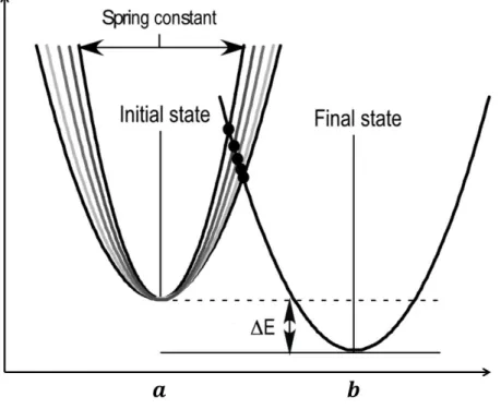
PATH models the two equilibrium structures, between which the path has to be computed, as harmonic potential wells and the point of intersection of the two wells as the transition state. The shapes of the harmonic wells are defined by force constants 𝑘𝑙 and 𝑘𝑟 for
the left and the right potential wells respectively (Fig. 1)
Figure 1. The double well: The two states of the protein between which the transitions are
studied, can be approximated by the double well system. 𝑎 and 𝑏 are the two equilibrium states which are
separated by an energy barrier. Δ𝐸 is the energy difference between the two minima. The width of the
well is given by the value of the force (spring) constants, the narrower the well, the greater the value of
the force constants.
The two structures are input crystal structures, 𝑎 and 𝑏, and the force constants are calculated from the second derivative of the potential, called the Hessian Matrix. At the point of intersection of the two wells, which is the transition state 𝑥̅, the two wells have the same energy 𝑈‡ . If the total time taken to make the full transition is considered to be 𝑡
8
reach the transition state from the initial state, 𝑡̅, is a fraction of the total time and it uniquely identifies each minimum action path at that 𝑡𝑓.
From Fig. 1, it can be seen that if either force constant, 𝑘𝑙 or 𝑘𝑟, the relative energy
difference between the two wells (Δ𝐸), or 𝑡𝑓 are changed, then the minimum action path that the
system will take would be different. This means that for different values of Δ𝐸 and 𝑡𝑓 and as
noted previously (Pinski & Stuart 2010) there are different minimum action paths between the given equilibrium states, each defined by a different 𝑡̅. As previously mentioned, since 𝑡̅ uniquely identifies each path, when plotted against different values of Δ𝐸 and 𝑡𝑓 it gives rise to the
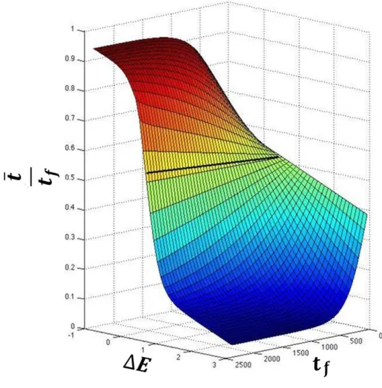
surface that I call the convergence surface (Fig. 2).
This surface represents all the possible minimum action trajectories between a given pair of structures and it is different for different pairs of structures. This surface also shows the bi-sigmoidal behavior of 𝑡̅ with respect to both Δ𝐸 and 𝑡𝑓. This surface also means that multiple,
locally minimum action paths are possible for the same pair of structures. Appropriate values of both Δ𝐸 and 𝑡𝑓 must therefore be chosen to identify a single minimum action path and transition
state that is closest to what is observed in nature.
9
Figure 2. The convergence surface: From Fig. 1, it can be seen that the path must depend on
both Δ𝐸 and 𝑡𝑓. Since 𝑡̅, at each value of 𝑡𝑓, uniquely identifies a path as a function of Δ𝐸, it gives rise to
the convergence surface shown in this figure.The surface was obtained from simulations of the catalytic
step of Tryptophanyl-tRNA synthetase and fitted to an empirical equation (𝑅2= 0.99). The surface shows
a sigmoidal dependence of 𝑡̅ on both Δ𝐸 and 𝑡𝑓. Since only positive values of 𝑡𝑓 are used in the
simulations, only the lower half of the sigmoid is seen along the 𝑡𝑓 axis and it can be fitted approximately
10
CHAPTER 2: THEORY OF PATH
2.1 Protein conformational change as a stochastic process
Protein conformational changes are diffusive processes, which can be modeled using an overdamped Langevin equation. In the overdamped regime there is no acceleration which means that the energy gained by interaction with the random force, is also lost quickly due to friction.
In one dimension, the Langevin equation can be written as
𝑚𝛾𝑥̇ = −d𝑉
𝑑𝑥+ √2𝑚𝛾𝑘𝐵𝑇𝜉 (1)
where, 𝛾 is the diffusion coefficient, −𝑑𝑉
𝑑𝑥 is the force that causes the drift and 𝜉 is a
delta-correlated Gaussian random force, with zero mean. That is,
〈𝜉(𝑡)〉 = 0 (2)
〈𝜉(𝑡)𝜉(𝑡′)〉 = 𝛿(𝑡 − 𝑡′) (3)
In the case of proteins, the drift force arises from the interatomic interactions which are modeled in PATH as linearized Anisotropic Network Model (ANM). The potential in ANM is written as
𝑉 =𝑘
2(𝑥 − 𝑎)
2 (4)
11
𝑚𝛾𝑥̇ = −𝑘(𝑥 − 𝑎) + √2𝑚𝛾𝑘𝐵𝑇𝜉 (5)
Because of the stochastic nature of the Langevin equation, only the probability of the states that the protein could be in, can be computed, which is in contrast to the ballistic
equations that gives deterministic paths. The probability of these states can be calculated using an alternate form of the Langevin equation called the Fokker-Planck equation.
𝜕𝑝(𝑥, 𝑡)
𝜕𝑡 =
𝜕
𝜕𝑥(−𝑘(𝑥 − 𝑎)𝑝(𝑥, 𝑡)) −
1 2
𝜕2
𝜕𝑥(
2𝑘𝐵 𝑇
𝑚𝛾 𝑝(𝑥, 𝑡))
Then the probability of the protein to reach state 𝑥2 at time 𝑡2 given that that the system
was at state 𝑥1 at time 𝑡1 can be written as
𝑝(𝑥2, 𝑡2|𝑥1, 𝑡1) = 𝑒
−4𝑘𝑘
𝐵𝑇((𝑥1−𝑎)−(𝑥2−𝑎)𝑒 𝑘Δ𝑡 𝑚𝛾)
2
(−1+coth(𝑘Δ𝑡𝑚𝛾) )
(4𝜋𝑘1
𝐵𝑇(𝑘(1 + coth (
𝑘𝛥𝑡 𝑚𝛾 )))
−12
(6)
where, 𝑘𝐵 is the Boltzmann constant, and 𝑇 is the temperature. This is a solution to the
Fokker-Planck equation.
If the total path is a succession of such states, then the joint probability can be calculated as the product of the probabilities of the individual segments. By this method, the probability of each path that goes from one state of the protein to another can be calculated. Since in the case of PATH, only the most probable pathway is of interest, it can be calculated by minimizing the exponent of (6). To do this Onsager and Machlup came up an ingenious method (Onsager & Machlup 1953), where they were able to derive the equation of motion for the most probable path by writing (6) as
𝑝 ∝ 𝑒−
𝑆𝑂𝑀
12
where, 𝑆𝑂𝑀 is an integral called the Onsager-Machlup action functional and it is of the
form
𝑆𝑂𝑀=
1
2𝛾∫ (𝑚𝛾𝑥̇ + 𝑘(𝑥 − 𝑎))
2 𝑑𝑡 𝑡
0
(8)
2.2 Equation of motion of the most probable path
To understand the derivation of the resulting equation of motion for the most probable path from Onsager-Machlup action, it is a useful exercise to compare and calculate the ballistic equations of motion using classical action.
2.2.1 Classical Action
Figure 3. Toy model: The two atoms of a diatomic system interact with each other and this
interaction is modeled as a one-dimensional spring that follows Hook’s law, 𝐹 = −𝑘𝑥, where 𝑘 is the force
constant and 𝑥 is the displacement from the mean position.
Consider a 1D diatomic system (Fig. 3) following Newtonian dynamics in a single potential well. Let the interaction between the two atoms be modeled by a 1D Hookean spring. On the basis of the principle of least action, the equation of motion can be derived by identifying the path that minimizes action. Classical action of a path is defined as the sum over the
Lagrangian at every time instant. It has the mathematical form
𝑆𝑐𝑙 = ∫ 𝐿. 𝑑𝑡 𝑡
0
(9)
13
𝑆𝑐𝑙= ∫ (𝑇 − 𝑉)𝑑𝑡
𝑡
0
(10)
Hence to compute the action of any path and to identify the most probable path, it is required to know the kinetic and potential energies of the system.
Since the potential energy is described by a Hookean spring, it is written as equation (4)
𝑉 =𝑘
2(𝑥 − 𝑎)
2
As the kinetic energy is written as 𝑇 =1 2𝑚𝑥̇
2, the Lagrangian can be written as
𝐿 = 𝑇 − 𝑉 =1
2(𝑚𝑥̇
2− 𝑘(𝑥 − 𝑎)2) (11)
Using (11), (10) can be written as
𝑆𝑐𝑙 = ∫ 1 2(𝑚𝑥̇
2− 𝑘(𝑥 − 𝑎)2)𝑑𝑡 𝑡
0
(12)
Equation (12) computes the action of any given path but the path of minimum action can be identified by calculating the extremum of the action functional. In Lagrangian mechanics (using the Lagrangian to derive Newton’s equation of motion), this boils down to finding the
solution to the Euler-Lagrange equation
𝜕𝐿 𝜕𝑥−
𝑑 𝑑𝑡(
𝜕𝐿
𝜕𝑥̇) = 0 (13)
The solution to the Euler-Lagrange equation is the path of least action.
On applying the boundary conditions, 𝐵1 and 𝐵2, which are, at time 𝑡1, 𝑥(𝑡1) = 𝑥1 and at 𝑡2, 𝑥(𝑡2) = 𝑥2, the solution to the Euler-Lagrange equation gives the following equation of
motion
𝑥(𝑡) = 𝑎 + 1
sin (𝜔(𝑡2− 𝑡1)
14
where, 𝜔 = √𝑚𝑘 is the angular frequency. This is the equation of motion of a spring
following Newtonian dynamics which also minimizes classical action with boundary conditions 𝐵1 and 𝐵2.
From (14) the velocity of the system can be calculated as
𝑥̇(𝑡) = 1
sin (𝜔(𝑡2− 𝑡1)
(−𝜔(𝑥1− 𝑎) cos(𝜔(𝑡2− 𝑡)) + 𝜔(𝑥2− 𝑎) cos(𝜔(𝑡1− 𝑡))) (15)
Using (14) and (15), the classical action for a 1D diatomic system can be written as
𝑆𝑐𝑙 =
𝑚𝜔 2 sin(𝜔(𝑡2− 𝑡1))
(((𝑥1− 𝑎)2+ (𝑥2− 𝑎)2) cos(𝜔(𝑡2− 𝑡1)) − 2(𝑥1− 𝑎)(𝑥2− 𝑎)) (16)
2.2.2 Onsager-Machlup equations of motion
Using the same approach outlined for deriving the equation of motion for the classical system, the Onsager-Machlup equations of motion for the most probable path can be derived from equation (8)
𝑆𝑂𝑀=
1
2𝛾∫ (𝑚𝛾𝑥̇ + 𝑘(𝑥 − 𝑎))
2 𝑑𝑡 𝑡
0
On solving the Euler-Lagrange equation and applying the same boundary conditions, 𝐵1
and 𝐵2, the trajectory equation can be written as
𝑥(𝑡) = 𝑎 + 1
sinh(Γ(𝑡2− 𝑡1))
((𝑥1− 𝑎) sinh(Γ(𝑡2− 𝑡)) − (𝑥2− 𝑎) sinh(Γ(𝑡1− 𝑡))) (17)
where, Γ = 𝑘
𝑚𝛾. This is the equation of motion of the minimum action path undergoing
stochastic dynamics, modeled by Langevin equation.
From (17) the velocity equation can be calculated as
𝑥̇(𝑡) = 1
sinh(Γ(𝑡2− 𝑡1))
15
Using (17) and (18) the Onsager-Machlup action for the diatomic system be written as
𝑆𝑂𝑀 =
𝑚𝑘
2 sinh(Γ(𝑡2− 𝑡1))
(((𝑥2− 𝑎)2𝑒Γ(t2−𝑡1)+ (𝑥1− 𝑎)2𝑒−Γ(𝑡2−𝑡1)) − 2(𝑥2− 𝑎)(𝑥1− 𝑎)) (19)
2.3 Using PATH for a two state system
In the previous sections the Onsager-Machlup equations of motion were derived for a 1D system in one state, that is, the potential is defined by a single potential energy well. To study protein conformational changes, the trajectory of transition from one state to another has to be computed. In the case of PATH, this is done by considering that each state is defined by a different potential energy well and the transition from one well to another occurs at the intersection of the two wells. Since the equations are easier to understand for a 1D diatomic system, I will describe the PATH algorithm for a 1D diatomic system and then extend the equations to a 3D N atom system, where N is the number of atoms in the protein of interest.
Figure 4. Two state of the 1D system: In a double well system, each state is represented by a
different potential well. The width of the well is determined by the force constants and the equilibrium
states are the minima of these wells. The force constants also determine the strength of interaction
between the two atoms, along with the interatomic distance of separation.
2.3.1 1D diatomic system
16 𝑥𝑙(𝑡) = 𝑎 + (𝑥̅ − 𝑎) (
sinh(𝑘𝑙𝑡) sinh(𝑘𝑙𝑡̅)
) 𝑤ℎ𝑒𝑛 𝑡 ≤ 𝑡̅ (20)
𝑥𝑟(𝑡) = 𝑏 + (𝑏 − 𝑥̅) (
sinh (𝑘𝑟(𝑡 − 𝑡𝑓)) sinh(𝑘𝑟(𝑡𝑓− 𝑡̅)
) 𝑤ℎ𝑒𝑛 𝑡 > 𝑡̅ (21)
where, 𝑡̅ is the time taken to reach the transition state from 𝑎, 𝑡𝑓 is the total time for
transition from 𝑎 to 𝑏, 𝑥̅ is the transition state structure, 𝑘𝑙 and 𝑘𝑟 are the force constants for the
initial and the final states, respectively.
For a smooth transition from one well to the other, the paths have to satisfy boundary conditions based on position, velocity and energy at the transition state. These conditions can be expressed mathematically in the following way:
𝑥𝑙(𝑡 → 𝑡̅) = 𝑥𝑟(𝑡̅ − 𝑡𝑓)
𝑥̇𝑙(𝑡 → 𝑡̅) = 𝑥̇𝑟(𝑡̅ − 𝑡𝑓) 1
2(𝑥̅ − 𝑎)
2+ Δ𝐸 =1
2(𝑥̅ − 𝑏) 2
(22)
Also, 𝑥𝑙(0) = 𝑎, 𝑥𝑟(𝑡𝑓) = 𝑏 and 𝑥(𝑡̅) = 𝑥̅, where 𝑥𝑙 and 𝑥𝑟 are the trajectories in the
left and right well, respectively and Δ𝐸 is the potential energy offset between the minima of the two energy wells.
Using (20) and (21) the velocity continuity equation in (22) can be written as
𝑘𝑟(𝑥̅ − 𝑏) coth (𝑘𝑟(𝑡̅ − 𝑡𝑓)) = 𝑘𝑙(𝑥̅ − 𝑎) coth(𝑘𝑙𝑡̅) (23)
The above equation relates 𝑡̅, 𝑡𝑓 and Δ𝐸. But to make the relationship more explicit,
17
If the initial structure is 𝑎 = (𝑎1, 𝑎2) and the final structure is 𝑏 = (𝑏1, 𝑏2), the
structure of the transition state can be calculated by writing the energy continuity equation in (22) as
1
2(𝑥̅ − 𝑎) (
𝑘𝑙 −𝑘𝑙
−𝑘𝑙 𝑘𝑙 ) (𝑥̅ − 𝑎)
𝑇+ Δ𝐸 =1
2(𝑥̅ − 𝑏) (
𝑘𝑟 −𝑘𝑟
−𝑘𝑟 𝑘𝑟 ) (𝑥̅ − 𝑏)
𝑇 (24)
The two matrices in the (23) are the Hessian matrices on the initial and final states, which are described in next section
(23) can be rewritten as
𝑘𝑙
2 (𝑥̅ − 𝑎) (
1 −1
−1 1 ) (𝑥̅ − 𝑎)
𝑇+ Δ𝐸 =𝑘𝑟
2 (𝑥̅ − 𝑏) (
1 −1
−1 1 ) (𝑥̅ − 𝑏)
𝑇 (25)
On simplification, the above equation becomes
𝑘𝑙
2((𝑥1− 𝑥2) − (𝑎1− 𝑎2)) 2
+ Δ𝐸 =𝑘𝑟
2 ((𝑥1− 𝑥2) − (𝑏1− 𝑏2)) 2
(26)
Substituting 𝑋̅ = 𝑥1− 𝑥2, 𝐴 = 𝑎1− 𝑎2 and 𝐵 = 𝑏1− 𝑏2, (23) becomes
𝑘𝑙
2 (𝑋̅ − 𝐴)
2+ Δ𝐸 =𝑘𝑟
2 (𝑋̅ − 𝐵)
2 (27)
Solving for 𝑋̅,
𝑋̅ =
(𝑘𝑙𝐴 − 𝑘𝑟𝐵) − (𝐴 − 𝐵)√𝑘𝑟𝑘𝑙+2Δ𝐸(𝑘(𝐵 − 𝐴)𝑟− 𝑘2𝑙) (𝑘𝑙− 𝑘𝑟)
(28)
For a diatomic system centered on the origin, 𝑥1+ 𝑥2= 0, giving, together with 𝑋̅,
the transition state 𝑥̅.
18 sinh(𝜆𝑟𝑡𝑓− (𝜆𝑟+ 𝜆𝑙)𝑡̅)
sinh(𝜆𝑟𝑡𝑓− (𝜆𝑟− 𝜆𝑙)𝑡̅)
= (𝜆𝑟+ 𝜆𝑙 𝜆𝑟− 𝜆𝑙
) − ( 2𝜆𝑟𝜆𝑙
𝑍ΔE(𝜆𝑟− 𝜆𝑙)
) (29)
where, 𝑍Δ𝐸= √𝜆𝑟𝜆𝑙+
2Δ𝐸(𝜆𝑟−𝜆𝑙)
(𝐵−𝐴)2 , and 𝜆𝑟 and 𝜆𝑙 correspond to eigenvalues of the respective Hessian matrices.
In any spring system, in one dimension, the overall motion is comprised of 𝑁
independent modes, each with its own force constant. In the case of the diatomic system, there is one translational mode, whose force constant is zero and one vibrational mode. Since each mode behaves independently from the other, the spring constant associated with each mode is calculated from the eigenvalues of the respective Hessian matrices. Since 𝑡𝑓 is known, 𝑡̅ of the
1D diatomic system can calculated, numerically. Thus, the entire landscape of path trajectories shown in Fig. 2 can be computed from equation (29). This equation also describes the bi-sigmoidal behavior of the convergence surface. For the values of 𝑡𝑓, 𝑡̅ has a sigmoidal
relationship to Δ𝐸. Similarly, at constant Δ𝐸, 𝑡̅ has a sigmoidal relationship to 𝑡𝑓, though the
shape of the curve in Fig. 2 is that of a rectangular hyperbola. This behavior rises from the use of positive values of 𝑡𝑓, as negative values of 𝑡𝑓 are meaningless.
Though equation (29) cannot be solved analytically, by calculating the structure of the transition state using (28), the 𝑡̅ values at different 𝑡𝑓 and Δ𝐸 can be computed numerically.
Once the 𝑡̅ is known, using (20) and (21) the most probable path connecting the two minima, passing through the transition state can be computed.
19
trajectory, the most probable PATH, which is a continuous function. Since the equation of motion of this most probable is similar to that of a ballistic equation, except for the sinh term, using velocity continuity to establish continuity in the trajectory as it transitions from one potential well into another, is meaningful.
2.3.2 3D N atom system
The 1D toy model described in the previous section is effective in deriving the equations that used in PATH to generate the most probable pathway between the minima of two harmonic potentials. But the equations and the approach aren’t useful for any real world applications,
especially for studying proteins because the proteins have more than two atoms and there are also in three dimensions. Though the equations of motion for a 3D multiatom system are similar to equations (20) and (21), it is not possible to derive a convergence surface equation and solve for 𝑡̅ numerically. Hence a different approach has to be taken, as outlined below.
For a multiatom 3D system, the interactions between the atoms are more complex than in the case of the 1D diatomic system. PATH uses a linearized ANM potential to represent interatomic interactions where each atom pair is connected to each other in some manner via springs with a single force constant 𝑘. According to ANM (Atilgan et al. 2001), there is a pair potential between any two atoms, which is given by
𝑈(𝑟𝑖, 𝑟𝑗) = 1
2𝑘(𝑟𝑖𝑗− 𝑟̅𝑖𝑗) 2
(30)
where, 𝑟𝑖 is the position of the 𝑖𝑡ℎ atom, 𝑟𝑗 is the position of the 𝑗𝑡ℎ atom and 𝑟̅ is the
equilibrium distance between the two atoms.
20 𝐻𝑒𝑠𝑠𝑖𝑎𝑛 =
( 𝜕2𝐹 𝜕𝑥𝜕𝑥
𝜕2𝐹 𝜕𝑥𝜕𝑦
𝜕2𝐹 𝜕𝑥𝜕𝑧 𝜕2𝐹
𝜕𝑦𝜕𝑥
𝜕2𝐹 𝜕𝑦𝜕𝑦
𝜕2𝐹 𝜕𝑦𝜕𝑧 𝜕2𝐹
𝜕𝑧𝜕𝑥
𝜕2𝐹 𝜕𝑧𝜕𝑦
𝜕2𝐹 𝜕𝑧𝜕𝑧)
(31)
In the case of the Hookean spring the interatomic interaction energy can be expressed using the Hessian as
𝑈(𝑟𝑖, 𝑟𝑗) = 1
2Δ𝑋𝐻Δ𝑋
𝑇 (32)
where, Δ𝑋 is the difference vector ((𝑥1− 𝑥̅1), (𝑦1− 𝑦̅1), (𝑧1− 𝑧̅1) … (𝑥𝑁− 𝑥̅𝑁), (𝑦𝑁− 𝑦̅𝑁), (𝑧𝑁− 𝑧̅𝑁))
For small displacements about the equilibrium positon, the second derivative of the potential relative to the Cartesian coordinates can be calculated in the following way:
From (30), the potential is written as
𝑈 =𝑘
2(𝑟𝑖𝑗− 𝑟̅𝑖𝑗) 2
(33)
If 𝑟𝑖𝑗= √(𝑥𝑖− 𝑥𝑗) 2
+ (𝑦𝑖− 𝑦𝑗) 2
+ (𝑧𝑖− 𝑧𝑗) 2 , Then, 𝜕𝑉 𝜕𝑥𝑖 =𝑘
2. 2. (𝑟𝑖𝑗− 𝑟̅𝑖𝑗). 1 2. 2
(𝑥𝑖− 𝑥𝑗) 𝑟𝑖𝑗
(34)
which can be rewritten as
𝜕𝑉 𝜕𝑥𝑖
= 𝑘(𝑟𝑖𝑗− 𝑟̅𝑖𝑗)
(𝑥𝑖− 𝑥𝑗) 𝑟𝑖𝑗
(35)
21 𝜕𝑉
𝜕𝑥𝑖
= 𝑘 (1 −𝑟̅𝑖𝑗 𝑟𝑖𝑗
) (𝑥𝑖− 𝑥𝑗) (36)
Then,
𝜕 𝜕𝑥𝑗
(𝜕𝑉 𝜕𝑥𝑖
) = 𝑘 ((1 −𝑟̅𝑖𝑗 𝑟𝑖𝑗
) . 1 + (𝑥𝑖− 𝑥𝑗). 1. 𝑟̅𝑖𝑗 𝑟𝑖𝑗
.(𝑥𝑖− 𝑥𝑗) 𝑟𝑖𝑗
) (37)
On simplification,
𝜕2𝑉 𝜕𝑥𝑗𝜕𝑥𝑖
= 𝑘 (1 −𝑟̅𝑖𝑗 𝑟𝑖𝑗
(1 −(𝑥𝑖− 𝑥𝑗) 𝑟𝑖𝑗2
2
)) (38)
Since 𝑟̅𝑖𝑗= 𝑟𝑖𝑗 at equilibrium,
𝜕2𝑉 𝜕𝑥𝑗𝜕𝑥𝑖
= 𝑘 ((𝑥𝑖− 𝑥𝑗) 𝑟𝑖𝑗2
2
) (38)
Similarly, the other terms of the Hessian can be calculated and a single 3 × 3 block of the Hessian for a two atom interaction can be written as
ℎ𝑖𝑗= 𝑠 𝑟̅𝑖𝑗2(
(𝑥𝑖− 𝑥𝑗)(𝑥𝑖− 𝑥𝑗) (𝑥𝑖− 𝑥𝑗)(𝑦𝑖 − 𝑦𝑗) (𝑥𝑖− 𝑥𝑗)(𝑧𝑖− 𝑧𝑗) (𝑦𝑖 − 𝑦𝑗)(𝑥𝑖− 𝑥𝑗) (𝑦𝑖− 𝑦𝑗)(𝑦𝑖− 𝑦𝑗) (𝑦𝑖− 𝑦𝑗)(𝑧𝑖− 𝑧𝑗) (𝑧𝑖− 𝑧𝑗)(𝑥𝑖− 𝑥𝑗) (𝑧𝑖− 𝑧𝑗)(𝑦𝑖− 𝑦𝑗) (𝑧𝑖− 𝑧𝑗)(𝑧𝑖− 𝑧𝑗)
) (39)
This is the Hessian appropriate to the linearization of the spring connecting atom 𝑖 with atom 𝑗, but there are many such connections in general.Here, 𝑠 is a scale constant that is generally derived from fitting the mean square fluctuation of the atoms to the crystallographic B values (Bahar et al. 1997). For non-high resolution crystal structures and for computational mutants, the B values cannot be used to estimate the scale constants. Alternate methods have to be developed for evaluate the scale constants for such systems.
The three-by-three block in (39) can be used to build the full Hessian 𝐻. By referring to the 3 × 3 coordinates of the 𝑖𝑡ℎ atom as 𝑥
22
3 × 3 block of 𝐻 at row 𝑖, column 𝑗, then the Hessian is constructed by adding ℎ𝑖𝑗 from (39) to 𝐻𝑖𝑖 and 𝐻𝑗𝑗 and subtracting ℎ𝑖𝑗 from 𝐻𝑖𝑗 and 𝐻𝑗𝑖.
Using this Hessian, the Onsager-Machlup equation of motion can be written as
𝑥𝑙(𝑡) = 𝑉 [(
𝑡
𝑡̅ 0
0 sinh(𝜆𝑙
𝑖𝑡) sinh(𝜆𝑙𝑖𝑡̅))
𝜓̅ ]
+ 𝑎 (40)
𝑥𝑟(𝑡) = 𝑊
[( 𝑡𝑓− 𝑡 𝑡𝑓− 𝑡̅
0
0 −sinh (𝜆𝑟
𝑖(𝑡 − 𝑡 𝑓)) sinh (𝜆𝑟𝑖(𝑡𝑓− 𝑡̅)))
𝜙̅
]
+ 𝑏 (41)
where, 𝜓̅ = 𝑉𝑇(𝑥̅ − 𝑎), 𝜙̅ = 𝑊𝑇(𝑥̅ − 𝑏). 𝑉 and 𝑊 are the eigenvectors of the Hessian matrices of the initial and the final wells, and 𝜆𝑙𝑖 and 𝜆𝑟𝑖 are their eigenvalues. The eigenvalues
replace the force constants in the trajectory equations because by diagonalizing the Hessian matrix, 3𝑁 normal modes are generated whose individual motion depends on the rate at which the structure changes, which is given by the eigenvalues. The final trajectory is generated by a linear combination of the normal modes.
Unlike the 1D system where the transition state structure is identified by solving the energy continuity equation, the transition state is computed in the 3D case from the velocity continuity equation as the latter is easier to solve for a 3D system.
23 𝑉
[( 1
𝑡̅ 0
0 𝜆𝑙
𝑖cosh(𝜆
𝑙 𝑖𝑡) sinh(𝜆𝑙𝑖𝑡̅) )
𝜓̅ ]
= 𝑊
[( 1 𝑡̅ − 𝑡𝑓
0
0 𝜆𝑟
𝑖 cosh (𝜆
𝑟 𝑖(𝑡̅ − 𝑡
𝑓)) sinh (𝜆𝑟𝑖(𝑡𝑓− 𝑡̅)) )
𝜙̅
]
(42)
Considering the matrix on the left hand side of equation (42) to be 𝐿 and the matrix on the right hand side to be 𝑅, equation (42) becomes
𝑉𝐿𝑉𝑇(𝑥̅ − 𝑎) = 𝑊𝑅𝑊𝑇(𝑥̅ − 𝑏) (43)
Equation (43) can be solved for 𝑥̅ to get
𝑥̅ =𝑉𝐿𝑉
𝑇𝑎 − 𝑊𝑅𝑊𝑇𝑏
𝑉𝐿𝑉𝑇− 𝑊𝑅𝑊𝑇 (43)
Equation (42) can be used to calculate the structure of the transition state at particular values of 𝑡̅ and 𝑡𝑓. The following is the PATH algorithm to identify the transition state and then
calculate the trajectory.
For two equilibrium structures, the Hessian for the initial and final state can be
computed using (39) if the scaling constant 𝑠 is known from crystallographic B values (Bahar et al. 1997).
The two Hessians are diagonalized to compute the eigenvalues and the
eigenvectors for both the Hessians.
For a given value of 𝑡𝑓, using equation (43) the structure of the transition state is
identified for an assumed value of 𝑡̅.
Using this structure, the energy of the transition state is computed relative to both
the equilibrium states to check for energy continuity. In the case of the 3D system, the energy continuity equation is written as
1
2(𝑥̅ − 𝑎)𝐻𝑙(𝑥̅ − 𝑎)
𝑇+ Δ𝐸 =1
2(𝑥̅ − 𝑏)𝐻𝑟(𝑥̅ − 𝑏)
24
If 𝑥̅ from (43) satisfies (44), then the transition state has been identified. If not, a
different value of 𝑡̅ is assumed and the process is repeated until the 𝑥̅ from (43) satisfies (44)
Once the transition state is identified, the most probable path connecting the two
equilibrium states is computed from (40) and (41).
As this algorithm shows, to compute trajectories and identify conformational transition states with PATH, apart from the equilibrium states, it is required to know the scale constant to build the Hessian matrices, the values of 𝑡𝑓 and Δ𝐸. All these affect the
most probable paths and are not easily determinable for all protein systems. The scale constants can be obtained only for high resolution crystal structures. But there are so many systems for which this is not possible. Also, there are computationally designed mutants or modified proteins which also lack information about the thermal fluctuation of the protein. These values can be determined by running molecular dynamics simulations but that adds another layer of complexity to determining transition states. It is even more difficult to determine 𝑡𝑓 and Δ𝐸, as the former is a time like parameter whose value
25
CHAPTER 3: MODIFICATION OF PATH
PATH is a rapid algorithm for computing the most probable transition pathway between two equilibrium states. But for reasons outlined in last section, including the parameter
optimization on the convergence surface, the applicability of PATH is limited. It can be used to obtain meaningful results only if the two equilibrium states are high resolution crystal structures and the time for transition and the potential energy difference between the two equilibrium states are known in advance, before the simulations can be performed. Therefore, the values of the four input parameters, 𝑘𝑙, 𝑘𝑟, 𝑡𝑓 and Δ𝐸 have to be optimized every time a new system has
to be simulated. From the convergence surface in Fig 2, it is clear that there is a relationship between Δ𝐸 and 𝑡𝑓.
Due to the relationship between Δ𝐸 and 𝑡𝑓 as seen in the convergence surface and the
relationship between force constants and 𝑡𝑓 as seen from the equations of motion in PATH, in
which, the product of the force constants and the time of transition determines the most
probable pathway, I approached the problem of optimizing 𝑡𝑓 first, as its value might be useful
to evaluate the optimum values of the other two parameters.
3.1 Optimization of 𝒕𝒇
All the optimization studies were performed using the 1D diatomic system, unless it is explicitly mentioned. As the value of 𝑡𝑓 can be any positive number, I split it into three regimes,
26 3.1.1 Small values of 𝑡𝑓
Small values of 𝑡𝑓 are those for which the ratio of the sinh terms in the equations of
motion of PATH are such that
sinh(𝑘𝑡)
sinh(𝑘𝑡̅)=
𝑡
𝑡̅ (45)
because,
lim
𝑥→0sinh(𝑥) = 𝑥 (46)
In this regime, the convergence surface equation (29) can be solved for a special case
where 𝑡̅ =𝑡2𝑓 to compute Δ𝐸. This special case is important because, the Δ𝐸 value computed at
this 𝑡̅ is amount of energy that has to be given to the initial state of the system such that system spends equal amount of time in both the wells. This value of Δ𝐸 is henceforth referred to as Δ𝐸0.5. This particular definition of Δ𝐸0.5 is important because, the free energy difference between
two conformations of a system can be written as
Δ𝐺𝑐𝑜𝑛𝑓= −𝑅𝑇 ln 𝐾𝑒𝑞 (47)
Where, 𝐾𝑒𝑞 is the equilibrium constant. When the equilibrium constant is 1, the system
spends the same amount of time in both the conformations. In other words, there is 50% chance of finding the system in either conformation. Therefore, free energy can be defined the amount of energy that is added to one of the two conformations such that it spends equal time in both the wells. Since the equilibrium constant is related to the rate of conformational change and 𝑡̅ is a time-like parameter in PATH, which is a reciprocal of the rate, Δ𝐸0.5 can be considered to be
indirectly related to Δ𝐺𝑐𝑜𝑛𝑓.
27 Δ𝐸0.5=
(𝑘𝑟− 𝑘𝑙)(𝑏 − 𝑎)2
8 (48)
or
Δ𝐸0.5=
𝐸𝑟𝑖𝑔ℎ𝑡− 𝐸𝑙𝑒𝑓𝑡
4 (48)
Where, 𝐸𝑟𝑖𝑔ℎ𝑡 is the energy of the initial state relative to the potential energy function of
the final states and 𝐸𝑙𝑒𝑓𝑡 is the energy of the final state relative to the potential energy function
of the initial state.
Though in the small 𝑡𝑓 regime Δ𝐸0.5, can be calculated, the trajectories that are
generated are unrealistic. This is because the equation of motion in this regime is linear with respect to time. For example, the equation of motion in the left well becomes,
𝑥𝑙(𝑡) = 𝑎 + (𝑥̅ − 𝑎) 𝑡
𝑡̅ 𝑤ℎ𝑒𝑛 𝑡 ≤ 𝑡̅ (49)
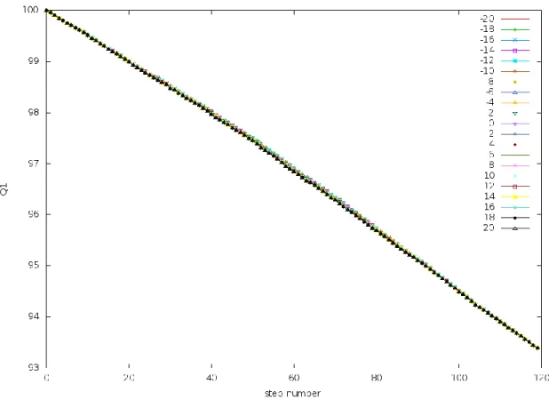
This means that the trajectory is only a linear interpolation between the initial and final states. Also, there is no dependence on Δ𝐸. This is demonstrated in Fig. 5, where the similarity of a state on the trajectory with respect to the initial state, 𝑄1, is plotted as a function of time. It
28
Figure 5. 𝑸𝟏 vs. t at small 𝒕𝒇:𝑄1 of a frame of the trajectory is the similarity of that frame to the
initial state of the trajectory. These trajectories were generated by simulating the PreTS to Pdt transition
of the TrpRS system (described later) at 𝑡𝑓=0.0003 at a range of Δ𝐸 values. The similarity metric
increases almost linearly with respect to time. This figure shows that the trajectory is a linear extrapolation
of the initial state. Also there is no dependence on Δ𝐸.
This behavior at low values of 𝑡𝑓 arises from the fact the system doesn’t have enough
time to undergo motion based on the potential and the equations of motion. Since the system is forced to reach the final state at 𝑡𝑓 and yet not enough time to given, the system changes its
conformation by a linear interpolation method. This linear interpolation is called morphing.
3.1.2 Intermediate values of 𝑡𝑓
The problem with small values of 𝑡𝑓 doesn’t affect the system in the intermediate regime
29
to define the boundaries of this regime. There is no special value of 𝑡𝑓 which works better than
others. But what is clear from the plot is that the dependence of the trajectory on the equations of motion and on Δ𝐸 reappears in this regime. The value of 𝑘𝑡 at which the ratio is the sinh terms is greater than the ratio of the time values is about 0.3. Since there is no special value of 𝑡𝑓, even though the trajectories are more reasonable than those in the small 𝑡𝑓 regime, this
regime is not particularly useful in identifying the optimum values of the PATH parameters.
Figure 6. 𝑸𝟏 vs. 𝒕 at intermediate values of 𝒕𝒇:𝑄1 of a frame of the trajectory is the similarity of
that frame to the initial state of the trajectory. These trajectories were generated by simulating the PreTS
to Pdt transition of the TrpRS system (described later) at 𝑡𝑓=30 at a range of Δ𝐸 values. The trajectories
at intermediate regime show dependence on Δ𝐸 and the 𝑄1 values have a sigmoidal dependence on
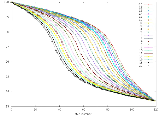
30 3.1.3 Large values of 𝑡𝑓
As shown by Figs. 5 and 6, with increase in 𝑡𝑓 the dependence on Δ𝐸 and on the sinh
terms of the equations of motion reappear.
Figure 7. 𝑸𝟏 vs. 𝒕 at large values of 𝒕𝒇:𝑄1 of a frame of the trajectory is the similarity of that
frame to the initial state of the trajectory. These trajectories were generated by simulating the PreTS to
Pdt transition of the TrpRS system (described later) at 𝑡𝑓=300 at a range of Δ𝐸 values. The sigmoidal
curves that were observed in the intermediate regime become steeper in the large 𝑡𝑓 regime. Also at Δ𝐸
values that are farther away from 0, the sigmoidal curves start to resemble a step function. This happens
because in the large regime, the step size used in plotting the curve might be too large and the entire
31
In this regime, the system has enough time to undergo transition under the influence of the equations of motion and the potential. Also, the convergence surface equation can be
solved at 𝑡̅ =𝑡𝑓
2 to get Δ𝐸0.5 as
Δ𝐸0.5= (𝐸𝑟𝑖𝑔ℎ𝑡− 𝐸𝑙𝑒𝑓𝑡) (
−𝑘𝑟𝑘𝑙 (𝑘𝑟+ 𝑘𝑙)2
) (50)
It is interesting to note that when 𝑘𝑟= 𝑘𝑙,
lim 𝑡𝑓→∞
Δ𝐸0.5 = − lim 𝑡𝑓→0
Δ𝐸0.5 (51)
Another observation that lends support to the hypothesis that using a large value of 𝑡𝑓 to
compute the trajectories is the correct approach, comes from the values of action. Since PATH is based on the minimization of the Onsager-Machlup action to derive the equations of motion, it is not surprising that the values of action might provide useful information for the optimization of PATH input parameters on the convergence surface.
For a double well system, the action of the most probable path in both the wells can be written as
𝑆 = 1
2𝛾(∫ (𝑚𝛾𝑥̇ + 𝑘𝑙(𝑥 − 𝑎))
2
𝑑𝑡 + ∫ (𝑚𝛾𝑥̇ + 𝑘𝑟(𝑥 − 𝑏))
2 𝑑𝑡 𝑡𝑓 𝑡̅ 𝑡̅ 0 ) (52)
Integrating the above equation for the left well is straight forward. On assuming that at time 𝑡 = 0, 𝑥 = 𝑎 and at 𝑡 = 𝑡̅, 𝑥 = 𝑥̅ then the equation for the action in the left well is
𝑆𝑙 = Γl
2(𝑥̅ − 𝑎)
2 𝑒Γl𝑡̅ sinh(𝛤𝑙𝑡̅)
(53)
32
In the right well, when the reaction is moving forward in time, the assumption that is made is that at time 𝑡 = 𝑡̅, 𝑥 = 𝑥̅ and at 𝑡 = 𝑡𝑓, 𝑥 = 𝑏. This assumption leads to the following
equation
𝑆𝑟 = Γr
2(𝑥̅ − 𝑏) 2 𝑒
−Γr(𝑡𝑓−𝑡̅)
sinh (𝛤𝑟(𝑡𝑓− 𝑡̅))
(54)
At large 𝑡𝑓 the two action equations give rise to Fig. 8. It can be seen from the figure that
33
Figure 8. Action vs. 𝚫𝑬 with the old equation for right action: Simulations of transition from
rigor state to the prepowerstroke state of myosin VI converter domain (described later) were performed at
𝑡𝑓= 300000 at a range of Δ𝐸 values. Left, right and total action plotted as a function of Δ𝐸 at this constant
large value of 𝑡𝑓. The left action goes to zero at large positive Δ𝐸 values because the initial state has
almost the same energy as the transition state and most of the trajectory is in the right well. But right
action also goes to 0 which is not the expected behavior.
The reason behind this behavior of the right action arises from the nature of the
34
direction of time is forward. The system can move from the transition state towards the equilibrium state only when time is reversed.
This consideration of the direction of time and displacement from the equilibrium state means that the trajectory and action in the right well have to be computed from state 𝑏 to the transition state and then the time is reversed so that the overall reaction goes from state 𝑎 to 𝑏. This modification in the assumptions gives rise to following equation for the right action
𝑆𝑟 = Γr
2(𝑥̅ − 𝑏) 2 𝑒
Γr(𝑡𝑓−𝑡̅)
sinh (𝛤𝑟(𝑡𝑓− 𝑡̅))
(55)
35
Figure 9. Action vs. 𝚫𝑬 with the new equation for right action: Simulations of transition from
rigor state to the prepowerstroke state of myosin VI converter domain (described later) were performed at
𝑡𝑓= 300000 at a range of Δ𝐸 values. Left, right and total action plotted as a function of Δ𝐸 at this constant
large value of 𝑡𝑓. The modified right action gives rise to a minimum in total action at Δ𝐸0.5.
The minimum of action, when plotted as a function of 𝑡𝑓 exponentially decays and
reaches an asymptotic value (Fig. 10). This is the global minimum of action that occurs at large values of 𝑡𝑓 and at Δ𝐸0.5. As the value of action is related to the probability of a path, the global
36
Figure 10. Minimum of action vs. 𝒕𝒇: Simulations of transition from rigor state to the
prepowerstroke state of myosin VI converter domain (described later) were performed at different values
of 𝑡𝑓 and Δ𝐸. The minimum of action at each value of 𝑡𝑓 behaves asymptotically with respect to 𝑡𝑓. This
curve also fits to an exponential equation with a 𝑅2 of 0.99
Based on Fig. 10, it is clear that running simulations at large values of 𝑡𝑓 is beneficial
and it also gives the value of Δ𝐸 at which the simulation has to be performed. But there is still no informational generated by the PATH method about the values of the force constants. It could be argued that since the product of 𝑘𝑡 is what determines whether the value of 𝑡𝑓 used is
37
structure of the transition state becomes invariant at large values of 𝑡𝑓. This means that when
the action is at its global minimum, the structure of the transition state converges.
Even though large values of 𝑡𝑓 generate the global minimum of action and invariant
transition state structures, it gives rise to a new problem. At extremely large values of 𝑡𝑓, the
path spends most of its time near the equilibrium structures and uses only a fraction of the total time to change the conformation of the protein. Also, the system spends more time in the narrower (more energetic) well than in the wider well.This behavior contradicts statistical
mechanics. But, at the same time, once the conformational change starts, the system takes less time to climb up the potential well in the narrower well than in the wider well, which is consistent with statistical mechanics.
The origin of these behaviors can be understood in the following way. As described earlier, converting the equations of motion from those defined by classical action to those defined by OM action changes the fractional increment in position, 𝑥(𝑡), from an oscillatory motion to the hyperbolic sine function.As a consequence, the system invariably spends most of its time at the origin (i.e., at 𝑥(𝑡) = 𝑎) and commences its climb to the transition state after an inordinately long time. This problem of the system spending most of the time in the initial state has previously been observed (Faccioli et al. 2006; Ghosh et al. 2002; Pinski & Stuart 2010). A solution to this problem can be obtained by transforming the Lagrangian from the
38
For protein conformational changes, like domain motions that depend on large frequency rigid-body motions, I describe multiple lines of evidence that no essential information is lost by truncating the initial, invariant portion of the trajectory during which the structure does not change. To solve this problem, the system must be given just enough time for the transition state to converge and no more. Thus, the PATH trajectory must be truncated by beginning only when the system has moved away from a by at least 10% of the total distance between the equilibrium state and the transition state. This is an arbitrary choice; using 1% of the distance from the equilibrium state would change the resulting transition state almost imperceptibly.
An appropriate value of 𝑡𝑓 can be calculated for the 1D diatomic system in the following
way. Using the equation of motion in 1D in the left well, a general OM trajectory can be written as
𝑥(𝑡) = 𝑎 + (𝑥̅ − 𝑎)sinh(𝑘𝑡)
sinh(𝑘𝑡̅) (56)
when 𝑡𝑓 → ∞, (55) becomes
𝑥(𝑡) = 𝑎 + (𝑥̅ − 𝑎)𝑒−𝑘(𝑡̅−𝑡) (57)
Since the time of interest is the one at which the system has changed by at least 10%,
𝑒−𝑘(𝑡̅−𝑡) = 0.1 (58)
which gives,
𝑡̅𝑜𝑝𝑡= 𝑡̅ − 𝑡 =2.302
𝑘 (59)
There is a 𝑡̅𝑜𝑝𝑡 for each well and 𝑡 𝑓
𝑜𝑝𝑡
is the sum of the two. Thus from (59) the optimum
value of 𝑡𝑓 can be solved. By using this value of 𝑡𝑓 and 𝑡̅ in the velocity continuity equation the
invariant 𝑥̅ can be identified and the Δ𝐸0.5 can also be calculated. Since (59) relates the force
39
as errors in the values can be compensated by the use of 𝑡𝑓 that is appropriate for the chosen
force constant.
This equation directly computes 𝑡̅ for a 1D diatomic system but for multiatom systems in 3D, there are multiple interatomic interactions, and hence multiple force constants associated with the diagonalized Hessian matrix. Hence, the average force constant for a structure can calculated which is the average of the trace of the Hessian
𝑘̅ =𝑡𝑟(𝐻)
3𝑁 (60)
where, 𝑁 is the number of atoms. And (59) becomes
𝑡̅𝑜𝑝𝑡= 𝑡̅ − 𝑡 =2.302
40
CHAPTER 4: VALIDATION AND RESULT FROM PATH SIMULATIONS
To validate the new PATH algorithm, I compared the results from PATH with those from other simulation algorithms, namely the String Method (E et al. 2002a; Ovchinnikov et al. 2011) and ANMPathway (Das et al. 2014). I also performed Discrete Molecular Dynamics (DMD) simulations (Dokholyan et al. 1998; Ding et al. 2008; Shirvanyants et al. 2012) using the replica exchange algorithm (Sugita & Okamoto 1999) to see if the PATH transition states are at the saddle points of the conformational free energy landscapes. Finally, I compared the transition states from a signaling protein, a contractile protein, and an enzyme and found similar structural elements contributing to the energy barrier at the transition state.
4.1 PATH, ANMPathway and the String trajectories agree most closely with each other at their transition states
41
to zero (Fig. 11(b)). In the context of PATH, the structure whose corresponding potential energy difference is zero is, by definition, the transition state.
Figure 11. PATH vs. ANMPathway and String: The ANMPathway trajectory and the string
trajectories were compared with the PATH trajectory. In (a), I calculated the RMSD between the transition
state from the PATH trajectory and all the states along the ANMPathway trajectory. States 28–31 are
structurally similar to the PATH transition state. In (b), I calculated the potential energy (PE) of each state
in the ANMPathway trajectory with respect to the potential energy well of the initial and the final state and
their absolute difference was plotted. States 27–30 have the lowest potential energy difference, which
coincides with the states in (a). I performed a similar comparison between the string trajectory (G3c) and
42
and the same states also have the lowest potential energy difference, implying their proximity to the same
transition state.
I performed a similar analysis with the myosin conformational change trajectory from the ANMPathway method (Das et al. 2014). I found that when the PATH transition state is
compared with the ANMPathway trajectory the structures are the closest [root mean squared deviation (RMSD) 0.52 Å] near the transition state of the ANMPathway trajectory (Fig 11(c)). Similarly, the same group of structures have the absolute potential energy difference closest to zero (Fig 11(d)).
4.2 Discrete molecular dynamics replica exchange simulations verify that transition states identified by path are close to saddle points in the free energy surface connecting initial and final states
Previous work in the lab (Kapustina et al. 2007) has established that Bacillus Stearothermophilus Tryptophanyl-tRNA synthetase (TrpRS) passes through three distinct structural states:
an Open state that can be stabilized either by stoichiometric amounts of
tryptophan or by substoichiometric amounts of Mg•ATP (adenosine triphosphate)
a closed, Pre-TS, stabilized by stoichiometric amounts of Mg•ATP and a
tryptophan analog
a closed, Product state (Pdt), stabilized either by the bound intermediate
adenylate product, tryptophanyl-5’AMP, or by stable analogs thereof
43
different conformational transition state. Preliminary analysis with the PATH program had given us descriptive accounts of the two transitions.
Induced-fit proceeds by and early and higher energy barrier that matches the
behavior seen by MD simulations of the TrpRS monomer (Laowanapiban et al. 2009)
Catalysis proceeds by a later, lower barrier transition state in which the volume of
the tryptophan binding pocket assumes a minimum value immediately after the conformational transition state identified by PATH (Weinreb et al. 2014)
The earlier MD calculations relating to the Induced-fit transition were short, 10 ns simulations,and represented what appeared to be a slower conformational change. As MD simulations led to a confirmation of the results PATH had given for the Induced-Fit transition (Laowanapiban et al. 2009), I decided to see whether similar, but more detailed simulations might allow a more stringent test of results the PATH algorithm had given for the catalytic transition. As the catalytic transition represents what is likely a more rapid conformational change with a lower barrier, I carried out replica exchange calculations using DMD (Dokholyan et al. 1998; Shirvanyants et al. 2012; Ding et al. 2008) with sufficiently long equilibrations to appropriately sample the free energy surface connecting the Pre-TS and Pdt states.
bi-44
variate quadratic for the transition state, to the points between the two equilibrium states. These representative structures reflect the stable, equilibrium structures of the two states in the DMD force field (Ding & Dokholyan 2006; Shirvanyants et al. 2012) as obtained from the DMD simulations. They were then input as initial and final states to PATH.
Figure 12. Free energy surface from Replica exchange DMD: Free energy surfaces for the
fully liganded TrpRS monomer derived from DMD replica exchange computations and plotted as a
function of the two conformational angles, Twist and Hinge, which represent collective variables for the
catalytic conformational change derived by Kapustina (Kapustina & Carter 2006). The structures (2000
45
Distributions of the TrpRS Pre-transition state and Product derived from simulations initiated from the
Product state in the (harmonically restrained) presence of AMP, tryptophan, and pyrophosphate. (B)
Distributions of these two states in similar simulations without pyrophosphate and without restraining
potentials. In (A) and (B), the dark blue circles represent the free energy minima of the less populated
state fitted to a bivariate quadratic response surface. Light blue circles represent free energy minima
computed using the same approach for the more highly populated states. (C) Free energy surface
derived from (A). (D) A similar plot derived from (B). Blue spheres represent the initial and final states
input to PATH computations; red spheres represent the coordinates of the transition states produced by
PATH.
These calculations produced two notable results:
The apparent free energy difference between the Pre-TS and Product states
depends strongly on the presence of the bound product, pyrophosphate (PPi). If the PPi was retained in the binding pocket by a harmonic potential, the
equilibrium was far on the side of the Pre-TS state (Fig 12 (a)). On the other hand, if this potential (or constraints) mimicking PPi binding was relaxed or omitted, rapid PPi release is observed and the distribution of states exhibits higher probability towards product state (Fig. 12(B)). This behavior is especially interesting in view of the possibility that early release of orthophosphate following actin binding triggers the myosin V powerstroke (Ovchinnikov et al. 2010).
Transition states for the transitions with and without the harmonic potential
restraining the PPi output by PATH fall close to the coordinates of the saddle points of the respective energy surfaces (Figs. 12(C) and 12(D)).
4.3 Transition states identified by PATH display comparable rate-limiting structures in three different systems
46
the course of the work, I found it useful also to investigate PATH behaviors of other model systems, including the 1D system described above. Two well-defined protein conformational transitions – Ca2+ release by the Ca2+-binding domain of calmodulin and the converter domain of
myosin VI. These studies reveal a remarkable similarity in all three transition-states (Fig. 13). In each case, the rate-limiting conformational change involves re-packing of multiple aromatic side chains (Burley & Petsko 1985; Burley & Petsko 1986; Lanzarotti et al. 2011) associated with subtle rearrangements of the surrounding backbone chains. Such rearrangements are known to occur on a far slower timescale (𝜇𝑠 to ms (Skalicky et al. 2001)) than rotamer exchanges of aliphatic side chains in hydrophobic core regions.
Figure 13. Transition states of three different systems: Conformational transition state
structures for Calmodulin Ca2+-binding domain (A), Myosin VI converter domain rigor to Prepowerstroke
(B), and the TrpRS induced-fit (C) transition states. Aromatic residues that flip at the transition state are
highlighted in red. The initial state is 50% transparent, to distinguish the states before and after the