1
Report Prepared for:
National Oceanic and Atmospheric Administration/National Ocean Service Coast Survey Development Laboratory, Office of Coast Survey
Mesh Development, Tidal Validation, and Hindcast Skill Assessment of an ADCIRC Model for the
Hurricane Storm Surge Operational Forecast System on the
US Gulf-Atlantic Coast
Submitted by: In Association With:
Riverside Technology, inc. 2950 E. Harmony Road, Suite 390 Fort Collins, Colorado 80528 970.484.7573
i
TABLE OF CONTENTS
Table of Contents ... i
List of Figures ... iv
List of Tables ... ix
List of Acronyms and Abbreviations ... x
1. Executive Summary ... 11
2. Introduction ... 12
3. Mesh Development ... 13
3.1 Model Boundary ... 13
3.2 Topography and Bathymetry Data Sources ... 14
3.3 ADCIRC Mesh ... 15
3.4 Elevation Assignment ... 17
3.5 Datum Conversion ... 17
4. ADCIRC Model Development ... 19
4.1 Fort.15 Model Control File ... 19
4.2 Fort.13 Nodal Attribute File... 21
4.2.1 Primitive Weighting in Continuity Equation ... 21
4.2.2 Formulation of Land Use-Dependent Parameters ... 21
4.2.3 Land Use Data Sources ... 22
4.2.4 Manning’s n at Sea Floor ... 23
4.2.5 Surface Canopy Coefficient ... 23
4.2.6 Surface Directional Effective Roughness Length (z0) ... 23
5. Astronomical Tide Scenario ... 26
5.1 Harmonic Forcings and Validation Data ... 26
5.2 Astronomical Tide Validation ... 26
5.2.1 Harmonic Constituent Amplitude Skill ... 26
5.2.2 Harmonic Constituent Phase Skill ... 29
5.2.3 Effect of Advection Terms... 31
5.3 Overall Tidal Skill ... 33
6. Storm Hindcast Validation 35 6.1 Typical Model Setup ... 35
6.2 Ike (2008) ... 38
ii
6.2.2 Results and Skill Assessment... 39
6.3 Katrina (2005) ... 47
6.3.1 Model Setup ... 47
6.3.2 Results and Skill Assessment... 48
6.4 Dennis (2005) ... 52
6.4.1 Model Setup ... 52
6.4.2 Results and Skill Assessment... 53
6.5 Charley (2004) ... 58
6.5.1 Model Setup ... 58
6.5.2 Results and Skill Assessment... 59
6.6 Hugo (1989) ... 64
6.6.1 Model Setup ... 64
6.6.2 Results and Skill Assessment... 65
6.7 Floyd (1999) ... 71
6.7.1 Model Setup ... 71
6.7.2 Results and Skill Assessment... 74
6.8 Isabel (2003) ... 78
6.8.1 Model Setup ... 78
6.8.2 Results and Skill Assessment... 79
6.9 Sandy (2012) ... 84
6.9.1 Model Setup ... 84
6.9.2 Results and Skill Assessment... 85
6.10 Long Island Express (1938) ... 92
6.10.1 Model Setup ... 92
6.10.2 Results and Skill Assessment... 93
6.11 Perfect Storm (1991) ... 98
6.11.1 Model Setup ... 98
6.11.2 Results and Skill Assessment... 99
7. Results for All Hindcast Events ... 104
8. Conclusions and Recommended Next Steps... 110
9. Acknowledgments ... 114
10. References ... 115
iii
11.1 ADCIRC Mesh Boundary Data Sources ... 118
11.2 ADCIRC Mesh Boundary Development and Modification ... 119
11.3 Connections with River Models ... 127
12. APPENDIX B – Development of Topo-Bathy Data and of Mesh ... 135
12.1 Data Sources ... 135
12.2 Datum Conversion ... 139
12.3 Meshing Methodology ... 141
12.4 Base Meshes ... 141
12.5 Flow Path Guidance ... 147
12.6 Flow Barrier Guidance ... 152
12.7 Topographic Peak Elevation Assignment ... 152
12.8 General Elevation Assignment ... 153
12.9 Final Mesh ... 153
12.9.1 NOMAD mesh topo-bathymetry ... 154
12.9.2 NOMAD mesh node spacing ... 161
13. APPENDIX C – List of Stations for Skill Assessment ... 167
iv
LIST OF FIGURES
Figure 3-1: Final mesh boundary in green with approximate 10-meter contour along US
inland boundary and EC2012 Mesh boundary elsewhere...14
Figure 3-2: Overview of final NOMAD mesh topo-bathymetry (feet MSL) ...16
Figure 3-3: Detail of NOMAD mesh topo-bathymetry (feet MSL) for US coastline. ...17
Figure 3-4: EC2012 mesh nodes shown in yellow and red. Red mesh nodes are those
within the extent of the extended VDatum conversion grid. ...18
Figure 5-1: Geographic distribution of M
2constituent amplitude error. ...27
Figure 5-2: Modeled versus predicted harmonic amplitudes for seven primary harmonic
constituents. ...28
Figure 5-3: Sorted relative amplitude error for seven primary harmonic constituents at
stations with M
2amplitude greater than 0.1 meters. ...28
Figure 5-4: Geographic distribution of phase error for M
2harmonic constituent. ...29
Figure 5-5: Correlation of modeled versus predicted harmonic phases. ...30
Figure 5-6: Sorted phase error for individual harmonic constituent phases. ...30
Figure 5-7: Water elevation solution at one time step 4 days before fatal instability. ...31
Figure 5-8: Correlation of M
2constituent amplitude comparing predicted and simulated
results from simulations with non-linear advection terms turned on (blue
points) and off (red points). ...32
Figure 5-9: A pseudo-geographic depiction of the effect of modification of the non-linear
advection; results from simulations with non-linear advection terms turned
on are plotted as blue points and off as red points. ...33
Figure 5-10: Geographic distribution of water level time series RMSE at 398 tide gages,
highlighting points exceeding the 0.2 meter RMS error metric...34
Figure 6-1: Approximate landfall locations of hindcast validation events. ...37
Figure 6-2: Storm track of Hurricane Ike. Dots denote 6-hour intervals and landfall. ...38
Figure 6-3: Ike maximum wind speeds (top, mph) and maximum modeled surge (bottom,
ft MSL); NOAA gage sites marked by pinwheels (bottom). ...39
Figure 6-4: Geographic distribution of NOAA gage peak surge error (feet, modeled
minus measured). ...40
Figure 6-5: Geographic distribution of NOAA gage time series RMSE (feet). ...41
Figure 6-6: Galveston area NOAA gage time series peak water level error (left, feet,
modeled minus measured) and RMSE (right, feet). ...41
Figure 6-7: Alongshore plot of time series RMSE at NOAA stations; selected stations
named for reference, red line indicates target RMSE, green line gives gage
mean RMSE, and the purple line is mean RMSE from all storms. ...42
Figure 6-8: Difference in peak surge for 1.04x winds from 1.09x winds (feet). ...43
Figure 6-9: Measured and modeled time series at Galveston Pleasure Pier, Texas. ...44
Figure 6-10: Measured and modeled time series at Bay Waveland, Mississippi. ...44
Figure 6-11: Measured and modeled time series at Galveston Bay Entrance, Texas. ...45
Figure 6-12: Measured and modeled time series at Galveston Pier, Texas. ...45
Figure 6-13: Ike advection-on minus advection-off peak surges (feet). ...46
Figure 6-14: Storm track of Hurricane Katrina. Dots denote 6-hour intervals and landfall. ...47
v
Figure 6-16: Geographic distribution of peak water level error (left) and time series
RMSE (right) at NOAA stations. Peak surge errors are only shown for
gages with a distinct surge signal...49
Figure 6-17: Alongshore plot of time series RMSE at NOAA stations; selected stations
named for reference; red line indicates target RMSE, green line gives gage
mean RMSE, and the purple line is mean RMSE from all storms. ...49
Figure 6-18: Measured and modeled time series at Waveland, Mississippi. ...50
Figure 6-19: Measured and modeled time series at Dauphin Island, Alabama. ...50
Figure 6-20: Katrina advection-on minus advection-off peak water level (feet). ...51
Figure 6-21: Storm track of Hurricane Dennis. Dots denote 6-hour intervals and landfall. ...52
Figure 6-22: Dennis maximum wind speeds (top, mph) and maximum modeled surge
(bottom, feet MSL); NOAA gage sites marked by pinwheels (bottom). ...53
Figure 6-23: Geographic distribution of peak water level error (left) and time series
RMSE (right) at NOAA stations. Peak surge errors are only shown for
gages with a distinct surge signal...54
Figure 6-24: Alongshore plot of time series RMSE at NOAA stations; selected stations
named for reference, red line indicates target RMSE, green line gives gage
mean RMSE, and the purple line is mean RMSE from all storms. ...55
Figure 6-25: Measured and modeled time series at Cedar Key, Florida. ...55
Figure 6-26: Measured and modeled time series at Apalachicola, Florida. ...56
Figure 6-27: Measured and modeled time series at Panama City, Florida. ...56
Figure 6-28: Comparison of measured HWMs vs. FEMA study modeled peak water
level] (left) and the same HWMs vs. NOMAD modeled peak water levels
(right). The NOMAD results shown are from a test run using with 1.09x
scaled winds for more direct comparison to the FEMA results. ...57
Figure 6-29: Dennis advection-on minus advection-off peak surges (feet). ...57
Figure 6-30: Storm track of Hurricane Charley. Dots denote 6-hour intervals and landfall. ...58
Figure 6-31 Charley maximum wind speeds (left, mph) and maximum modeled surge
(right, feet MSL); NOAA gage sites marked by pinwheels (right). ...59
Figure 6-32 Geographic distribution of peak water level error (left) and time series
RMSE (right) at NOAA stations. Peak surge errors are only shown for
gages with a distinct surge signal...60
Figure 6-33 Measured and modeled time series at Loggerhead Key, Florida. ...60
Figure 6-34 Measured and modeled time series at Fort Meyers, Florida. ...61
Figure 6-35 Hurricane Charley surveyed post-storm HWMs (left) and HWM error (right). ...62
Figure 6-36: Charley advection-on minus advection-off peak surges (feet). ...63
Figure 6-37: Storm track of Hurricane Hugo. Dots denote 6-hour intervals. ...64
Figure 6-38 Hugo maximum wind speeds (left, mph) and maximum modeled surge (right,
feet MSL); NOAA gage sites marked by pinwheels (right). ...65
Figure 6-39 Geographic distribution of peak water level error (left) and time series
RMSE (right) at NOAA stations. Peak surge errors are only shown for
gages with a distinct surge signal...65
Figure 6-40 Alongshore plot of time series RMSE at NOAA stations; selected stations
named for reference; red line indicates target RMSE, green line gives gage
mean RMSE, and the purple line is mean RMSE from all storms. ...66
vi
Figure 6-42 Measured and modeled time series at Charleston, South Carolina. ...67
Figure 6-43: Post-storm HWM data error, modeled minus measured. ...68
Figure 6-44 Comparison of NOMAD vs. FEMA model skill to measured surge height. ...69
Figure 6-45 Peak water level difference (feet) showing NOMAD modeled minus FEMA
modeled values...69
Figure 6-46: Hugo advection-on minus advection-off peak surges (feet). ...70
Figure 6-47: Storm track of Hurricane Floyd. Dots denote 6-hour intervals...71
Figure 6-48: Floyd H*Wind and Best track maximum wind speed (left and right,
respectively, kilometers per hour) ...72
Figure 6-49: H*Wind maximum modeled surge (bottom left and bottom right,
respectively, meters MSL) ...73
Figure 6-50: Differences between advection-on and advection-off simulations using the
H*Wind forcing data for Floyd. ...73
Figure 6-51: Geographic distribution of peak water level error (left) and time series
RMSE (right) at NOAA stations. Peak surge errors are only shown for
gages with a distinct surge signal...74
Figure 6-52: Alongshore plot of time series RMSE at NOAA stations; selected stations
named for reference; red line indicates target RMSE, green line gives gage
mean RMSE, and the purple line is mean RMSE from all storms. ...75
Figure 6-53: Observed and simulated water levels during Floyd at Money Point, VA.
Green is observed (obs); dark blue is advection-off H*Wind (flr01); light
blue is advection-on H*Wind (flr02); black is best track (flr03)...76
Figure 6-54: Observed and simulated water levels during Floyd at Cape Hatteras, NC.
Green is observed (obs); dark blue is advection-off H*Wind (flr01); light
blue is advection-on H*Wind (flr02); black is best track (flr03)...76
Figure 6-55: Observed and simulated water levels during Floyd at Atlantic Beach, NC.
Green is observed (obs); dark blue is advection-off H*Wind (flr01); light
blue is advection-on H*Wind (flr02); black is best track (flr03)...76
Figure 6-56: Observed and simulated water levels during Floyd at Wilmington, NC.
Green is observed (obs); dark blue is advection-off H*Wind (flr01); light
blue is advection-on H*Wind (flr02); black is best track (flr03)...77
Figure 6-57: Observed and simulated water levels during Floyd at Springmaid Pier, SC.
Green is observed (obs); dark blue is advection-off H*Wind (flr01); light
blue is advection-on H*Wind (flr02); black is best track (flr03)...77
Figure 6-58: Observed and simulated water levels during Floyd at St. Simons Island, GA.
Green is observed (obs); dark blue is advection-off H*Wind (flr01); light
blue is advection-on H*Wind (flr02); black is best track (flr03)...77
Figure 6-59: Storm track of Hurricane Isabel. Dots denote 6-hour intervals and landfall. ...78
Figure 6-60: Isabel maximum wind speeds (left) and maximum modeled surge (left);
NOAA gage sites marked by pinwheels (right). ...79
Figure 6-61: Geographic distribution of peak water level error (left) and time series
RMSE (right) at NOAA stations. Peak surge errors are shown only for
gages with a distinct surge signal...80
Figure 6-62: Alongshore plot of time series RMSE at NOAA stations; selected stations
named for reference; red line indicates target RMSE, green line gives gage
vii
Figure 6-63: Measured and modeled time series at Washington, DC. ...81
Figure 6-64: Measured and modeled time series at Newbold, Pennsylvania. ...82
Figure 6-65 Measured and modeled time series at Oregon Inlet Marina, North Carolina. ...82
Figure 6-66: Measured and modeled time series at Cape Hatteras Fishing Pier, North
Carolina. ...83
Figure 6-67: Storm track of Hurricane Sandy. Dots denote 6-hour intervals, extratropical
transition, and landfall. ...84
Figure 6-68 Sandy maximum wind speeds (top, mph) and maximum modeled surge
(bottom, feet MSL); NOAA gage sites marked by pinwheels (bottom). ...85
Figure 6-69 Geographic distribution of peak water level error (left) and time series
RMSE (right) at NOAA stations. HWM errors are limited to gages with a
distinct surge signal...86
Figure 6-70 Alongshore plot of time series RMSE at NOAA stations; selected stations
named for reference; red line indicates target RMSE, green line gives gage
mean RMSE, and the purple line is mean RMSE from all storms. ...86
Figure 6-71: Measured and modeled time series at Providence, Rhode Island. ...87
Figure 6-72: Measured and modeled time series at New Haven, Connecticut. ...87
Figure 6-73 Measured and modeled time series at Kings Point, New York...88
Figure 6-74: Measured and modeled time series at The Battery, New York. ...88
Figure 6-75: Measured and modeled time series at Bergen Point, New York. ...89
Figure 6-76: Measured and modeled time series at Sandy Hook, New Jersey. ...89
Figure 6-77 Measured and modeled time series at Atlantic City, New Jersey. ...90
Figure 6-78 Measured and modeled time series at Cape May, New Jersey. ...90
Figure 6-79 Measured and modeled time series at Ocean City, Maryland. ...91
Figure 6-80: Storm track of the Long Island Express. Dots denote 6-hour intervals and
landfall. ...92
Figure 6-81 Long Island Express maximum wind speeds (top, mph) and maximum
modeled surge (bottom, feet MSL; NOAA gage sites marked by pinwheels
(bottom)...93
Figure 6-82 Geographic distribution of peak water level error (left) and time series
RMSE (right) at NOAA stations. HWM errors are limited to gages with a
distinct surge signal...94
Figure 6-83: Geographic distribution of peak water level error from additional high water
marks. ...94
Figure 6-84 Alongshore plot of time series RMSE at NOAA stations; selected stations
named for reference; red line indicates target RMSE, green line gives gage
mean RMSE, and the purple line is mean RMSE from all storms. ...95
Figure 6-85 Measured and modeled time series at Willets Point, New York. ...96
Figure 6-86 Measured and modeled time series at The Battery, New York. ...96
Figure 6-87: Long Island Express advection-on minus advection-off peak surges (feet). ...97
Figure 6-88: Storm track of the Perfect Storm. Dots denote 6-hour intervals. ...98
viii
Figure 6-90: Geographic distribution of peak water level error (left) and time series
RMSE (right) at NOAA stations. HWM errors are limited to gages with a
distinct surge signal...100
Figure 6-91: Alongshore plot of time series RMSE at NOAA stations; selected stations
named for reference; red line indicates target RMSE, green line gives gage
mean RMSE, and the purple line is mean RMSE from all storms. ...101
Figure 6-92: Measured and modeled time series at Woods Hole, Massachusetts. ...101
Figure 6-93: Measured and modeled time series at Montauk, New York. ...102
Figure 6-94 Comparison of NOMAD (top) to FEMA (bottom) time series at Atlantic
City, New Jersey. ...103
Figure 7-1: NOAA gage time series RMSE for all storms. ...105
Figure 7-2: NOAA gage mean water level difference for all storms. ...105
Figure 7-3: Along-shore NOAA gage time series RMSE for all storms. ...106
Figure 7-4: Along-shore NOAA gage time series mean difference for all storms. ...106
Figure 7-5 Peak water level error and surveyed HWM error for all storms. Data points
labeled ‘extra’ are surveyed HWM datasets for the corresponding events ...107
Figure 7-6: Along-shore NOAA gage peak water level error. ...107
Figure 7-7: Peak water level and surveyed HWM comparison for all storms. Data points
labeled ‘extra’ are surveyed HWM datasets for the corresponding events. ...108
Figure 7-8 Sorted RMSEs from all NOAA gages (excluding gages which failed during
the event) across all validation storm simulations. Gages used in multiple
storms have multiple points. ...109
ix
LIST OF TABLES
Table 4-1: ADCIRC Control File Parameters ...20
Table 4-2: Mapping of Spatial Parameters to CCAP Classes ...24
Table 4-3: NLCD Land Use Classifications ...25
Table 6-1: Summary of tropical and extratropical cyclone hindcast validation simulations. ...36
Table 6-2: Comparison of HWM Error. ...102
Table 12-1: Sources of topo-bathymetric data for development of the HSSOFS mesh
node elevations...136
x
LIST OF ACRONYMS AND ABBREVIATIONS
ADCIRC ADvanced CIRCulation model
CO-OPS Center for Operational Oceanographic Products and Services CSDL Costal Survey Development Laboratory
ETSS Extratropical Storm Surge
ESTOFS Extratropical Surge and Tide Operational Forecast System
FEMA Federal Emergency Management Agency
GFS Global Forecast System
EC2012 East Coast 2012 Tidal Constituent Project
HWM High Water Mark
MSL Mean Sea Level
MLLW Mean Lower Low Water
NCEP National Centers for Environmental Prediction
NHC National Hurricane Center
NOS National Ocean Service
NOAA National Oceanic and Atmospheric Administration
NWS National Weather Service
NAVD 88 North American Vertical Datum of 1988
OCS Office of Coast Survey
OPC Ocean Prediction Center
RMSE Root Mean Square Error
11
1.
EXECUTIVE SUMMARY
The Coast Survey Development Laboratory (CSDL) of the National Ocean Service (NOS) previously developed an Extratropical Surge and Tide Operational Forecast System (ESTOFS) for the US coastal waters (Funakoshi et al. 2013). Now, to extend the capability of ESTOFS to include tropical storm event simulation and ensemble prediction, CSDL is preparing a prototype Hurricane Storm Surge Operational Forecast System (HSSOFS). Under direction from CSDL, a technical team led by Riverside Technology, inc. has developed a hydrodynamic model of the US East Coast and Gulf of Mexico and has validated the model for 10 major tropical and extratropical events. Eventually, this model will form the basis for an operational system on National Centers for Environmental Prediction (NCEP) computers. The prototype model described in this document is called NOMAD: NOAA Operational Model with ADCIRC.
The hydrodynamic model employed for NOMAD is the ADvanced CIRCulation (ADCIRC) finite element model (Luettich et al. 1992; Luettich and Westerink 2004). The ADCIRC hydrodynamic model has demonstrated to be effective at predicting tidal circulation and storm surge propagation in complex coastal systems.
For the development of NOMAD, the project team constructed a new model grid covering all of the US Atlantic and Gulf coasts. Two model-run scenarios were tested: 1) astronomical tide and 2) model
hindcast. The model results from each scenario are compared with observations using NOS’ standard skill assessment software. The skill assessment demonstrated that NOMAD generally predicts the surge reasonably well, considering the meteorological forcing.
The target error metric was 0.2 meters RMSE (0.66 feet). With no adjustment for mean water level differences, the mean RMSE for all storms is about 0.26 meters (0.85 feet) with a range from
12
2.
INTRODUCTION
Impacts of storm surge from extratropical and tropical events can be far-reaching and catastrophic along the coast of the United States. The Office of Coast Survey/CSDL (OCS/CSDL) of the NOS and the Environmental Modeling Center (EMC) of NCEP have previously collaborated to establish an ESTOFS for the Atlantic and Gulf of Mexico (Funakoshi et al. 2013).
Continuing in the path of the ESTOFS development, CSDL has established an objective to further improve operational storm surge guidance for Eastern and Gulf US coasts. The objective includes
providing guidance during both extratropical and tropical surge events, providing ensemble forecasts, and preparing to address the effects of combined coastal and river flooding by expanding into key areas of interest for coupled river-ocean modelling. To accomplish these goals, CSDL is developing a new hydrodynamic model which will be implemented for operational simulations of storm surge and ocean water levels due to both tropical and extratropical storm events.
The hydrodynamic model code employed will be the ADvanced CIRCulation (ADCIRC) finite element model (Luettich et al. 1992; Luettich and Westerink 2004). ADCIRC has proven effective at predicting tidal circulation and storm surge propagation in complex coastal systems. Its unstructured grid
methodology allows for representation of complex shorelines and bathymetry.
CSDL tasked a team (‘the Project Team’ or ‘the Team’) from Riverside Technology, inc. (Riverside) and AECOM (formerly URS Group, Inc.) to:
Develop a preliminary ADCIRC mesh based on best-available bathymetry and overland topography.
Validate the preliminary model mesh using tidal harmonics.
Execute hindcast simulations of 10 significant historical tropical and extratropical storm events. Evaluate model hindcast performance using both the NOS standard skill assessment program
(Zhang et al. 2006) and criteria (Hess et al. 2003), as well as comparison to observed high water marks.
This report describes the work performed to develop and validate the preliminary ADCIRC model, which is referred to herein as the NOAA Operational Model with ADCIRC (NOMAD). When implemented operationally with appropriate meteorological forcing, and following additional testing and verification by CSDL, the new model is expected to be called the Hurricane Storm Surge Operational Forecast System (HSSOFS).
13
3.
MESH DEVELOPMENT
CSDL will use the NOMAD mesh as a basis for HSSOFS to provide operational surge and tide predictions for the US East Coast and Gulf of Mexico. The ADCIRC unstructured mesh allows
simulation for such a large domain, while still providing resolution of local coastal features. Given that the application of interest includes overland flooding, both topographic and bathymetric data sources were collected to prepare the model. The final mesh averages node spacing of 500 meters along the coast with some areas decreasing to a node spacing of approximately 150 meters. There are a total of approximately 1.8 million nodes.
CSDL provided mesh datasets which were used for various purposes during this project including various versions of the East Coast tidal constituent simulation meshes (EC2001, EC2001Ex, and EC2012). CSDL also provided access to a detailed mesh developed by researchers at University of Notre Dame for storm surge studies in Puerto Rico and the US Virgin Islands. Finally, a set of mesh datasets for coastal
Louisiana and Mississippi were provided by CSDL from inland surge models developed in collaboration with the Southeastern Universities Research Association (SURA) and the Integrated Ocean Observation System (IOOS). Additional detail and references for datasets used to define the model boundary and facilitate mesh development are contained in Appendix A and Appendix B.
3.1
Model Boundary
The inland mesh boundary was developed following these general guidelines:
At most locations, the mesh extends inland to a smoothed version of the 10-meter topographic contour.
In some areas with major population centers, the mesh was extended inland beyond the 10-meter topographic contour to include the entire developed area in the final mesh.
Except for significant rivers to be considered for coupled modeling, the boundary extends into coastal river inlets only to the point where the channel width decreases below approximately 1,500 meters.
In some areas where the 10-meter contour was significantly inland of the Federal Emergency Management Agency (FEMA) determined 0.2-percent-annual-chance flood elevation, the amount of modeled inland area was reduced.
The SURA-IOOS mesh for portions of Texas, Louisiana, and Mississippi provided the mesh boundary in those areas.
Portions of the Everglades, though well below the 10-meter contour, were specifically excluded from the mesh because of low population, complex flow dynamics, and the presence of levees. Non-US overland areas are excluded from the mesh. Coastal boundaries outside of the United
States are from the EC2012 Mesh boundary.
All of the ESTOFS-modeled area is included in the new mesh.
Understanding the long-term objective of integrating the water level forecast from HSSOFS with riverine water level forecasts, the team reviewed a number of areas along the Atlantic and Gulf coasts where the NWS is developing riverine HEC-RAS models. The following river inlets were identified for inclusion in the NOMAD mesh: the Atchafalaya, Mississippi, St. John’s, Waccamaw, Tar, Potomac, Hudson, and Connecticut rivers.
The open ocean boundary location for the model coincides with the EC2001 extended mesh developed by the University of Oklahoma. This selection allowed for direct application of a number of existing datasets developed for that boundary and provided by NOAA for this project. The mesh model boundary is seen in Figure 3-1.
14
Figure 3-1: Final mesh boundary in green with approximate 10-meter contour along US inland boundary and EC2012 Mesh boundary elsewhere.
3.2
Topography and Bathymetry Data Sources
15
3.3
ADCIRC Mesh
Attention to mesh quality is essential to produce a geometry that not only accurately represents the terrain and bathymetry, but also produces stable and consistent results when run with the ADCIRC model. The ADCIRC model runs on a triangulated mesh with varying element sizes. Each node has an associated elevation. Additional spatial parameters can also be associated with each node. Due to the large
geographic extent of this project including the Atlantic and Gulf of Mexico, the mesh was constructed in separate sections by different team members using a guiding methodology to maintain consistency throughout the study domain.
One key mesh development constraint, derived from the intended operational implementation of the model, included maintaining a total node count of less than 2,000,000 nodes. An average spacing was defined in the US near shore and onshore areas of around 400 to 500 meters with a nominal minimum spacing around 200 meters for smaller channels, specifically where flow paths tie together large water bodies, or provide a conduit to extensive inland flooding behind major flow barriers. Some highly populated areas were also modeled with a finer-scale mesh.
The mesh extent was generated from several sources, including developing much of the over-land mesh in-house. For this task, the high-resolution topographic data sources referenced in Section3.2 were carefully examined to identify locations of critical flow pathways and flow barriers. The technical team traced break lines along these features and provided the break lines to the meshing algorithm to explicitly include the features in the mesh. In addition, the team examined data extracted from the National Levee Database to confirm the location of levees were properly represented within the study area. CSDL
provided the technical team with several mesh geometries including the NOAA EastCoast 2012 (EC2012) tidal constituent database mesh and the Extended EastCoast2001 (ExEC2001) mesh. Both geometries cover the entire deep-ocean domain. The EC2012 mesh has more than two million nodes while the ExEc2001 mesh has approximately 258,000 nodes.
In addition, CSDL provided the Gulf Coast-focused SURA-IOOS mesh developed for round one of the Coastal Ocean Modeling Testbed project. Generally, the SURA-IOOS mesh had less dense node spacing than what was developed for other areas on the Gulf and Atlantic coasts, but it remains useful because it was specifically designed and tested for storm surge studies in the Louisiana and Mississippi coasts. Because of the lower node spacing of this mesh (lower than other meshes used in Louisiana), it is also referred to as the Ultralite mesh, referring to the relatively lightweight computational load required for simulating larger node spacing.
The team also examined a mesh developed for detailed storm surge studies in Puerto Rico and the US Virgin Islands. The mesh, developed by Joannes Westerink and Juan Gonzales-Lopez from the University of Notre Dame, was more detailed than necessary for this project due to a minimum node spacing of 14 meters.
The final mesh incorporated all of the geometries detailed above, combined and edited to the appropriate resolution for the current modeling task. The node and element configuration from the on-shore and near-shore areas of the SURA-IOOS mesh for Louisiana and Mississippi was incorporated with minor
modifications. The Puerto Rico mesh was indirectly incorporated, as the inland boundary was extracted and then smoothed using a large node-to-node spacing. This boundary was used to develop the overland portion of the mesh for Puerto Rico and the US Virgin Islands. The smaller node count ExEC2001 mesh was used directly for the deep ocean boundary, and the EC2012 mesh nodes were used as a bathymetry data source for the near shore as explained below.
16
Atlantic. Figure 3-2 gives an overview of the final mesh topo-bathymetry followed by Figure 3-3 showing greater detail for the US coast. Additional detail images showing bathymetry and mesh node spacing for select areas are found in Appendix B.
17
Figure 3-3: Detail of NOMAD mesh topo-bathymetry (feet MSL) for US coastline.
3.4
Elevation Assignment
For broad overland areas exclusive of explicit barriers or channels, the topographic data was smoothed using a circular averaging window with a radius of 100 to 300 meters via ArcGIS focal statistics. A Fortran program was then used to assign elevations from the closest elevation data point in the smoothed topographic DEM to each mesh node
3.5
Datum Conversion
As previously noted, the EC2012 mesh node elevations are the primary source for bathymetric data for building the storm surge modeling mesh. It was necessary to convert the node elevations from MSL to NAVD88 in order to combine them with topographic data from the USGS. Normally, a translation of this type would be performed using the NOS-provided tool, VDatum. However, the VDatum application provided on the NOS website1 uses a translation grid with several key areas missing, including Pamlico Sound and the Indian River inlet.
CSDL provided an updated bathymetric translation grid that extends beyond the publicly available VDatum grid into all coastal waters within the model area of interest (Figure 3-4). The translation grid uses the TCARI interpolation technique (Hess et al. 2004) to allow extrapolation of the datum conversion field a significant distance over land and into the deep ocean. Where they overlap, the extended
conversion is identical to the VDatum grid conversion. Using CSDL code provided with the extended grid, a complete set of MSL-to-NAVD88 conversion values was generated for the entire near-shore bathymetric dataset from the EC2012 grid nodes.
18
A similar process was applied to convert the combined storm surge modeling mesh nodes back to MSL for use in modeling. When simulation results have been obtained, these conversion values will be applied as needed to compare to verification datasets in either MSL or NAVD88. The CSDL code was extremely efficient for converting the large point datasets represented by the mesh nodes.
19
4.
ADCIRC MODEL DEVELOPMENT
Each ADCIRC model is constructed with various control files to represent the mesh and forcing characteristics for a particular simulation. Except where specifically noted otherwise, all tidal and hindcast simulations for the NOMAD model reported here used fort.15 control files and fort.13 nodal attribute files conforming to the descriptions in the following sections.
4.1
Fort.15 Model Control File
The fort.15 file is the model control file used for setting physical parameters and determining how the model runs. Table 4-1 shows the parameters, their values and rationale for these values in the fort.15 ADCIRC control file. The parameter values were chosen to accurately represent system physics while ensuring simulations were stable.
Tidal forcing is applied as an elevation-specified boundary condition at the model’s oceanic boundary along the offshore boundary and as a body force on all nodes in the domain. Tidal forcing constituents were obtained from CSDL who specified them on the extended EC2001 mesh (whose boundary was adapted from the EC2012 mesh). The K1, K2, M2, N2, O1, Q1, S2, P1, Mf, Mm, M4, Ms4, and Mn4 constituents were used.
The ADCIRC model land boundary conditions prevent normal flow, but they do not restrict tangential flow. No river boundary conditions are specified in the study region, although several rivers, including the Potomac, Hudson, Mississippi, and Atchafalaya Rivers, are represented up to the mesh’s inland boundary.
20
Table 4-1: ADCIRC Control File Parameters
Parameter Description Value Explanation
NOLIBF Parameter controlling the type of bottom stress parameterization used in a two-dimensional depth-integrated (2DDI) ADCIRC run.
1 = quadratic bottom friction law.
1 Standard value. This value is necessary for using the
“mannings_n_at_sea_floor” nodal attribute in the fort.13 file. NOLIFA Parameter controlling the finite amplitude terms in
ADCIRC.
2 = finite amplitude terms are included in the model run and wetting and drying of elements is enabled.
2 Recommended value. This value has been used in previous studies, including the Big Bend study.
NOLICA Parameter controlling the advective terms in ADCIRC (with the exception of a time derivative portion that occurs in the GWCE form of the continuity equation). 1 = advective terms are included in the computations.
0 or 1 1 when possible, though some simulations were unstable.
NOLICAT Parameter controlling the time derivative portion of the advective terms that occurs in the GWCE form of the continuity equation in ADCIRC.
1 = the time derivative portion of the advective terms that occur in the GWCE continuity equation are included in the computations.
0 or 1 1 when possible, though some simulations were unstable.
NCOR Parameter controlling whether the Coriolis parameter is spatially varying as computed from the
y-coordinates of the nodes in the grid.
1 = compute a spatially variable Coriolis parameter.
1 Standard recommended value. This value is most representative of the system physics.
TAU0 Generalized Wave Continuity Equation (GWCE) weighting factor that weights the relative contribution of the primitive and wave portions of the GWCE. A value of -3 indicates that the value varies in space and time according to the nodal attribute
“primitive_weighting_in_continuity_equation.”
-3 Standard value. See Section 4.2.1 for more information.
DTDP ADCIRC time step (in seconds). 2 Model was also generally stable at 4 seconds.
A00, B00, C00
Time weighting factors (at time levels k+1, k, k-1, respectively) in the GWCE.
0.35, 0.3, 0.35
Standard value.
H0 Nominal water depth for a node (and the
accompanying elements) to be considered dry (in meters).
0.05 Value within the recommended range of 0.01 to 0.1 m.
VELMIN Minimum velocity for wetting (in meters per second). 0.05 Standard recommended value. CF Minimum value of the equivalent quadratic friction
coefficient determined by Manning’s n value.
0.0025 Standard value used in other studies, including the Big Bend study.
ESLM Spatially constant horizontal eddy viscosity for the momentum equations (units of length2/time).
21
4.2
Fort.13 Nodal Attribute File
The ADCIRC model is capable of applying multiple spatially varying parameters (nodal attributes), many of which alter wind and bottom drag using land use data. The following subsections detail the nodal parameters and the land use data used for the spatial attributes. All Fortran utilities used to create the various nodal attributes can be found on the ADCIRC website2.
4.2.1 Primitive Weighting in Continuity Equation
The “primitive weighting in continuity equation” attribute sets the τ0 parameter, controlling the relative contribution of the primitive and wave portions of the GWCE, which is a reformulation of the shallow water equation used by the ADCIRC model. This balance is such that for τ0, a value of 0 is the pure wave equation and a value greater than 1 behaves like a pure primitive continuity equation.
The program tau0_gen.f from the ADCIRC website was used to create the “primitive weighting in continuity equation” attribute. The parameter was set by finding the average distance between a node and its neighbors (as determined by the element connectivity between nodes). If the average distance between neighboring nodes was less than 1,750 meters, the τ0 parameter was set to 0.03. Otherwise, the value was set to 0.005 for depths greater than 10 meters and 0.02 for depths less than or equal to 10 meters. A value of 0.03 causes the ADCIRC model to calculate the τ0 parameter for each node at each time step
throughout the simulation using a hard-coded scheme. Details on the scheme are provided at the ADCIRC website3.
4.2.2 Formulation of Land Use-Dependent Parameters
The effect of spatially variable land cover and land use types enter into the computations via three coefficients. Three spatial variable parameters are applied in the bottom and surface stress terms in the depth averaged momentum equations:
𝜕𝑢 𝜕𝑡+ 𝑢
𝜕𝑢 𝜕𝑥+ 𝑣
𝜕𝑢
𝜕𝑦− 𝑓𝑢 = −𝑔 𝜕 𝜕𝑥(
𝑃
𝑔𝜌+ ζ) − 𝜏𝑏𝑥
𝜌𝐻+
𝜏𝑠𝑥
𝜌𝐻+
1
𝐻(𝑀𝑥+ 𝐷𝑥− 𝐵𝑥)
in the x-direction and
𝜕𝑣 𝜕𝑡+ 𝑢
𝜕𝑣 𝜕𝑥+ 𝑣
𝜕𝑣
𝜕𝑦+ 𝑓𝑣 = −𝑔 𝜕 𝜕𝑦(
𝑃
𝑔𝜌+ ζ) − 𝜏𝑏𝑦
𝜌𝐻+
𝜏𝑠𝑦
𝜌𝐻+
1
𝐻(𝑀𝑦+ 𝐷𝑦− 𝐵𝑦)
in the y-direction, where: t = time
x and y = horizontal spatial coordinates u and v = horizontal velocity vectors f = Coriolis parameter
P = pressure
ζ = free surface departure from the geoid H = total water column height
M = vertically integrated later stress gradient D = momentum dispersion
B = vertically integrated baroclinic pressure gradient g = the acceleration due to gravity
ρ = water density (1,000 kilograms/m3, about 1.94 slug/ft3) τb = bottom stress
τs = the surface stress
The bottom stress terms are approximated as:
2 http://adcirc.org/home/related-software/adcirc-utility-programs/.
22
𝜏𝑏𝑥
𝜌𝐻= 𝑔
𝑛2
𝐻13
√𝑢2+ 𝑣2
𝐻 𝑢
𝜏𝑏𝑦
𝜌𝐻 = 𝑔
𝑛2
𝐻13
√𝑢2+ 𝑣2
𝐻 𝑣
where n is the Manning’s n parameter, which is specified for every ADCIRC node as the “Manning’s n at sea floor” attribute. This parameter is applied to every node under the assumption that nodes anywhere in the mesh can become submerged as the storm surges propagate inland.
The surface stress terms are approximated as:
𝜏𝑠𝑥
𝜌𝐻=
𝐶𝑑
𝐻 𝜌𝑎𝑖𝑟
𝜌 |𝑊10|𝑊10𝑥 𝜏𝑠𝑦
𝜌𝐻=
𝐶𝑑 𝐻
𝜌𝑎𝑖𝑟
𝜌 |𝑊10|𝑊10𝑦
where Cd is a standard drag coefficient defined by Garratt’s drag formula (Garratt 1977) for wind stress, ρair is the density of air (1.15 kilograms/m3, about 0.00223 slug/ft3), and W10 is the wind velocity at a 10-meter height sampled at a 10-minute period (Hsu 1988). The W10 value is the wind velocity for full marine conditions as provided by an appropriate wind model (Powell et al. 1996). To account for the effect of land roughness, the 10-meter wind velocity is replaced by a reduced Wland velocity. The Wland velocity is found by:
𝑊𝑙𝑎𝑛𝑑= 𝑓𝑑∙ 𝑊10
where fd is the ratio of marine roughness to the roughness of the land surface and is expressed as:
𝑓𝑑= (
𝑧𝑚𝑎𝑟𝑖𝑛𝑒
𝑧0 )
0.0706
where zmarine and z0 are the marine and land roughness lengths, respectively; zmarine is defined as:
𝑧𝑚𝑎𝑟𝑖𝑛𝑒=
0.018
𝑔 𝐶𝑑𝑊102
The z0 length scale is specified at every node as the “surface directional effective roughness length” attribute. This length scale varies with land cover and has been determined for a variety of standardized land use classifications.
In addition to the Manning’s n and z0 parameters, a third parameter is used to represent the effects of tall and dense vegetation on the wind stress term. It has been shown that little wind momentum transfers through heavily forested canopies. The effect of forested vegetative canopies is included by reducing Wlandto zero in the presence of land use classes that contain trees and thick shrubs, and is specified as the “surface canopy coefficient” nodal attribute. This attribute represents the assumption that the branches, leaves, and trunks absorb the momentum of the wind, thereby preventing momentum transfer to the underlying water column.
4.2.3 Land Use Data Sources
The Manning’s n, surface roughness length and canopy coefficient parameters all depend on local land use information. It is standard practice to evaluate these parameters using land use classification data. The Coastal Change Analysis Program (CCAP) regional land cover data are a recent NOAA product4 and have been chosen to develop the frictional parameters. CCAP data define 22 land cover classes and
23
provide the spatial distribution of these classes across the study region at a resolution of 30 meters. Last updated in 2006, CCAP data are the most recent available source at the required resolution. The CCAP data were therefore chosen to help define model spatial attributes in the study area.
USGS National Land Cover Database (NLCD) data is also often used in surge modeling studies. NLCD data has a well-established set of values for the z0 parameter derived from Hazus (FEMA 2014; Vickery et al. 2006). Like NOAA’s CCAP data, the USGS Gap Analysis Program (GAP) land use data identify local habitat and biodiversity and have more accurate local detail and well-defined vegetation
subdivisions than the nationally uniform NLCD set. Standard hydraulic texts have helped establish bottom friction Manning’s n values for all the classifications in the GAP data. Each point in the CCAP data set has a class, and each class has an associated value for the needed parameters (Table 4-2). The spatially variable attributes for each ADCIRC node were obtained by interpolating parameter values from nearby CCAP data set points. The standard NLCD land use classification mapping is provided in Table 4-3 for comparison.
4.2.4 Manning’s n at Sea Floor
Manning’s n at sea floor is an isotropic scalar parameter used to approximate resistance to flow from a variety of physical mechanisms, including form drag and skin friction. For the depth-averaged ADCIRC model, the Manning’s n correlates to roughness of the land surface at the spatial scale of the computed flow. The Fortran code mannings_n_finder_v10.f was downloaded from the ADCIRC website to interpolate the CCAP dataset to the ADCIRC nodes. Modifications to the Fortran code were made to correlate the Manning’s n values with the CCAP data descriptions. These correlations between CCAP classes and Manning’s n are listed in Table 4-2.
4.2.5 Surface Canopy Coefficient
The surface canopy coefficient parameter accounts for an additional wind adjustment. The coefficient was determined in previous studies using only the NLCD classes, but the CCAP datasets were used for this study. Modifications were made to the program surface_canopy_v5.f, which is available on the ADCIRC website (as noted in Section 4.2), to incorporate the CCAP land use codes.
4.2.6 Surface Directional Effective Roughness Length (z0)
The local surface roughness length z0 can be affected by upwind transitions in wind speed due to localized roughness in those areas. For instance, when transitioning in the downwind direction from a forest to an area with shrubs, the effective roughness affecting the wind drag just downstream of the forest edge in the shrub area will be larger than that associated with just the shrub area. This effect can depend on the instantaneous wind direction, and therefore the roughness length is specified by 12 values each representing a 30 degree “upwind” directional bin. The modified roughness parameter is referred to as the surface directional effective roughness length and is assigned 12 values at each mesh node.
24
Table 4-2: Mapping of Spatial Parameters to CCAP Classes CCAP
Class Land Cover Description Manning’s n
^ z0 (m)
Parameter Canopy* 2 High Intensity Developed 0.120 0.300 1
3 Medium Intensity Developed 0.120 0.300 1 4 Low Intensity Developed 0.070 0.300 1
5 Developed Open Space 0.035 0.300 1
6 Cultivated Land 0.100 0.060 1
7 Pasture/Hay 0.055 0.060 1
8 Grassland 0.035 0.040 1
9 Deciduous Forest 0.160 0.650 0
10 Evergreen Forest 0.180 0.720 0
11 Mixed Forest 0.170 0.710 0
12 Scrub/Shrub 0.080 0.120 1
13 Palustrine Forested Wetland 0.200 0.600 0 14 Palustrine Scrub/Shrub Wetlands 0.075 0.110 1 15 Palustrine Emergent Wetland 0.070 0.300 1 16 Estuarine Forested Wetland 0.150 0.550 0 17 Estuarine Scrub/Shrub Wetland 0.070 0.120 1 18 Estuarine Emergent Wetland 0.050 0.300 1
19 Unconsolidated Shore 0.030 0.090 1
20 Bare Land 0.030 0.050 1
21 Open Water 0.020 0.001 1
22 Palustrine Aquatic Bed 0.035 0.040 1
23 Estuarine Aquatic Bed 0.030 0.040 1
^ Implementation of Manning’s n values depends on the units being used; a conversion of units’ time/length1/3 should be
applied to the n value if units other than meters and seconds are used.
25
Table 4-3: NLCD Land Use Classifications NLCD
Code Land Cover Description Manning's n
^ z0 (m)
Parameters Canopy*
11 Open Water 0.02 0.001 1
12 Perennial Snow/Ice 0.01 0.012 1
21 Developed, Open Space 0.02 0.1 1
22 Developed, Low Intensity 0.05 0.3 1
23 Developed, Medium Intensity 0.1 0.4 1
24 Developed, High Intensity 0.15 0.55 1
31 Barren Land 0.09 0.04 1
32 Unconsolidated Shore 0.04 0.09 1
41 Deciduous Forest 0.1 0.65 0
42 Evergreen Forest 0.11 0.72 0
43 Mixed Forest 0.1 0.71 0
51 Dwarf Scrub 0.04 0.1 1
52 Shrub/Scrub 0.05 0.12 1
71 Herbaceous 0.034 0.04 1
72 Sedge/Herbaceous 0.03 0.03 1
73 Lichens 0.027 0.025 1
74 Moss 0.025 0.02 1
81 Hay/Pasture 0.033 0.06 1
82 Cultivated Crops 0.037 0.06 1
90 Woody Wetlands 0.1 0.55 0
91 Palustrine Forested Wetland 0.1 0.55 0
92 Palustrine Scrub/Shrub Wetland 0.048 0.12 0
93 Estuarine Forested Wetland 0.1 0.55 0
94 Estuarine Scrub/Shrub Wetland 0.048 0.12 1
95 Emergent Herbaceous Wetlands 0.045 0.11 1
96 Palustrine Emergent Wetland (Persistent) 0.045 0.11 1
97 Estuarine Emergent Wetland 0.045 0.11 1
98 Palustrine Aquatic Bed 0.015 0.03 1
99 Estuarine Aquatic Bed 0.015 0.03 1
^ Implementation of Manning’s n values depends on the units being used; a conversion of units’ time/length1/3 should be
applied to the n value if units other than meters and seconds are used.
26
5.
ASTRONOMICAL TIDE SCENARIO
Astronomical tide simulations are a means to validate the model’s skill under tidal forcing and assist in determining if the model accurately simulates hydrodynamics in preparation for carrying out hindcast and forecast simulations. In the tidal simulation, the model has no meteorological forcing but is forced only with harmonically predicted astronomical tides for the open boundary water levels and tidal potential within the domain. While it is anticipated that river flux forcing will be part of later operational
simulations, no flow boundaries were simulated as part of the tidal validation. In addition, no steric terms were included. The harmonic tidal simulation was conducted for the 120 day period beginning August 1, 2013.
5.1
Harmonic Forcings and Validation Data
The open ocean boundary forcing was developed based on Oregon State University (OSU)
TOPEX/Poseidon Global Inverse Solution version 7.2 (TPXO7.2) (Egbert and Erofeeva 2002) with 13 tidal constituents (M2, S2, N2, K2, K1, O1, P1, Q1, Mf, Mm, M4, Ms4, and Mn4). Body forcing is applied using eight principal constituents (M2, S2, N2, K2, K1, O1, P1, and Q1). The nodal factors and equilibrium arguments are created using the tide_fac.f routine available from the ADCIRC website5.
The CSDL skill-assessment software was used to acquire the harmonic constituents from the Center for Operational Oceanographic Products and Services (CO-OPS) website for comparison with the modeled constituents. A database obtained from Chris Szpilka at the University of Oklahoma gave 404 stations that are being used for validation of the EC2012 mesh—this list was used as a starting point under the assumption that any station represented in the NOMAD mesh would also be in the EC2012. This list was reduced to 398 stations which are covered by the NOMAD mesh.
5.2
Astronomical Tide Validation
Tidal validation was performed with a 120-day simulation consisting of a 30-day warmup period
including a 20-day ramping function followed by 10 days of full strength forcing. Harmonic analysis was executed on the remaining 90 days of simulation results for days 30 through 120. ADCIRC was run in implicit mode for these simulations with a two-second time step. The simulation was executed using 1,200 cores for roughly seven hours (approximately 93 core-hours per simulation day).
After resolving issues with the skill assessment software and updating ADCIRC code to the current production version (50.99.14), a set of final tidal skill assessment was performed and the results of the analysis are provided in Figure 5-1 through Figure 5-6. The harmonic constituents obtained from the analysis were compared to values published for the NOAA CO-OPS stations. In the analysis, 398 stations were used out of the original 404 available in the Szpilka database. Additional stations were removed because they were not well-resolved within the mesh.
The following sections present harmonic constituent skill assessment for the simulated tidal time series based on analysis with the CSDL-developed skill assessment software described in Zhang et al.(2006, 2010).
5.2.1 Harmonic Constituent Amplitude Skill
Individual harmonics correlated well to predicted harmonic amplitudes, with greatest deviations in the Gulf of Maine. Other areas with error included points in the wetlands on Florida’s west coast; inland Florida and Georgia; secluded parts of the Chesapeake Bay; the Delaware River; the East River, NY; and in western Long Island Sound. Figure 5-1 shows the geographic distribution of M2 amplitude error
27
highlighting the difficulty in the Gulf of Maine. Figure 5-2 shows correlation of modeled and predicted harmonic amplitudes with a good fit to the 1:1 line, excluding the large amplitude tides from the Gulf of Maine. Figure 5-3 shows the relative magnitude-sorted amplitude error for modeled vs. predicted harmonic constituents larger than 0.1 meters.
Figure 5-1: Geographic distribution of M2 constituent amplitude error.
-95 -90 -85 -80 -75 -70 -65
20 25 30 35 40 45
longitude (degrees)
la
ti
tu
d
e
(
d
e
g
re
e
s
)
M2 amplitude error (m)
28
Figure 5-2: Modeled versus predicted harmonic amplitudes for seven primary harmonic constituents.
Figure 5-3: Sorted relative amplitude error for seven primary harmonic constituents at stations with M2 amplitude
greater than 0.1 meters.
0 0.5 1 1.5 2 2.5 3
0 0.5 1 1.5 2 2.5 3
predicted harmonic amplitude (m)
m
o
d
e
le
d
h
a
rm
o
n
ic
a
m
p
lit
u
d
e
(
m
)
29 5.2.2 Harmonic Constituent Phase Skill
Phase errors show difficulty particularly in the Chesapeake Bay and Potomac River, as well as in the riverine stations represented in the Louisiana portion of the mesh. The phase error reflects the channel influence on tide wave propagation. Finally, in these simulations, Puerto Rico exhibits significant phase error. Tidal phase changes rapidly around the island, and the University of Notre Dame has previously indicated that accurately modeling the tidal phase requires resolving fine-scale features such as the reef systems around the island (Gonzalez-Lopez 2014). Figure 5-4, Figure 5-5, and Figure 5-6 show the geographic distribution, correlation, and sorted distribution of the phase errors, respectively.
Figure 5-4: Geographic distribution of phase error for M2 harmonic constituent.
-95 -90 -85 -80 -75 -70 -65
20 25 30 35 40 45
longitude (degrees)
la
ti
tu
d
e
(
d
e
g
re
e
s
)
M2 phase error (degrees)
30
Figure 5-5: Correlation of modeled versus predicted harmonic phases.
Figure 5-6: Sorted phase error for individual harmonic constituent phases.
0 50 100 150 200 250 300 350 400
0 50 100 150 200 250 300 350 400
predicted harmonic phase (degrees)
m o d e le d h a rm o n ic p h a s e ( d e g re e s ) M2 N2 S2 O1 K1 K2 P1
0 50 100 150 200 250 300 350
-150 -100 -50 0 50 100 150 point m o d e le d m in u s p re d ic te d h a rm o n ic p h a s e ( d e g re e s )
Sorted phase error for each harmonic
31 5.2.3 Effect of Advection Terms
Initial tidal validation runs were attempted using all advective transport terms in the water level solution. However, completing a 120-day simulation without significant mesh instabilities proved extremely difficult, and we developed the final tidal validation results using simulations without consideration for the advective transport terms NOLICA and NOLICAT.
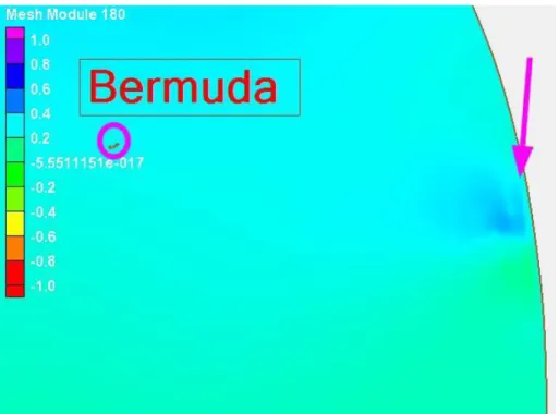
Instabilities consistently formed after a period of 20-110 days near the offshore boundary, either near the southern end (south of roughly 13 degrees latitude) or around the same latitude as Bermuda. Mesh modifications near the locations of the instabilities only delayed the formation of the instability. Modifications made attempting to prevent the instability included changing the number of nodes along and near the boundary, smoothing bathymetry, modifications to the Bay of Fundy to deal with
bathymetric issues, turning off boundary forcing of several smaller tidal harmonics, moving the boundary to -60 longitude (the location of the boundaries in the EC95 and EC2001 meshes), increasing the
horizontal eddy viscosity (ESLM) up to 50, and turning off wetting and drying and the time derivative of the advection term (NOLICAT).
Manual reviews were also carried out on the water elevation and velocity solutions at dozens of time steps for various runs, and on the boundary forcing amplitudes and phases to verify their smoothness. The only tide simulation that completed without a fatal instability and without any of the above-mentioned
modifications was a 90-day simulation with nodal factors set to 1 and equilibrium arguments set to 0. Though, this same run failed if extended to 120 days. Close inspection shows the instability east of Bermuda to be periodic, seemingly appearing at certain tide phases. The nascent instability could be seen weeks or even months before suddenly growing large and crashing the simulation, as shown in Figure 5-7.
32
Figure 5-8 and Figure 5-9 show the effects of having the advection terms turned on/off for the tidal simulation. Many improvements in amplitudes of the advection-off run are because they were done with a later version of the mesh and with an improved set of stations, i.e. station positions were changed as necessary to get them within the model domain. These changes can be seen to tighten up the model performance for several other stations (e.g. ones in the 0.5-1 m amplitude range). In both plots, the greatest deviations are found at stations in the Gulf of Maine (all stations with observed amplitudes above 1.2 m) and other areas in the northeast US. At Boston, the differences are on the order of 0.10 meters and in the northern Gulf of Maine, the differences reach 0.20 meters with the results with advection on being greater in both cases. In Long Island Sound, the sense of the deviation is reversed with M2 amplitudes being smaller for advection-on simulations. Differences between simulations with advection on and off are insignificant in the rest of the East Coast and Gulf of Mexico portions of the mesh.
Figure 5-8: Correlation of M2 constituent amplitude comparing predicted and simulated results from simulations with
33
Figure 5-9: A pseudo-geographic depiction of the effect of modification of the non-linear advection; results from simulations with non-linear advection terms turned on are plotted as blue points and off as red points.
5.3
Overall Tidal Skill
Of the 398 stations, 324 meet the target error metric of 0.2 meter root mean squared error (RMSE). Of 74 stations not meeting the target error metric, only 18 are located outside of the Gulf of Maine. The 56 points not meeting the skill metric in the Gulf of Maine owe their poor performance to the effect of disabling the advection terms in the model and to the large tide ranges characteristic of the region. The other stations exceeding the error metric are also in challenging locations, including two points located in wetlands on Florida’s west coast; six points in inland parts of Florida and Georgia; four points in secluded parts of the Chesapeake Bay; three points up the Delaware River; one point in the East River; and one point in western Long Island Sound.
The inland points in Florida and Georgia were affected by a problem endemic to the wetting and drying algorithm within ADICIRC. The problem is associated with the factors which are included in the ADCIRC solution to prevent instabilities when elements are periodically wetting and drying. Essentially under certain conditions, the model will artificially produce water over broad, slow draining areas surrounded by steep drop-offs, such as in the Georgia tidal flats. This creates an artificially high water level on the tidal flats. Additional detail regarding this issue is documented in Appendix D.
34
Figure 5-10: Geographic distribution of water level time series RMSE at 398 tide gages, highlighting points exceeding the 0.2 meter RMS error metric.
-95 -90 -85 -80 -75 -70 -65
20 25 30 35 40 45
longitude
la
ti
tu
d
e
35
6.
STORM HINDCAST VALIDATION
Surge responses during a total of ten tropical and extratropical storms were evaluated, covering a spectrum of landfalls across the US Gulf of Mexico and East coasts. The target error metric was 0.2 meters (0.66 feet) RMSE for time series data at NOAA gages as computed by the CSDL Skill
Assessment Software6. Simulated peak surges were compared to both NOAA time series data and to post-storm surveyed High Water Mark (HWM) datasets, where these datasets were available. Storms whose meteorological forcing came from a FEMA Flood Insurance Study (FIS) have model skill comparisons to those studies to give a sense of baseline performance that can be expected with the same meteorological data. However, the FEMA studies use much higher resolution meshes and (in most cases) a coupled wave model.
Model skill suffered most from differences in initial water level (model simulations were run without a starting water level anomaly adjustment) and from missing wave setup contributions. As a result, most storms’ modeled results are biased low. Some storms, particularly Ike, the 1991 Perfect Storm, and Dennis, showed poor performance for other reasons as explained in the sections below. The quality of the wind forcing was a significant factor in the overall skill of the models. For this reason, the FEMA-sourced hindcast forcing created by Ocean Weather, Inc. (OWI) was used where available because it provided the best opportunity to test the performance of the mesh. For events where OWI meteorology was not available, the model skill suffered as a result.
The CSDL Skill Assessment reported RMSE for all gages evaluated for all storms was 0.26 meters, 30% greater than the target. Modifications suggested in Section 0, specifically making some accommodation for the un-simulated mean water level effects, could bring the mean error within the target. Additional analysis and discussion are given for the individual storms in this section and for the entire set of storms as a group in Section 7.
6.1
Typical Model Setup
All storm simulations began with a 15-day tidal simulation, during which the tidal forcing was ramped up using a hyperbolic tangent ramping function for the first 10 days. Storm simulations were then hot-started from the tide ramp runs, with the duration of the storm forcing varying by storm. A separate ramping of the meteorological forcing was applied at hot-start time, which lasted 0.5 days for most storms. Following the meteorological ramping period, the simulation was completed within the actual event period, going from as little as 1.25 days up to 8 days depending on the length of the event.
All storms were modeled at their historical time by use of proper tidal harmonic phasing. The tide_fac.f7 Fortran routine was used to generate boundary and body forcing values for 13 harmonic constituents. Further details on tidal forcing are supplied in Section 5.1. All simulations were attempted with advection both on and off. Information about how this affected results is included in the sections below. Details on bottom friction, wind drag, and other spatially varying parameters are supplied in Section 4.2.
Surface forcing fields consisting of wind velocities and atmospheric pressure were provided from a variety of sources, including: 1) quality controlled high resolution wind fields created by Ocean Weather, Inc. (OWI) as part of FEMA FIS studies and provided by FEMA to NOAA for this project; 2) Hurricane Weather Research and Forecast System (HWRF) hindcasts from NOAA; 3) NOAA’s Atlantic
Oceanographic & Meteorological Laboratory (AOML) Hurricane Research Division (HRD) Surface
6 The skill assessment software provided by CSDL was modified to prevent clipping of observed surge data. By default, the software is set to remove downloaded data points more than three standard deviations from the rest of the data. This value was extended include all valid water level measurements including the surge crest.
36
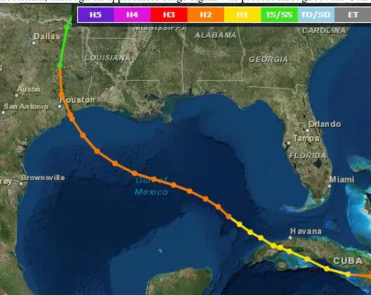
Wind Analysis System (H*Wind)8 real-time analysis fields; and 4) NHC best-track data driving the parametric hurricane vortex model included within the ADCIRC model. The storms used for hindcast analysis are shown in Table 6-1, along with an indication of the source for the wind forcings for the simulation. In the table and throughout Section 6, the storms are presented in geographic order, from west to east along the Gulf of Mexico, then south to north along the East coast, as shown in Figure 6-1.
Table 6-1: Summary of tropical and extratropical cyclone hindcast validation simulations.
Coastal Impact Area Name Year Month Wind Data Source(s)
Wind
Scaling Advection North Central Texas,
Western Louisiana. Ike 2008 Sept
OWI/FEMA Region 6:
Texas study 1.04 On
Eastern Louisiana,
Mississippi Katrina 2005 Aug
OWI/FEMA Region 4: Mississippi, Panhandle studies
1.09 On
Panhandle and
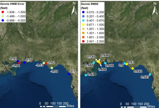
northwestern Florida. Dennis 2005 July
OWI/FEMA Region 4: Big
Bend, Panhandle studies 1.04 On Southwestern Florida Charley 2004 Oct OWI/FEMA Region 4:
Southwest Florida study 1.04 On South Carolina Hugo 1989 Sept OWI/FEMA Region 4:
South Carolina study 1.04 Off
North Carolina Floyd 1999 Sept
H*Wind; ADCIRC parametric with NHC best track (Holland)
Virginia., Washington D.C., Maryland., Delaware.
Isabel 2003 Sept OWI/FEMA Region 3:
Region 3 study 1.04 On
New England Sandy 2012 Oct HWRF 1.0 On
New England
Long Island Express or Great New England Hurricane
1938 Sept
OWI/FEMA Region 2: New Jersey/New York study
1.04 On
New England Perfect Storm or
Halloween Nor'easter 1991 Oct
OWI/FEMA Region 2: New Jersey/New York study
1.04 Off
37
Figure 6-1: Approximate landfall locations of hindcast validation events.
The majority of the simulations used OWI wind and pressure forcing obtained from FEMA studies. OWI provides 30-minute averaged marine-equivalent winds at 10 meter elevation. All storms using OWI wind forcing had their winds scaled by a factor of 1.04 (except for Hurricane Katrina), due to the differences between 10 and 30-minute wind averaging as seen in prior modeling projects and different values used in FEMA studies, including 1.00, 1.04, and 1.09. Hurricane Katrina’s OWI winds were a special case due to the way in which they were developed, which is detailed for that storm in Section 6.3. Early test
simulations for Ike, Sandy, and Floyd were made with H*Wind real-time analysis fields as they initially lacked OWI windfields, but these simulations yielded poor model skill. Alternative forcing data sources were sought for these events. HWRF fields improved the model performance for Sandy and OWI winds were eventually obtained and also improved the model skill for Ike. The only alternative source found for Floyd was the best-track + ADCIRC internal parametric wind model which did not improve the overall skill for the event.
Skill assessment for all simulations described in this section were carried out using the CSDL-developed software described in Zhang et al. (2006, 2010). Hurricane track plots shown in Figure 6-1 above and in the following sections were obtained from the NOAA Historical Hurricane Tracks tool (Office of Coastal Management9).