MARGINAL STRUCTURAL COX MODELS WITH CASE-COHORT SAMPLING
Hana Lee
A dissertation submitted to the faculty of the University of North Carolina at Chapel Hill in partial fulfillment of the requirements for the degree of Doctor of
Philosophy in the Department of Biostatistics.
Chapel Hill 2013
Approved by:
Dr. Michael G Hudgens Dr. Jianwen Cai
c ○2013 Hana Lee
ABSTRACT
HANA LEE: MARGINAL STRUCTURAL COX MODELS WITH CASE-COHORT SAMPLING
(Under the direction of Drs. Dr. Michael G Hudgens and Dr. Jianwen Cai)
A common objective of biomedical cohort studies is assessing the effect of a time-varying
treatment or exposure on a survival time. In the presence of time-varying confounders,
marginal structural models fit using inverse probability weighting can be employed to obtain
a consistent and asymptotically normal estimator of the causal effect of a time-varying
treat-ment. This document considers estimation of parameters in the semiparametric marginal
structural Cox model (MSCM) from a case-cohort study. Case-cohort sampling entails
assembling covariate histories only for cases and a random subcohort, which can be cost
effective, particularly in large cohort studies with low outcome rates. Following Cole et al.
[2012], we consider estimating the causal hazard ratio from a MSCM by maximizing a
weighted-pseudo-partial-likelihood. The estimator is shown to be consistent and
asymp-totically normal under certain regularity conditions. Computation of the estimator using
standard survival analysis software is discussed and results from a simulation study are
presented.
In the standard (associational) case-cohort Cox analysis, various methods have been
pro-posed to improve efficiency from maximum pseudolikelihood estimators of Prentice [1986a] or Self and Prentice [1988]. As the presented theory of MSCM parameter estimator is
developed based on Self and Prentice [1988] we briefly review those methods and discuss
extension of the methods to the MSCM analysis. In addition, we proposed a new method to
improve efficiency of the case-cohort MSCM analysis from a biomedical study that aims to
evaluate the causal effect of treatment on a time to event. We seek to improve the efficiency
by multiple imputation method which can make fuller use of covariate information that are
available from full cohort. The proposed method is applied to the Multicenter AIDS Cohort
Study (MACS) and the Women’s Interagency HIV Study (WIHS).
ACKNOWLEDGMENTS
I would like to express my deepest appreciation to my advisor, Dr. Michael G.
Hudgens who arouse my passion toward research and taught me how joyful research is.
Working with him was certainly the best thing ever happened to me at Chapel Hill. I
can hardly imagine my dissertation without his endless support and insightful guidance. I
sincerely thank him for everything. I dare to say that he is the best advisor in the universe.
My second deepest appreciation goes to my co-advisor Dr. Jianwen Cai. She is my role
model as a female biostatistician in academia. I started dreaming of working in academia
while working with her. She has the substance of genius, and is full of responsibility. My
dissertation is indebted to her brilliance. Someday, I also want to be a great role model for
peers and students.
Without my advisors, this dissertation would not have been completed. They have
guided me to the right path whenever I lost a direction. During the past two years, they
were like parents holding their childs hands and teaching how to walk. Like a toddler, I
had fears and pains for the first few steps. However, every step with my advisors eventually
became my priceless properties. I will never forget the moments walking together.
I would like to thank my wonderful committee members, Drs. Stephen R. Cole, Danyu
Lin, and Donglin Zeng as well. I cannot imagine any better committee members. Dr. Cole’s
brilliant idea initiated my dissertation and his support with the Multicenter AIDS Cohort
and the Women’s Interagency HIV studies dataset completed my dissertation. Besides his
expertise in research, he is also a warmhearted person who was very supportive to my
dissertation. Dr. Lin’s comments and suggestions brought invaluable developments to my
first paper. After my preliminary exam, Dr. Zeng provided me a brilliant idea which was
further developed into my last project. I am very grateful to these committee members for
spending their time regardless of their very busy schedule.
I am also thankful to my dear friends who shared both painful and joyful moments with
always with me in my heart.
Last but not least, I dedicate my thesis to my love of life, Wonyul Lee.
TABLE OF CONTENTS
LIST OF TABLES . . . viii
1 Introduction . . . 1
2 Literature Review . . . 4
2.1 Cox Models . . . 4
2.2 Causal Inference and Marginal Structural Cox Models . . . 7
2.2.1 Causal Inference and Potential Outcomes . . . 8
2.2.2 Marginal Structural Cox Models . . . 11
2.3 Cox Models with Case-cohort Sampling . . . 14
2.4 Statistical Methods to Improve Efficiency . . . 16
3 Marginal Structural Cox Models with Case-cohort Sampling . . . 19
3.1 Introduction . . . 19
3.2 Marginal Structural Cox Model Estimators . . . 21
3.2.1 Notation, Assumptions, and Model . . . 21
3.2.2 Inverse Probability Weights . . . 24
3.2.3 Weighted-Psuedo-Partial-Likelihood . . . 26
3.3 Consistency . . . 28
3.4 Asymptotic Normality . . . 37
3.5 Implementation and Simulation . . . 47
3.5.1 Implementation . . . 47
3.5.2 Simulation . . . 50
3.6 Supplemental Material . . . 52
4 Efficient Inference of Case-Cohort Marginal Structural Cox Models . . 62
4.1 Introduction . . . 62
4.2 General Methods for MSCM Case-Cohort Estimators . . . 65
4.3 Improving Efficiency of the Estimation . . . 68
4.3.2 Imputation Method . . . 70
4.4 Results . . . 75
4.4.1 Simulation Studies . . . 75
4.4.2 Real Data Analysis . . . 78
4.5 Discussion . . . 84
5 Summary and Future Research . . . 86
BIBLIOGRAPHY . . . 87
LIST OF TABLES
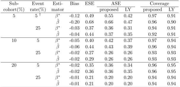
3.1 Summary of simulation study . . . 51
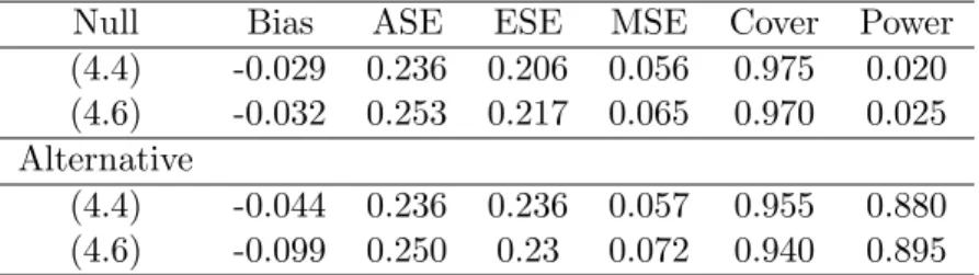
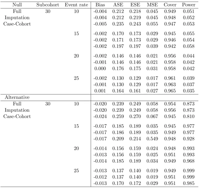
4.1 Simulation studies to compare performance of estimators . . . 77
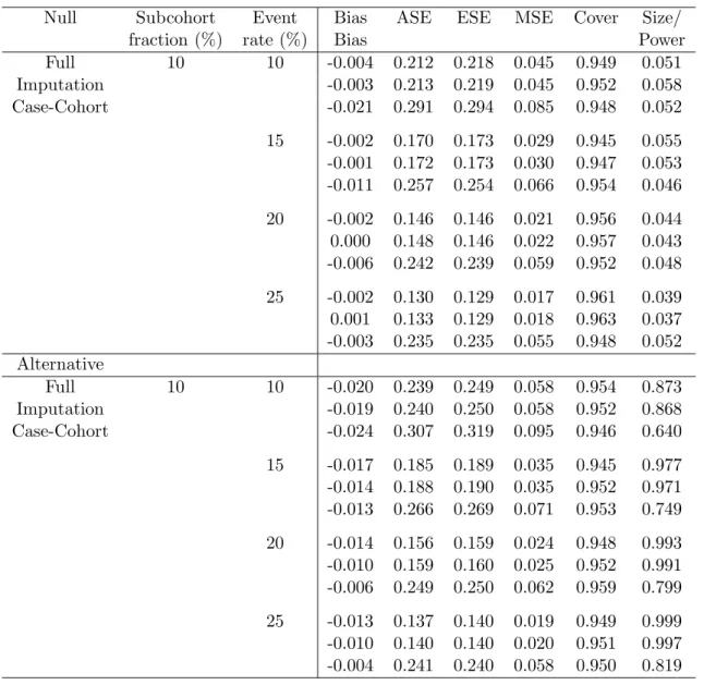
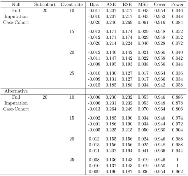
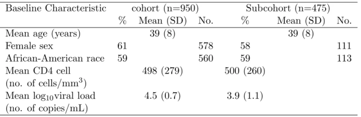
4.2 Simulation studies to compare performance of estimators whenα=.1 . . . . 79 4.3 Simulation studies to compare performance of estimators whenα=.2 . . . . 80 4.4 Simulation studies to compare performance of estimators whenα=.3 . . . . 81 4.5 Baseline characteristics of the full and the 50% subcohort subjects . . . 83
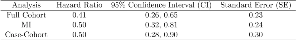
4.6 Full cohort, 20% subcohort with MI, and case-cohort MSCM analyses . . . . 83
Chapter 1
Introduction
Biomedical cohort studies are often conducted with the goal of assessing the effect of a
time-varying treatment (or exposure) on a survival time. In such studies there may exist
time-dependent covariates which are simultaneously (i) confounders and (ii) affected by
prior treatment on the causal pathway from treatment to disease. In the presence of
time-varying confounders affected by prior treatment, standard methods such as Cox regression
modeling with time-varying covariates do not in general yield consistent estimators of the
causal effect of treatment [Robins, 1986, 1998; Robins and Rotnitzky, 1992; Hern´an,
Brum-back and Robins, 2001]. On the other hand, marginal structural models (MSMs) fit using
inverse probability weighting can be employed to obtain consistent estimators of the causal
effect of a time-varying treatment on an outcome of interest, even if there are time-varying
confounders affected by prior treatment [Robins, 1999].
For example, consider the Multicenter AIDS Cohort Study (MACS), an observational
study of HIV-positive homosexual men. Using data from MACS, Hern´an, Brumback and
Robins [2001] showed that (i) current CD4 count and Pneumocystis carinii pneumonia (PCP) status were independent risk factors for death and were predictive of subsequent
treatment with zidovudine (AZT) and prophylaxis therapy (i.e., confounders), and (ii)
pro-phylaxis therapy was a protective risk factor for the development of PCP subsequently.
Thus, to assess the effect of AZT and prophylaxis therapy on mortality in MACS, a method
is required that can appropriately account for time-varying confounders affected by prior
treatment (in particular, PCP status). Applying standard (i.e., unweighted) Cox
regres-sion with time-dependent covariates to the MACS data, Hern´an, Brumback and Robins
nonusers, suggesting that treatment increases the risk of death in HIV-positive
homosex-ual men, contrary to results from randomized clinical trials. On the other hand, fitting
a marginal structural Cox model (MSCM) with inverse probability weighting yielded an
estimated hazard ratio for AZT of 0.67 (95% CI 0.46, 0.98), in agreement with results from
randomized trials of AZT. The difference in hazard ratio estimates between the unweighted
Cox regression model and the MCSM with inverse probability weighting is not surprising
given the aforementioned established results about the (in)consistency of these estimators
in the presence of time-varying confounders affected by prior treatment.
Recently, Cole et al. [2012] considered fitting MSCMs via inverse probability weighting
in the presence of case-cohort sampling. The case-cohort study design is a cost-efficient
approach to estimate treatment effects in large cohorts with low event rates, when treatment
or covariate information is expensive. The design entails randomly selecting a subcohort
from the entire cohort. Covariate information is then collected only from the random
subcohort and from individuals that are observed to experience an event (i.e., cases), saving
cost and effort relative to obtaining covariate information from the full cohort. In addition to
being cost efficient, the case-cohort design enjoys other benefits. For instance, the subcohort
can serve as a basis for real time covariate monitoring during the course of the study.
Also, because the subcohort is chosen randomly, survival times to different diseases can be
analyzed using the same subcohort [Self and Prentice, 1988].
In the presence of case-cohort sampling, Cole et al. [2012] considered estimating the
causal hazard ratio of a MSCM via inverse probability weighting. Simulation studies
indi-cated the estimator proposed by Cole et al. [2012] can perform well empirically, however no
formal justification for their estimator has been developed to date. Therefore, following Cole
et al. [2012], we consider estimating the causal hazard ratio of a MSCM via inverse
probabil-ity weighting in case-cohort studies and establish consistency and asymptotic normalprobabil-ity for
the estimator that maximizes a weighted-pseudo-partial-likelihood (WPPL) under certain
regularity conditions.
The approach utilized in this proposal entails standard counting process and martingale
theory. Using this formulation readily enables practical implementation of the methods
using existing survival analysis software. Framing the problem using counting processes
studies or in the presence of competing risks. In the special situation that the subcohort
equals the full cohort, the proposed inverse probability weighted estimator is asymptotically
equivalent to the estimator in Robins [1999]. Moreover, in this case our proof gives an
alternative consistency and normality proof to Robins [1999], who did not utilize the usual
counting process framework.
The outline of the remainder of this document is as follows. Chapter 2 begins with an
introduction to methods for survival analysis primarily focusing on Cox models. A review
of case-cohort studies is next. Then we introduce MSCMs on the basis of causal inference
and potential outcome framework. This Chapter concludes with a review of some statistical
methods devised to improve efficiency in the standard Cox regression analysis with
case-cohort sampling. In Chapter 3 the estimator of the hazard ratio of a MSCM in the presence
of case-cohort sampling is introduced, and proofs of consistency of the parameter estimators
under the full and the case-cohort settings are shown. Also, we establish full distributional
theories of the parameter estimators under the full cohort and the case-cohort settings
in the same Chapter. How to implement a MSCM using existing software such as R or
SAS is described in Chapter 3.5, along with the simulation study results. Details to show
asymptotic distributional theory of the case-cohort MSCM parameter estimate are provided
in 3.6. In Chapter 4 we propose a new method that can improve efficiency in the
case-cohort MSCM analysis. We start from a review of general methods for MSCM case-case-cohort
estimators, including our proposed methods introduced in Chapter 3, and demonstrate
why the discussed methods devised to improve efficiency in the standard case-cohort Cox
regression analysis may not be applicable to the causal setting. We propose a new method
which aim to utilize all subject in the estimation and show numerical study results. The
proposed method is applied to a real observational HIV study data composed of two data
sets, the Multicenter AIDS Cohort Study and the Women’s Interagency HIV Study.
Chapter 2
Literature Review
2.1 Cox Models
Here, we assume a study consists ofnunique individuals who are indexed byi=1, ..., n. Let Ti denote failure (or survival) time of a subject i in a study, where T = 0 represents
the time of initiation of follow-up and τ represents study end point. We essentially as-sume that the failure time is on continuous basis. Let Ci denote the time of censoring
and Xi =min(Ti, Ci) denote the observed time from the subject i. δ(Xi) =I{Ti < Ci} is
an event indicator where I{⋅} is an usual indicator function. In addition, let p×1 vector of Zi(Xi) = (Z1i(Xi), ..., Zpi(Xi)) denote time-dependent covariates information collected
from the subjecti. Throughout we assume (Xi, δi, Zi)(i=1, ..., n) ben independent
repli-cates of(T, δ, Z)thatZ is bounded. Also, letNi(t)be a stochastic process which denote the
number of failures of subjectiby timet. We use the notationdNi(t)to indicate the number
of events of the subjectioccurred in[t, t+dt) for sufficiently smalldt. Since failures occur in continuous time, we only allow jumps of size 1 and no simultaneous jumps can occur in
[t, t+dt) for the process Ni(t). LetYi(t)=I{Ti ≥t, Ci ≥t} denote whether an individual
is still alive and being able to be observed (to fail) at timet, having a left-continuous sam-ple paths. This process is called “at risk” process. Then the data for the ith participant
(Xi, δi, Zi) can be rewritten as{Ni(u), Yi(u), Zi(u)∶0≤u≤t}.
In biomedical studies, we are often interested in identifying/quantifying risk (or
prognos-tic) factors related to response. Cox regression models, including Cox proportional hazards
models, introduced by Cox [1972] are the most commonly used approach to explore (or
denote the hazard (or risk) of being failed associated with Z(t), i.e.,
λ(t∣Z(t))= lim
dt→0Pr(t≤T ≤t+dt∣T≥t, Z(t))/dt.
Then Cox models are given by
λ(t∣Z(t))=λ0(t)exp{β′0Z(t)} (2.1)
whereλ0(t∣Z(t))is an unknown baseline hazard and β0=(β0,1, ..., β0,p)is a set of unknown
regression parameters. λ0(⋅)describing how the hazard changes over time at baseline levels of covariates, i.e., Z(t)=0 for allt≥0. β0 describes the effect of covariates on the hazard changes over time. Under this model, we can compare two hazards under different covariate
levels (e.g., treated or untreated) in the logarithm scale. For instance, consider two
obser-vations iand i∗ that differ in their covariate values at time tby Z(t)and Z∗ respectively. Then the hazard ratio for two observations is
exp{β0Z′ (t))}/exp{β0Z′ ∗(t)}=exp{β0′(Z(t)−Z∗(t))},
and therefore the log of the hazard ratioβ0′(Z(t)−Z∗(t))can be explained by the parameter
β0. When Z(t) ≡Z for all t≥0 then this models are also referred to as the proportional hazards models since the hazard ratio at any timetis independent of timet. Explicitly, the hazard ratio for two observationsiand i∗ in the above example is
exp{β0Z′ }/exp{β0Z′ ∗}=exp{β0′(Z−Z
∗)}
which is constant over time t.
λ0(⋅) is an unknown function and parametric distributional assumptions such as uni-form, exponential, weibull on λ0(⋅) is available. Other than distributional assumption, a monotonic or step function assumption can also be made. However, Cox [1975] proposes a
partial likelihood approach which enables to estimate the parameter of interest β0 in (2.1) while the λ0(⋅) remains unspecified. Consistent estimator for β0 can be obtained by using the partial likelihood score function
U(β)=
n
∑
i=1
δi{Zi(Xi)−
S(1)(β0, Xi)
S(0)(β, X
i)}
(2.2)
where S(k)(β, Xi) = n−
1 ∑n
i=1Yi(Xi)Zi⊗k(Xi)exp{β′Z(Xi)} for k = 0,1,2 under standard
independent censoring assumption. Here, we definea⊗0≡1,a⊗1 ≡a, and a⊗2=a′awhich is defined by thep×pmatrix with(i, j)th elementaiaj forp×1 vectorsa. The maximum
par-tial likelihood estimator ˆβ, defined as the solution to the score equationU(βˆ)=0, is shown to converge in distribution to Normal with mean zero and a covariance matrix which can
consistently be estimated by−{∂U(β)/∂β∣β=βˆ}− 1
based on martingale formulation
(Ander-sen and Gill [1982]). Using an integral repre(Ander-sentation, log-likelihood function corresponding
to (2.2) can be written by
l(β)=
n
∑
i=1∫
τ
0 β
′Z
i(u)−log[ n
∑
l=1
Yl(u)exp{β′Zl(u)}]dNi(u). (2.3)
The theory and application of the Cox models almost always assumes an exponential
form for the relative risk function on regression variables, however, other regression forms
such as a linear relative risk function (e.g., 1+β′0Z) are more natural to use in some applications. Prentice and Self [1983] addresses that a linear relative risk regression model
may provide a more convenient framework for studying epidemiologic risk factor interactions
than an exponential relative risk regression. Using the same counting process formulation of
Andersen and Gill [1982] but with some more stability and regularity assumptions, Prentice
and Self [1983] establishes asymptotic distribution theory for a class of intensity function
regression models in which the usual exponential regression form is relaxed. In Prentice
and Self [1983], (2.1) is extended by
λ(t∣Z(t))=λ0(t)r{β′0Z(t)} (2.4)
and (2.3) is modified by
l(β)=
n
∑
i=1∫
τ
0 β
′Z
i(u)−log[ n
∑
l=1
where r{⋅} is a generalized relative risk function, which is an arbitrary non-negative twice differentiable function assumed to be locally bounded away from zero in some
neighbor-hood of β0. Estimators obtained by solving ∂l(β)/∂β = 0 is shown to be consistent and asymptotically normal, based on asymptotic normality of the score function along with
con-sistency of the observed information matrix −n∂2l(β)/∂β2. Some stability and regularity conditions, beyond those of Andersen and Gill [1982], are required to show the consistency
of the observed information matrix.
2.2 Causal Inference and Marginal Structural Cox Models
The purpose of this chapter is to review causal inference on the basis of potential outcome
framework, relevant notation and assumptions, and finally to review the MSCMs. Before
we start reviewing what the causal inference is, we address that under what circumstances
standard statistical methods may fail to provide causal inference.
The term time-varying confounder is commonly used for time-varying risk factors of an outcome of interest that also predicts the subsequent exposure (or treatment).
Post-treatment variables potentially affected by Post-treatment and also affecting the response are
referred to asintermediate variables. Unlike randomized clinical trials, many observational studies with long-term follow-up period often incorporate time-dependent covariates which
are simultaneously confounders and intermediate variables on the causal pathway from
exposure to disease. As a result, it may not be possible to obtain causal interpretation
from the parameter estimator obtained using standard statistical methods. It is also true
when the time-to-event response is considered. Standard methods of using the ordinary
Cox models (2.1) or (2.4) adjusting for the time-dependent covariates may fail to provide
appropriate causal effect of the exposure on an outcome of interest.
In the presence of such time-varying confounders, marginal structural models (MSMs,
Robins [1999]), or marginal structural Cox models when the failure time is of interest,
are powerful tools for assessing causal effects of time-varying treatments on an outcome of
interest. MSMs are used increasingly to provide semi-parametric estimates of total (Bodnar
et al. [2004]), joint (Robins, Hern´an and Brumback [2000]; Hern´an, Brumback and Robins
[2000]), and direct/indirect (VanderWeele [2009b]) causal effects of exposures on an outcome
in epidemiologic studies.
In following sections, we give introduction to causal inference with relevant concepts,
notation, and assumptions to understand MSMs as tools to draw causal inference. Hereafter
we assume an observational study wherein confounding effect exists, which interested in
evaluating treatment effect on a participant’s failure time such as HIV studies for example.
2.2.1 Causal Inference and Potential Outcomes
Most causal inferences are based on the idea of potential outcomes under all possible
treatment assignments, introduced by Neyman [1923]. The potential outcomes, which
in-clude observed and unobserved outcomes, are sometimes called counterfactual outcomes
(or simply counterfactuals) since these outcomes could have happened contrary to what we
actually observed. In this framework, causal inference can be considered as a missing data
problem letting the potential outcomes as missing data, especially the unobserved outcomes
to be the missing outcomes.
Below we modify some of the notation introduced from earlier section to be more suitable
to a hypothetical biomedical study and to the causal inference framework. Capital letters
represents random variables and lower case letters represents values of the random variables
or constants, the same as before. Now, letAi(t)be the treatment vector of subjectiwhere
tdenotes the time since the beginning of the subject’s follow-up. LetLi(t) denote a vector
of assembled covariates such as CD4 counts and PCP level from subject iat time t. The subscript iwill sometimes be suppressed in our notation since we assume Ai(t) and Li(t)
are random vectors for each subject drawn independently from a distribution common to
all subjects. Let V represent baseline covariates which can be a part of L(0). A(t) and
L(t) are defined to be zero when t<0. Note that a p×1 covariate vector Z(t) introduced from earlier section equals to {A(t), L(t)}.
Potential (Counterfactual) Outcomes In the context of causal inference, overbars
are used to represent history up to and including time tsuch that A(t)={A(u); 0≤u≤t}
and L(t) is defined analogously, assuming that decisions related to treatment at tis made after obtaining the covariate information att, i.e.,L(t)is temporally earlier thanA(t). Let
given C.
a represents each possible treatment plan; a= {a(t) ∶ 0≤ t ≤τ} where τ is the study end point, same as before. Each possible value of a can be interpreted as a pre-specified treatment plan. Practical examples of a might be never treated (i.e., a(t) = 0 for all
t ∈ [0, τ]), treated starting at a pre-specified time t1 (i.e., a(t) =I[t > t1]), treated from baseline (i.e.,a(t)=1 for allt∈[0, τ]), etc. ThenTarepresents a random variable implying
a subject’s potential failure time had (possibly contrary to what we observe from actual
study) the subject been treated with historya. For example, one can use notationT0(t)to represent a subject’s potential failure time if he had treated from baseline,Tt1(t) if he had treated since time t1>0, and T∞ if he had never treated. At each time-to-event t such as death or disease occurrence time, a set of three different failure times (T0(t), Tt1(t), T∞(t)) comprises potential outcomes.
Assumptions Most causal models that are based on the idea of potential outcomes rely
on the following four assumptions.
1. Consistency In reality, we only observe the outcome T with a subject’s actual treatment history A, i.e., T = Ta=A = TA. This identity is called the fundamental
“consistency” assumption that links the potential failure times Ta to the observed
data(TA, A).
2. No unmeasured confounders There are no unmeasured confounders for the effect of
A(t) on T if, for alla,
Ta⊥⊥A(t)∣A(t−), L(t) (2.6)
holds (Robins [1999] and Hern´an, Brumback and Robins [2000]).
3. Positivity We say that positivity assumption holds if Pr[A(t)=a∣L(t)=l] >0 for all a∈{0,1} andl such that Pr[L(t)=l]≠0.
4. No misspecification of the model As we always assume that the model we employ is a correct model to analyze data, a causal model to estimate the effect of treatment
is assumed to be correctly specified.
Informally, consistency means that the outcome for every treated individual equals to the
subject’s outcome if he/she had received treatment, and the outcome for every untreated
individual equals to his/her outcome had the subject remained untreated. No unmeasured
confounders means that the risk of failure under the potential treatment history a among the treatment group equals to the risk under the same potential treatment history among
untreated group for each a. Therefore the treated and untreated groups are exchangeable as in a randomized trial. For this reason, the assumption is also called “exchangeability”
or “sequential randomized assumption” in some articles since it implies that potential
out-comes are exchangeable regardless of treatment history given all relevant confounder history
as if in a randomized trial. However, if there exists any unmeasured confounder that
pre-dicts A(t) at time t then the potential outcomes are no longer independent of treatment history. Positivity simply means that the conditional probability of receiving every value of
treatment is greater than zero. No missspecification of the model assumption is the natural
assumption to make any statistical inference and may be tested using sensitivity analysis.
In general, the no unmeasured confounders assumption is a crucial assumption to draw
causal inference using some causal models but is not statistically testable. A more complete
studies on these condition and causal inference can be traced back to Rubin [1974], Rubin
[1976], Rubin [1980], Robins [1986], Greenland and Robins [1986], and Robins [1987].
Causal and Statistical Exogeneity Informally, a treatment process is referred to be
a “causally exogenous” process if the conditional probability of receiving a treatmentA(t)
given past treatment and (measured and unmeasured) prognostic factor history depends
only on past history of treatment historyA(t−). Mathematical definition of causal exogene-ity may vary across different articles. Definitions of presented in this proposal are adopted
from Hern´an, Brumback and Robins [2001]. The article defines a treatment process to be
“causally exogenous” if
Ta⊥⊥A(t)∣A(t−) (2.7)
for all treatment plansa, which is equivalent to state that Ta is independent ofA(t). Also,
which is given by
L(t)⊥⊥A(t)∣A(t−). (2.8)
This implies that conditioning on treatment history before timet, probability of receiving treatment at timetdoes not depend on the history of measured time-dependent prognostic factors up to t. It can be seen that (2.8) is a necessary condition for A(t) to be causally exogenous, but (2.8) does not imply (2.7) due to the possibility of unmeasured confounders.
Following Robins et al. [1992], Hern´an, Brumback and Robins [2001] also defined that there
are no unmeasured confounders for the effect of A(t) on T if, for alla,
Ta⊥⊥A(t)∣A(t−), L(t) (2.9)
holds.
Robins [1999] showed that statistical exogeneity implies causal exogeneity under the
assumption of (2.9). Also it is well recognized that treatment parameters of a correctly
specified association model have causal interpretation if the treatment process is causally
exogenous. Therefore, causal inference can be drawn from using standard association models
if condition (2.8) is true assuming that (2.9) holds.
2.2.2 Marginal Structural Cox Models
Robins [1999] introduced MSMs combined with inverse-probability-treatment-weights
(IPTW) as a method to draw causal inference in the presence of confounding, which rely
on the potential outcome framework. IPTW can be considered a type of inverse sampling
weights to account for missing data or sampling bias problem. By weighting observations via
IPTW, we can reflect back the balanced design from observational data having confounding
effect (under the assumptions described from Chapter 2.2.1).
We first review IPTW and then describe MSCMs after.
Inverse-Probability-Treatment-Weighting Suppose that we can correctly model the
probability of receiving treatment at time tgiven past treatment history and covariate his-tory, i.e., Pr[A(t)∣A(t−), L(t)]. Then we could measure the degree of statistical exogeneity
of the treatment process through time tby calculating a following weight at t:
WT(t)=∏
k≤t
Pr[A(k)∣A(k−)]
Pr[A(k)∣A(k−), L(k)], (2.10)
which is referred to as inverse-probability-of-treatment-weights (IPTW). Under the four assumptions of consistency, no unmeasured confounders, positivity, and no misspecification
of the model to estimate the weights, we can create a hypothetical population by weighting
each subject at risk at each failure time with (2.10). This hypothetical or weighted study
population is known as the pseudo-population. Robins [1999] and Lemma A.1 of Hern´an, Brumback and Robins [2001] proved that L(t) no longer predicts A(t) in each pseudo-population created at each failure timet (note that (2.10) equals to 1 at any timet if L(t)
does not predictA(t)∣A(k−), i.e., the treatment process is statistically exogenous). Then it follows that the treatment process is causally exogenous in the pseudo-population under the
assumption of no unmeasured confounders. Thereby one can employ standard association
models to estimate the treatment effect which can further be interpreted as a causal effect.
As the same manner, we can effectively adjust bias occurred by censoring due to loss to
follow-up when time-to-event data is considered. This can be done by considering
inverse-probability-of-censoring-weights (IPCW), sayWC, where
WC(t)=∏
k≤t
Pr[C(k)=0∣C(k−)=0, A(k−)]
Pr[C(k)=0∣C(k−)=0, A(k−), L(k)], (2.11)
under the assumptions of independent censoring and no unmeasured confounders for
cen-soring. Here, C(k)=0 means a subject remains uncensored prior to time k and C(k)=1 means censored at that time.
Robins [1997] first introduced IPTW, which is called unstablized weights, as a tool to adjust non-ancillary treatment process in the observational study, however, it has a slightly
different form than (2.10). Stablized weights has the same denominator as in (2.10) but the
Besides this, truncated (Cole and Hern´an [2008]) and normalized (Xiao, Abrahamowicz and
Moodie [2010]) weights are also introduced and these weights can be considered as types of
stablized weighs as they all aim to adjust variability of IPTW and make it stable over time.
Stablized weights are generally recommended to employ in practice as they lead to, often
remarkably, more efficient estimators of causal treatment effect.
When survival data is considered, inverse-probability-weights (IPW) defined by W(t)≡
WT(t)×WC(t) are the stabilized weights. For estimation of random weights W(t) see Hern´an, Brumback and Robins [2000], Hern´an, Brumback and Robins [2001], and Cole and
Hern´an [2008]. Since investigators should assume that the model to estimate IPW (e.g., a
logistic model), sensitivity analysis results with different model specifications will help to
see validity of the correct model assumption in practice.
Marginal Structural Cox Models Marginal Structural Cox Models (MSCMs) are
given by
λTa(t)=λ0(t)exp{β
′
0f(a(t))} (2.12)
where λTa(t) is the hazard of failure at time t if all subjects in a study population had followed treatment history a through time t, λ0(⋅) is an unspecified baseline hazard func-tion corresponding to the hazard if all subject had been untreated, and β0 is an unknown parameter vector. If we are interested in current treatment effect of zidovudine on AIDS
so that f(a(t)) in (4.1) becomes a(t), and exp(β0) has a causal interpretation such as the ratio of the hazard of getting AIDS at any time t if all subjects had been continuously exposed to zidovudine compared with the hazard rate at t had all subjects remained un-exposed. This model is a causal model for the marginal distribution of the variables Ta
which is the potential outcomes that are generally unobserved. Hence estimation of the
causal log rate ratio β0 cannot be made directly through this model. In the absence of confounding, association implies causation thereby we can use the standard Cox regression
model to obtain causal estimates. As mentioned the above, Robins [1999] showed that we
can create a psuedo-population via IPW at each failure time t in which time-dependent prognostic factors no longer predict treatment history. Robins [1999] also proved that the
causal relationship between treatment and hazard in the psuedo-population is the same as
in the original study population, and the estimator of treatment effect obtained by using
the standard Cox regression model based on the psuedo-population converges in probability
to β0 in (4.1). Therefore the estimator of treatment effect obtained by using the ordinary time-dependent Cox model adjusting (only) for the treatment, after weighting each
individ-ual at each failure time by IPW, can have causal interpretation as it converges in probability
to β in (4.1).
2.3 Cox Models with Case-cohort Sampling
The case-cohort study proposed by Prentice [1986a] and Self and Prentice [1988] is a cost-effective design particularly when large epidemiologic cohort studies with rare disease or
infrequent event such as HIV studies are considered. This design involves random selection
of a subcohort (or a stratified random sample) from the entire cohort and all participants
who experience the event of interest, henceforth cases. By monitoring covariate information
only for a random subcohort and for all cases we can gain cost and effort saving. The
subcohort constitutes the comparison set of cases occurring at a range of failure times as
well as a basis for covariate monitoring during the course of cohort follow-up (Self and
Prentice [1988]).
Prentice [1986a] considers Cox modeling on time-to-response case-cohort data. Suppose that a random subcohort ˜C of size ˜nis selected from the entire cohortC of size n. Then the log partial likelihood is modified by
l∗(β)=
n
∑
i=1∫
τ
0 β
′Z
i(u)−log[ ∑ l∈C∪{i}˜
Yl(u)r{β′Zl(u)}]dNi(u). (2.13)
in the presence of case-cohort sampling, which is termed a logpseudolikelihood by Prentice [1986a].
Self and Prentice [1988] provides a full range of asymptotic theory for parameter
estima-tors of the Cox models in the presence of the case-cohort sampling using a slightly different
log partial likelihood form
˜
l(β)=
n
∑
i=1∫
τ
0 β
′Z
i(u)−log[∑ l∈C˜
Estimators obtained by solving ∂˜l(β)/∂β = 0 are shown to converge in probability to β0
and asymptotically normally distributed via same techniques as in Andersen and Gill [1982]
and Prentice and Self [1983], i.e., by showing asymptotic normality of the score function
along with consistency of the observed information matrix. It is also shown that estimators
obtained by solving ∂l∗(β)/∂β = 0 and ∂˜l(β)/∂β =0 converge in probability to the same quantity, β0, in Self and Prentice [1988].
Several other authors such as Binder [1992] and Lin and Ying [1993] expand the idea
of the case-cohort design and provide estimating equations to obtain estimators in more
general settings. Binder [1992] describes how to create a family of survey-related sampling
plans, and provided a procedure for fitting the proportional hazards models to survey data
with complex sampling designs including the case-control sampling. Estimating equation
proposed in the article is an extension of the standard score function equation in (2.2), with
incorporating probability of being sampled. In particular, Binder [1992] proposes a score
function given by
U∗(β)=
n
∑
i=1
wiδi{Zi(Xi)−
S∗(1)
(β0, Xi)
S∗(0)(β, X
i) }
,
where now the statistics were modified by
S∗(r)(β, Xi)=n−
1 n ∑
i=1
wiYi(Xi)Zi⊗k(Xi)exp{β′Z(Xi)}
fork=0,1,2, andwi is the inclusion probability for the subject i, i.e., wi=1/πi if the
sub-ject i is selected in the sample and 0 otherwise. Estimators obtained by solving U(β)=0 are then shown to be asymptotically normally distributed. Lin and Ying [1993] provides a
general solution to the problem of missing covariate data under the Cox models, considering
case-cohort data as a possible example of missing covariate data. The estimating function
proposed in the article is an approximation to the partial likelihood score function with
full covariate measurements, which reduces to the score function of Self and Prentice [1988]
in the special setting of the case-cohort designs. The approximate partial likelihood score
function is given by
˜
U(β)=
n
∑
i=1
δiHi(Xi){Zi(Xi)−
˜
S(1)(β0, Xi)
˜
S(0)(β, X
i) }
where Hi is a p×p diagonal matrix with indicator functions {H1i(⋅), ..., Hpi(⋅)} as the
diagonal element with H1i(Xi) being an indicator whether Zji(Xi) is available at failure
time Xi, ˜S(k)(β, Xi) are defined by n−1∑ni=1H0i(Xi)Yi(Xi)Zi⊗k(Xi)exp{β′Z(Xi)} fork=
0,1,2 withH1i(Xi)being an indicatorI{Hji(Xi)=1}for allj=1, ..., p. Then approximate
partial likelihood estimators (APLE) are the root to the estimating equation ˜U(β)=0. The resulting parameter estimators are consistent and asymptotically normal with a covariance
matrix for which a simple and consistent estimator is provided. Also, the asymptotic theory
of the APLE are established on regularity conditions that are much simpler to interpret and
check than those in Self and Prentice [1988].
Despite the efficiency of the sampling methods, applications of the case-cohort designs
had been limited because of perceived analytic complexity, especially on the variance
com-putation proposed from Self and Prentice [1988]. Self and Prentice [1988] variance estimator
is not easy to implement as it includes computation of covariances between score
contri-butions from pairs of different risk sets. Simple robust variance estimators are proposed
by Lin and Ying [1993] and Barlow [1994] as a solution to the computational challenges
in variance computation, and also practical implementation of the Cox models to the real
case-cohort data is addressed by Therneau and Li [1999] and Barlow et al. [1999]. Therneau
and Li [1999] describes how to obtain Self and Prentice [1988], Barlow [1994], and Lin and
Ying [1993] parameter estimators along with their variance estimators using standard
soft-ware packages, with SAS and S-Plus as particular examples. Barlow et al. [1999] illustrates
weighting methods as model fitting techniques and provides a SAS macro that computes
the weighted estimates and the robust covariance matrix.
2.4 Statistical Methods to Improve Efficiency
In the standard associational case-cohort Cox analysis, various methods have been
seek to improve efficiency of the hazard ratio estimation compared to Prentice [1986a] and Self and Prentice [1988].
Unweighted Psuedo-Partial Likelihood Estimators As described in 2.3, Prentice
[1986a] proposed a pseudo-likelihood approach for the hazard ratio parameter estimation in the Cox model along with heuristic procedures for parameter estimation when the
case-cohort design is applied. Asymptotic distribution theory of the case-case-cohort maximum
pseudo-likelihood estimator was developed by Self and Prentice [1988] using martingale
technique and finite population convergence results. Both Prentice [1986a] and Self and Prentice [1988] do not accommodate case sampling or stratified sampling of controls, i.e.,
they considered unweighted pseudo-likelihoods.
Unweighted Psuedo-Partial Likelihood Estimators After Prentice [1986a] and Self and Prentice [1988], various methods have been proposed as means of improving the
efficiency of the hazard ratio estimation (compared to Prentice [1986a] and Self and Pren-tice [1988]) in the standard (associational) case-cohort Cox regression analysis. Chen and
Lo [1999] studied a different class of estimating equations than Prentice [1986a] and Self and Prentice [1988] by constructing different risk sets in the estimating equations. They
proposed to utilize complete information of all cases when calculating ratio of weighted
av-erages based on risk set information inside the estimating equations. In particular, authors
proposed three different estimating equations which all use the empirical distribution of
covariate Z among cases to the conditional joint distributions of(Z, X) among cases, but use different estimators of p=pr{δ(Xi)=1}. Chen et al. [2001] found an optimal sample
reuse method via local averaging, and proposed a unified weighted estimating equation,
that can be used in various sampling design, to improve efficiency.
Time-Varying Inverse-Sampling-Weights Barlow [1994] and Barlow et al. [1999]
con-sidered estimators based on weighted pseudo-likelihood estimation. At each failure time,
contribution of cases and nonfailures (controls) at risk are weighted by either fixed or
time-varying inverse-sampling-weights (ISW) to account for subcohort sampling.
Using All Available Covariate Data from Full Fohort Later, methods that seek
to utilize some of the phase 1 covariate information were proposed. Borgan et al. [2000]
considered a stratified sampling by a phase 1 variable which is a correlate of exposure,
to incorporate statum-specific ISW in the estimating equation. Stratum-specific ISW can
be calculated using empirical sampling fraction within each stratum. He proposed three
different estimating equations by considering different types of weights. Simulation studies
suggested that the stratified estimator II with time-varying ISW, referred to as BII estimator
from herein, is the most efficient among the existing estimators. Kulich and Lin [2004]
established asymptotic theory for the BII type of estimators. In addition they developed a
class of weighted estimators which utilize all available covariate information from the full
cohort data. Proposed weighted estimators are 1) doubly weighted (DW) estimator and 2)
combined doubly weighted (CDW) estimator which involve general time-varying ISW. The
methods involve a modeling step for prediction of the values of each partially missing phase 2
variables, and is likely of greatest use when there are only 1 or 2 such variables. The authors
suggest to use CDW estimator in practice as DW estimator is efficient only if a model to
predict the phase 2 variables given all the phase 1 variables is correct. Numerical studies
indicated that the CDW estimator is more efficient then other existing estimators such as
Chen and Lo [1999], Borgan et al. [2000], and Chen et al. [2001]. The efficiency gain for the
phase 2 covariates depends on the ability of the first-phase data to predict the true values
of the partially missing variables. Later, Breslow et al. [2009a] and Breslow et al. [2009b] considered calibration or estimation of ISW by making use of phase 1 covariate information.
Calibration method adjusts ISW to be as close as possible to the sampling weights subject
to a certain constraint. Estimation methods uses ISW as inverse of inclusion probabilities
estimated from a logistic regression model that predicts which cohort subjects are sampled
at phase 2. Simulation study and real data analysis reported by Breslow et al. [2009b] showed that such adjustment on ISW can dramatically improve precision of the baseline
hazard ratios, which are estimated for baseline covariates, i.e., a part of phase 1 variables.
They also showed that the methods can improve precision for the phase 2 covariates when
their values may be imputed with reasonable accuracy for the non-subcohort controls.
In Chapter 4 we demonstrate how we can extend some of the aforementioned methods
might be extended to the causal setting and discuss why some of the methods might not be
Chapter 3
Marginal Structural Cox Models with Case-cohort Sampling
3.1 Introduction
Biomedical cohort studies are often conducted with the goal of assessing the effect of a
time-varying treatment (or exposure) on a survival time. In such studies there may exist
time-dependent covariates which are simultaneously (i) confounders and (ii) affected by
prior treatment. In the presence of time-varying confounders affected by prior treatment,
standard methods such as Cox regression modeling with time-varying covariates do not in
general yield consistent estimators of the causal effect of treatment Robins [1986, 1998];
Robins and Rotnitzky [1992]; Hern´an, Brumback and Robins [2001]. On the other hand,
marginal structural models (MSM) fit using inverse probability weighting can be employed
to obtain consistent estimators of the causal effect of a time-varying treatment on an
out-come of interest, even if there are time-varying confounders affected by prior treatment
Robins [1999].
For example, consider the Multicenter AIDS Cohort Study (MACS), an observational
study of HIV-positive homosexual men. Using data from MACS, Hern´an, Brumback and
Robins [2001] showed that (i) current CD4 count and Pneumocystis carinii pneumonia (PCP) status were independent risk factors for death and were predictive of subsequent
treatment with zidovudine (AZT) and prophylaxis therapy, and (ii) prophylaxis therapy
was a protective risk factor for the development of PCP subsequently. Thus, to assess
the effect of AZT and prophylaxis therapy on mortality in MACS, a method is required
that can appropriately account for time-varying confounders affected by prior treatment (in
particular, PCP status). Applying standard (i.e., unweighted) Cox regression with
estimated hazard ratio of 1.85 (95% CI 1.49, 2.30) for AZT users versus nonusers, suggesting
that treatment increases the risk of death in HIV-positive homosexual men, contrary to
results from randomized clinical trials. On the other hand, fitting a marginal structural
Cox model (MSCM) with inverse probability weighting yielded an estimated hazard ratio
for AZT of 0.67 (95% CI 0.46, 0.98), in agreement with results from randomized trials of
AZT. The difference in hazard ratio estimates between the unweighted Cox regression model
and the MSCM with inverse probability weighting is not surprising given the aforementioned
established results about the (in)consistency of the standard estimators in the presence of
time-varying confounders affected by prior treatment.
Recently, Cole et al. [2012] considered fitting MSCMs via inverse probability weighting
in the presence of case-cohort sampling. The case-cohort study design is a cost-efficient
approach to estimate treatment effects in large cohorts with low event rates, when treatment
or covariate information is expensive. The design entails randomly selecting a subcohort
from the entire cohort. Covariate information is then collected only from the random
subcohort and from individuals that are observed to experience an event (i.e., cases), saving
cost and effort relative to obtaining covariate information from the full cohort. In addition to
being cost efficient, the case-cohort design enjoys other benefits. For instance, the subcohort
can serve as a basis for real time covariate monitoring during the course of the study.
Also, because the subcohort is chosen randomly, survival times to different diseases can be
analyzed using the same subcohort Self and Prentice [1988].
In the presence of case-cohort sampling, Cole et al. [2012] considered estimating the
causal hazard ratio of a MSCM via inverse probability weighting. Simulation studies
indi-cated the estimator proposed by Cole et al. [2012] can perform well empirically, however no
formal justification for their estimator has been developed to date. Therefore, following Cole
et al. [2012], we consider estimating the causal hazard ratio of a MSCM via inverse
probabil-ity weighting in case-cohort studies and establish consistency and asymptotic normalprobabil-ity for
the estimator that maximizes a weighted-pseudo-partial-likelihood (WPPL) under certain
regularity conditions.
The approach utilized in this paper entails standard counting process and martingale
theory. This formulation readily enables practical implementation of the methods using
be helpful in future work, e.g., in fitting MSCMs to data from nested case-control studies or
in the presence of competing risks. In the special situation that the subcohort equals the full
cohort, the proposed inverse probability weighted estimator is asymptotically equivalent to
the estimator in Robins [1999]. In this case our proof gives an alternative consistency and
normality proof to Robins [1999], who did not utilize the usual counting process framework.
We also derive a new variance estimator that arises from the counting process formulation
under both full and case-cohort settings. Empirical results presented in this paper indicate
that in certain scenarios the proposed variance estimator may be preferred to the so-called
“robust” variance estimator Lin and Ying [1993] employed in Cole et al. [2012].
The outline of the remainder of this paper is as follows. In §3.2, estimators of the hazard ratio of a MSCM in the presence of case-cohort sampling are introduced, including
the estimator proposed by Cole et al. [2012]. Consistency and asymptotic normality are
established in §3.3 and §3.4, respectively. §3.5 explains how one can directly obtain the proposed inverse probability weighted estimators using standard survival analysis software,
and presents a simulation study.
3.2 Marginal Structural Cox Model Estimators
3.2.1 Notation, Assumptions, and Model
Capital letters will represent random variables and lower case letters will represent values
of the random variables or constants. Consider an observational cohort study where the
outcome of interest is a survival time T, based on the time from study entry until some particular outcome occurs. Throughout we assume T is continuous so that there are no tied failure times between individuals. During the course of the study individuals may
dropout or discontinue participation in the study, such that T is not observed but rather right censored at the last time the individual was under study. Suppose individuals may
or may not elect to receive treatment at various points of time during the study. LetAi(t)
indicate whether subjectiis on treatment at timet. If more than one treatment is available, thenAi(t) is a vector of treatment indicator variables corresponding to the joint treatment
levels. In the sequel we assumeAi(t) is ap×1 vector and treatment variation is irrelevant
VanderWeele [2009a]. The subscriptiwill often be suppressed, when there is no ambiguity,
because we assume random vectors are drawn independently from a distribution common
to all subjects. Let L(t) denote a vector of covariates, such as CD4 count or PCP status, at timet. LetL(0) represent baseline covariates. Overbars are used to represent history up to and including time tsuch thatA(t)={A(u)∶0≤u≤t}and L(t) is defined analogously. Assume that decisions related to treatment at t are made after obtaining the covariate information at t, i.e., L(t) is temporally prior to A(t). For a case-cohort study, the time varying covariates L(t) and treatment A(t) are by design observed only for the cases and individuals in the random subcohort (while under study);L(t)andA(t)are missing for all other individuals. Corresponding to the subcohort, let ˜C denote the set of indices of size
˜
n≤nthat are randomly selected without replacement from the set{1, . . . , n}corresponding to the entire cohort.
Let adenote a possible (static) treatment plan, i.e., a={a(t)∶0≤t≤τ}whereτ is the study duration. Assume τ =1 hereafter without loss of generality. Each possible value of
a can be interpreted as a prespecified treatment plan. Assuming a single treatment (i.e.,
p =1), practical examples of a might be never treat (i.e., a(t) =0 for all t∈ [0,1]), treat starting at a prespecified timet1<1 (i.e., a(t)=I{t≥t1}where I{⋅} is the usual indicator function), treat from baseline (i.e.,a(t)=1 for allt∈[0,1]), etc. DefineTato be a subject’s
potential failure time had (possibly contrary to what was observed in the actual study) the
subject been treated according to a. Let ⊥⊥ denote statistical independence; e.g., A⊥⊥B∣C
denotesA is independent of B given C. Assume
T =Ta ∀asuch thata(t)=A(t) ∀t≤T, (3.1)
Ta⊥⊥A(t)∣A(t−), L(t) ∀a, (3.2)
pr[A(t)∣A(t−), L(t)]>0 ∀t∈[0,1] such that pr[A(t−), L(t)]>0 (3.3)
which are referred to as the causal consistency, conditional exchangeability, and positivity
assumptions, respectively. Assumption (3.1) states that, in the absence of censoring, the
observed failure timeT equals the potential failure timeTafor all treatment plansa
states that the conditional probability of receiving any particular treatment is greater than
zero. Of these three assumptions, only (3.3) can be tested empirically. Sensitivity analysis
may be useful in assessing the robustness of inference drawn to violations of assumption
(3.2) Robins, Rotnitzky and D [1999].
Consider the MSCM
λTa(t)=λ0(t)exp{β
′
0f(a(t))}
where λTa(t) is the hazard of failure at time t if all individuals in the population had followed treatment plana through timet,λ0(t) is an unspecified baseline hazard function corresponding to the hazard if all individuals had been untreated through time t, f(a(t))
is a specified function of treatment history up to timet, and β0 is an unknown parameter vector. Hereafter, we consider the MSCM
λTa(t)=λ0(t)r{β
′
0a(t)} (3.4)
where for notational convenience we let r{⋅}=exp{⋅}. For example, if we are interested in the causal effect of current AZT treatment on mortality of HIV-positive homosexual men,
then r(β0) is the ratio of the hazard of death at time t had all subjects in the population alive at timetbeen exposed to AZT compared to had the subjects been unexposed at time
t. Note (3.4) focuses on the effect of current treatment status only; however, the results presented below are valid for any specified f(a(t)).
In this paper the counting process framework is employed to study the large sample
behavior of estimators of β0. Note that all processes discussed hereafter refer to observed processes. Let (Ω,F,P) be a complete probability space and let {Ft ∶ t ∈ [0,1]} be an
increasing right-continuous family of sub σ-algebras of F consisting of failure times, co-variates and treatment histories up to time t, and censoring histories up to time t+ for all subjects in a cohort of size n. That is, the filtration with respect to the probability space is the same as the usual filtration, except that treatment histories are now separated
from covariate histories. Let Ni(⋅) be a counting process adapted to Ft representing the
number of failures of subjectiby timetsuch that dNi(t)indicates the number of events of
subjecti that occurred in [t, t+dt) for sufficiently small dt. Because failures are assumed to occur in continuous time, we only allow jumps of size 1 and no simultaneous jumps can
occur in[t, t+dt). LetCi(t)=0 indicate that subjecti remained uncensored prior to time
t and Ci(t) = 1 otherwise. The treatment process Ai(⋅) and the censoring process Ci(⋅)
are assumed to be piece-wise constant point processes with cadlag (right-continuous with
left-hand limits) step-function sample paths. The processes A(⋅) and C(⋅) are assumed to have jumps that can occur at no more than a finite number of time points. Informally, this
means that all participants follow (approximately) the same visit schedule. This
assump-tion should be reasonable in studies with regularly scheduled follow-up visits (e.g., every six
months) and good study compliance. We refer to censoring as ignorable (or noninformative)
if the cause-specific hazard of being censored attamong subjects alive and uncensored does not depend on the failure timesTagiven prior treatment/covariate historyA(t−)andL(t−)
(Hern´an, Brumback and Robins [2001]). Let Yi(t) =I{Ni(t)=Ci(t) =0} denote whether
an individual is at-risk of being observed to fail at time t, having left-continuous sample paths, and assume pr[Y(1)>0]>0.
3.2.2 Inverse Probability Weights
Suppose that we can correctly model the probability of receiving treatment at time t
given the past treatment history and covariate history. Then we can consistently estimate
the following weights
WT(t)=∏
k≤t
pr[A(k)∣A(k−)]
pr[A(k)∣A(k−), L(k)], (3.5)
which will be referred to as inverse-probability-of-treatment-weights (IPTWs). Note that we
can consistently estimate the numerator probabilities in (4.2) based on sample proportions
because A(⋅) is assumed to have at most a finite number of jumps over the study period. Under (3.2) to (3.3), in the absence of censoring, Robins [1999] showed that a consistent
estimator of the unknown parameterβ0 in (3.4) can be obtained by fitting an ordinary time-dependent Cox model with the contribution of subject ito the risk set at time tweighted by estimates of (4.2). Informally we can think of the analysis via IPTWs as reweighting the
the measured confoundersL, from a population where L(t)⊥⊥A(t)∣A(t−) holds at time t. The weighted study population is sometimes called apseudo-population.
Dropout (i.e., right censoring) may introduce selection bias if dropout is associated with
exposure and dropout is associated with the outcome. In the presence of such censoring, we
still can obtain a consistent estimator ofβ0 by fitting the ordinary Cox model but weighting a subject alive and uncensored at timet by estimates ofWT(t)×WC(t), where
WC(t)=∏
k≤t
pr[C(k)=0∣C(k−)=0, A(k−)]
pr[C(k)=0∣C(k−)=0, A(k−), L(k)], (3.6)
under the assumption of no unmeasured confounders for censoring, an analogous
assump-tion to (3.3) for censoring, and assuming that we can correctly model the denominator
probabilities in (3.6) Robins [1999]. Here the weighted study population can be thought
of as a pseudo-population in which there is no confounding due to measured covariates
or selection bias due to censoring. In §3.2.3, we will make use of the (stabilized) weights defined by W(t)≡WT(t)×WC(t) after modifying (4.2) by addingC(k)=0 to the condi-tioning events in both the numerator and the denominator Hern´an, Brumback and Robins
[2000]. HereafterW(t)will be referred to as inverse-probability-weights (IPWs). Note that (4.2) and (3.6) are finite products. In addition, (3.3) ensures non-zero probabilities in the
denominators of (4.2) and (3.6) and hence the IPWs at all tare bounded.
Results presented in this article are not limited to a specific form of the weights W(t). The proposed methods are applicable to different inverse probability weighting analysis
provided that the IPWs (or IPTWs in the absence of censoring) are bounded, such as when
truncated [Cole and Hern´an, 2008] and normalized [Xiao, Abrahamowicz and Moodie, 2010]
weights are employed. Under the assumption of finite support of the treatment and
censor-ing processes, unstabilized weights [Hern´an, Brumback and Robins, 2001] are also bounded.
However, unstabilized weights are known to be highly variable and are by design
mono-tone increasing functions of t. Other weights such as stabilized, truncated, and normalized weights are generally recommended in practice as they lead to more efficient estimators of
the causal treatment effect.
We now briefly describe estimation of the random weights W(t), denoted by ˆW(t). One may specify a pooled logistic model (treating each person-visit as an observation) to
estimate the probability in denominators of (4.2) and (3.6) at each time (for example, at
each visit), then plug in the estimated probabilities to (4.2) and (3.6) Hern´an, Brumback
and Robins [2000, 2001]. We assume throughout that the model to estimate denominator
probabilities in the IPWs is correctly specified. In practice, investigators may want to
explore the sensitivity of the regression coefficients to different model specifications for
estimating the weights.
3.2.3 Weighted-Psuedo-Partial-Likelihood
In this section we consider two weighted-pseudo-partial-likelihoods (WPPLs) which form
the basis for obtaining consistent estimators of β0 in the presence of case-cohort sampling. The WPPLs are formed by weighting individual contributions to the usual partial likelihoods
by Wi(t) assuming that Wi(t) is known. In the case-cohort setting, we consider a set of
individuals ˜C of size ˜n≤n that is randomly selected without replacement from the entire cohort {1, . . . , n}.
The log-WPPL created by individual-time-specific weights at timetunder the full cohort setting is given by
l(β, t;W)= (3.7)
n
∑
i=1∫
t
0 Wi(u)[β
′A
i(u)−log n
∑
l=1
Wl(u)Yl(u)r{β′Al(u)}]dNi(u),
which is motivated by the weighted estimating equations proposed by Robins [1993].
The log-WPPL in the case-cohort setting is
˜
l(β, t;W)= (3.8)
n
∑
i=1∫
t
0 Wi(u)[β
′A
i(u)−log∑ l∈C˜
Wl(u)Yl(u)r{β′Al(u)}]dNi(u).
Note (3.8) is slightly different from the log-WPPL proposed by Cole et al. [2012], which is
l∗(β, t;W)= (3.9)
n
∑
i=1∫
t
0 Wi(u)[β
′A
i(u)−log ∑ l∈C∪{i}˜
The log-WPPLs (3.8) and (3.9) differ only in whether a case outside the subcohort ˜C contributes to the risk set. In the absence of weights, i.e., Wi(u)=1 for alli and u, (3.8)
reduces to the log-likelihood considered by Self and Prentice [1988] and (3.9) reduces to the
log-likelihood considered by Prentice [1986b]. Estimators that maximize (3.8) or (3.9) will be shown to converge in probability to β0.
Note that under (3.1) each (observed) counting processNi(⋅)(i=1, ..., n)can be uniquely
decomposed into the sum of its intensity processλi and a local square integrable martingale
Mi, i.e.,
Ni(t)=∫ t
0
λi(u)du+Mi(t), t∈[0,1], (3.10)
where the intensity process is given by
λi(t)=Yi(t)r{β0A′ i(t)}λ0(t), (3.11)
which embodies the same parameters as in (3.4).
Define ˆβ, ˜β, and β∗ to be solutions to ∂l(β,1; ˆW)/∂β = 0, ∂˜l(β,1; ˆW)/∂β = 0, and
∂l∗(β,1; ˆW)/∂β=0, respectively. Consider the following processes
X(β, t;W)=n−1{l(β, t;W)−l(β0, t;W)} (3.12)
=n−1
n
∑
i=1∫
t
0 Wi(u)[(β−β0)
′A i(u)
−log∑
n
l=1Wl(u)Yl(u)r{β′Al(u)}
∑n
l=1Wl(u)Yl(u)r{β0′Al(u)}]
dNi(u),
˜
X(β, t;W)=n−1{˜l(β, t;W)−˜l(β0, t;W)} (3.13)
=n−1∑
i∈C∫ t
0
Wi(u)[(β−β0)′Ai(u)
−log∑l∈C˜Wl(u)Yl(u)r{β
′A l(u)}
∑l∈C˜Wl(u)Yl(u)r{β
′
0Al(u)}]
dNi(u)
corresponding to (3.7) and (3.8) respectively. We will first show thatX(β, t; ˆW)and (3.12) are asymptotically equivalent, and so are ˜X(β, t; ˆW) and (3.13). Thus, further technical developments will be made based on (3.12) and (3.13). We then show that (3.12) and
(3.13) at t= 1 converge in probability to functions of β which are concave with a unique
maximum β0 under certain conditions. Using the same argument as in Andersen and Gill [1982], it follows that ˆβ →p β0 and ˜β →p β0. That β∗ →pβ0 can be shown analogously by
usingX∗(β, t;W)=n−1
{l∗(β, t;W)−l∗(β0, t;W)}. Asymptotic normality of ˆβ and ˜β will be shown via asymptotic normality of score statistics corresponding to (3.7) and (3.8).
3.3 Consistency
For a p×1 column vector c, let c⊗0 =1, c⊗1 =c, and c⊗2 =cc′, ci denote i-th element
of c, and cij denote (i, j) element of c⊗2. Norms are defined by ∣∣c⊗2∣∣ =supi,j∣cij∣, ∣∣c∣∣ =
supi∣ci∣, and ∣c∣ = (∑c2i)
1/2
= (c′c)1/2. Also let r(0){β′A(t)} = r{β′A(t)}, r(1){β′A(t)} =
A(t)r{β′A(t)}, andr(2){β′A(t)}=A(t)⊗2r{β′A(t)}.
CONDITIONS.
A (Uniform consistency of estimated weights)
sup
i∈{1,...,n}
t∈[0,1]
∣Wˆi(t)−Wi(t)∣≡MWˆ →p 0.
Along with the assumption of no misspecification of the model used to estimate
denom-inator probabilities in W(⋅), the finite number of jumps assumption on the treatment and censoring processes are sufficient for this condition to hold. From a practical point of view,
having a finite number of time points when treatment status can change or when censoring
might occur may be reasonable to assume in many settings. For instance, studies often
have planned visits at finite discrete intervals when a patient may have treatment altered.
Similarly, the censoring time for a subject is often assumed to be the last observed visit
time before the subject became lost-to-follow-up.
B (Stability of weights) Individual time-specific weights Wi(t) and the corresponding
es-timators ˆWi(t) are strictly positive and bounded, i.e., there exist positive real numbers
M1 andM2 such that
sup
i∈{1,...,n}
t∈[0,1]
Wi(t)≤M1, and sup i∈{1,...,n}
t∈[0,1]
ˆ
Note that ˆW(⋅) and W(⋅) are assumed to be predictable with respect to the filtration
Ftbecause weights are determined by predictable processes: A(⋅),L(⋅), and their histories.
All weights discussed in §3.2.2 satisfy the conditions A and B under any circumstances, except the unstabilized weights. Unstabilized weights satisfy conditions A and B under the
assumption of finite support ofA(⋅) and C(⋅).
C (Finite interval) ∫01λ0(t)dt<∞
D (Asymptotic stability)
(i) There exists a neighborhood B0 of β0 and functions s( 0)
, s(1), and s(2) defined on
B0×[0,1] such that
sup
β∈B0
t∈[0,1]
∣∣S(j)(β, t)−s(j)(β, t)∣∣→p0, j=0,1,2
where S(j)(β, t) = n−1∑ni=1Yi(t)r(j){β′Ai(t)} for j = 0,1,2, which are the same
quantities as given in Andersen and Gill [1982] with covariatesZi(t)being replaced
by the treatment process Ai(t).
(ii) Let SW(j) (k) = n
−1 ∑n
i=1Wi(t)kYi(t)r(j){β′Ai(t)} for j = 0,1,2 and k = 1,2. There
exists a neighborhoodBofβ0,B⊆B0, and functionss(j)W
(k)defined onB×[0,1]such
that
sup
β∈B
t∈[0,1] ∣∣SW(j)
(k)(β, t)−s
(j)
W(k)(β, t)∣∣→p0, j=0,1,2;k=1,2
(iii) SW(0)
(1)(β0, t) converges in distribution to a mean zero Gaussian random variable uniformly in t, i.e.,
n1/2{SW(0)
(1)(β0, t)−s
(0)
W(1)(β0, t)}→dN(0, σ 2
(t)), uniformly int∈[0,1],
for someσ2 (t).