5357.pdf

(1)

STATISTICAL ANALYSIS OF FINANCIAL TIME SERIES AND

RISK MANAGEMENT

by Hongyu Ru

A dissertation submitted to the faculty of the University of North Carolina at Chapel Hill in partial fulfillment of the requirements for the degree of Doctor of Philosophy in the Department of Statistics and Operatiaons Research (Statistics).

Chapel Hill 2012

Approved by:

Eric Ghysels

Chuanshu Ji

Amarjit Budhiraja

Shankar Bhamidi

(2)

c

2012

Hongyu Ru

(3)

Abstract

HONGYU RU: STATISTICAL ANALYSIS OF FINANCIAL TIME SERIES AND RISK MANAGEMENT.

(Under the direction of Eric Ghysels.)

The dissertation studies the dynamic of volatility, skewness, and value at risk for financial returns. It contains three topics.

The first one is the asymptotic properties of the conditional skewness model for asset pricing. We start with a simple consumption-based asset pricing model, and make a connection between the asset pricing model and the regularity conditions for a quantile regression. We prove that the quantile regression estimators are asymptotically consistent and normally distributed under certain assumptions for the asset pricing model.

The second one is about dynamic quantile models for risk management. We propose a financial risk model based on dynamic quantile regressions, which allows us to estimate conditional volatility and skewness jointly. We compare this approach with ARCH-type models by simulation. We also propose a density fitting approach by matching conditional quantiles and parametric densities to obtain the conditional distributions of returns.

(4)

Acknowledgments

Being a graduate student, there is nothing else more exciting than writing the acknowledgement in my dissertation, as it is one of the best opportunities for me to extend my heartfelt gratitude and deepest appreciation to all who make this possible over the years.

First of all, I would like to thank my dissertation advisor Professor Eric Ghysels for his extraordinary support and encouragement. His unparalleled enthusiasm, dedication and vision on research always give me inspiration to keep going on my work.

I would also like to sincerely thank Professor Chuanshu Ji who also supervised my research. It has been a hard journey for me to pursue this degree. Whenever I was in trouble, he has always tried his best to help me out on both research and life throughout the years.

Moreover, I am very grateful to other member of my dissertation committee: Pro-fessor Amarjit Budhiraja, ProPro-fessor Riccardo Colacito, ProPro-fessor Shankar Bhamidi and Professor Eric Renault for their fruitful discussions and stimulations that led me to finish this dissertation.

(5)

List of Figures

2.1 HYBRID quantile regression and MIDAS quantile regression . . . 50

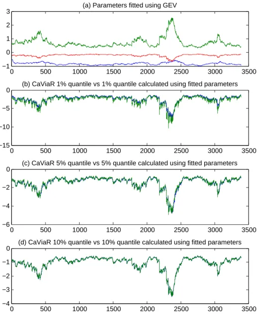
2.2 Comparison of quantiles by quantile distribution fits and CAViaR model 51

2.3 Comparison of Expected Shortfall(ES) by quantile distribution fits and

regression based ES of CAViaR quantiles . . . 52

3.1 Conditional Moments of xt for multiple horizons: moments ofxt+1|xt in

blue, xt+3|xt in green and xt+12|xt in red . . . 68

3.2 Conditional Moments of excess return for multiple horizons: moments

(8)

List of Tables

2.1 Hybrid quantiles and MIDAS quantiles for 5% VaR . . . 43

2.2 Hybrid quantiles and MIDAS quantiles for 1% VaR . . . 44

2.3 Summary of Model Specifications . . . 45

2.4 Summary of Parameters in Simulation Study . . . 46

2.5 Comparison of σt using QLIKE . . . 47

2.6 Comparison of σt using MSEprop . . . 48

2.7 Comparison of VaR using MSE . . . 49

3.1 Monthly Calibration . . . 62

3.2 Distribution of Predictive Components for Monthly Calibration . . . . 62

3.3 Equity return for γ = 15 . . . 63

3.4 Equity return for γ = 10 . . . 64

3.5 Multihorizon equity return for γ = 15 . . . 65

3.6 Multihorizon equity return for γ = 15 . . . 66

(9)

Chapter 1 Asymptotic Properties of Quantile-based Conditional

Skewness Models for Asset Pricing

1.1 Introduction

It has been documented by empirical studies that the distribution of stock market returns, either conditional or unconditional, can not be fully characterized by just mean and variance. Many previous studies have shown that the stock market returns are negatively skewed(see e.g. Harvey and Siddique (2000)). Researchers begin to incorporate the third moment - skewness, into financial models and applications. One of the applications of using skewness is portfolio selection. Harvey and Siddique (2000) has discussed about investors’ preference on the skewness of a portfolio. A portfolio with positive skewness is preferred by investors if everything else is equal. But all those results are subjected to the robustness of the measure of skewness due to the following reasons.

(10)

(2004)). Kim and White (2004) has surveyed several more robust measures of skewness based on quantiles and moments, which have been originally introduced by statisti-cians(see, e.g. Bowley (1920)). But those are only unconditional skewness measures. To study the dynamics of the stock market returns or financial time series, we need a robust measure for conditional skewness.

(11)

regression model that can be used forn-period, long-horizon return based on daily infor-mation. They find that conditional skewness still varies across time even for GARCH-and TARCH-filtered returns. In this chapter, we focus on the quantile regression models of Ghysels, Plazzi, and Valkanov (2010a).

The asypototic properties of those conditional quantile models have been studied by several papers(see, e.g., White, Kim, and Manganelli (2008), Engle and Manganelli (2004)). They show that the conditional quantile estimators are consistent and asymp-totically normal under some regulation conditions. But those regulation conditions are hard to be verified empirically. Motivated by the limitation of those regularity condi-tions, we are seeking from modeling the data generating process(DGP) from an asset pricing model to derive the regularity conditions of the quantile regression model of Ghysels, Plazzi, and Valkanov (2010a). In other words, we want to construct the link between those regulation conditions proposed by White, Kim, and Manganelli (2008), and Engle and Manganelli (2004) and basic DGPs with some simple assumptions.

(12)

Tsionas (2003) has extended Burnside (1998) to allow for any shock that has moment generating functions. Both of them have analytical solution for price-dividend ratio,

and therefore returns. Tsionas (2003) can generate conditional skewness,1 _{but we don’t}

know if it can create time-varying conditional skewness. Bekaert and Engstrom (2010) may be another option, which has both analytical solutions and allows for time-varying

conditional skewness for consumption growth.2

In this paper, we start with a rather conventional asset pricing framework based on discounted dividend streams. Initially we use closed-form formulas of Burnside (1998) and Tsionas (2003) using first a Gaussian setting and subsequently a general setting that allows us to characterize DGP’s for which we subsequently study the asymptotic properties of conditional quantile regressions and skewness measures. We have proved that the conditional quantile estimators are consistent and asymptotically normalunder those simple assumptions for the DGP of asset pricing we use.

This chapter is structured as follows. Section 1.2 describes the asset pricing model. Section 1.3 describes the quantile regression model. In Section 1.4, we explore the asympototic properties of quantile regression under the assumed data generating pro-cess. Section 1.5 concludes this chapter and describes the future works. Regulation conditions and proofs are in Section 1.6.

1.2 The Asset Pricing Model

First order condition of asset pricing to price an asset that entitles a dividend Dt

in each period satisfy

Pt=Et[St,t+1(Pt+1+Dt+1)],

1_{For example, if the shock distribution is a general Edgeworth expansion, then it allows for skewness.}

2_{But we don’t know if we can prove all the regularity conditions under this model, since they}

(13)

where Pt is price of the asset at time t, St,t+1 is stochastic discount factor(SDF). We consider a representative agent with CRRA preference and denote the price-dividend

ratio asvt=Pt/Dt, then we have

vt=Et

" β

Ct+1

Ct

−γ

(1 +vt+1)

Dt+1

Dt

#

, (1.1)

where γ is the coefficient of relative risk aversion, β is the discount factor, and Ct is

the consumption at time t. Assume the log dividend growth xt = log(Ct+1/Ct) =

log(Dt+1/Dt) follows AR(1) process

xt= (1−ρ)µ+ρxt−1+ξt, (1.2)

whereρ is the persistent parameter, and ξt is an i.i.d sequence of random variables.

Assumption 1 (i) |ρ|<1 and ρ6= 0;

(ii) Let Mξt(s) ≡ Eexp(sξt) be the moment generating function(MGF) of ξt, Mξt(s)

exists;

(iii) Let fξt(ξt) be the probability density of ξt, fξt(ξt) is everywhere continuous,

con-tinuously differentiable and fξt(ξt)>0.

The unconditional distribution of xt is µ+ (1−ρ)

−1

ξt and MGF of xt is Mxt(s) =

exp(µs)Mξt(s/(1−ρ)). Tsionas (2003) shows that

vt=

∞ X

i=1

βiexp [ai+bi(xt−µ)]≡

∞ X

i=1

zi, (1.3)

whereα ≡1−γ, θ ≡(1−γ)/(1−ρ)

ai =αiµ+ i

X

j=1

logMξt(θ(1−ρ

(14)

bi =α

ρ

1−ρ(1−ρ

i

).

The conditions for stationary and bounded equilibrium to exist are given by Tsionas (2003).

Assumption 2 Let r ≡βexp (αµ)Mξt(θ), r <1.

Lemma 1 Under Assumption 1, 2,

(i) the series vt converges;

(ii) the series vt have finite moments of every integer order.

Proof: See Tsionas (2003).

We are now in position to study the property of the returns generated from this asset pricing model. The log return can be expressed as

rt+1 = log

Pt+1+Dt+1

Pt

= log(1 +vt+1)−logvt+xt+1. (1.4)

Lemma 2 E|rt|3 <∞ if Assumption 1, and Lemma 1 holds.

Proof: See Section 1.6.

Given Assumption 1 and 2, it is possible to show that the series of returns have finite moments of every integer order. Here we just show that the series of returns have finite third moments, which is sufficient for our latter use. The proofs for the returns to have higher order moments are similar.

1.3 The Empirical Quantile Model

(15)

A robust measure of conditional asymmetry

In section 1.2, the returns generated from the DGP’s are one-period return, which can be daily, weekly, or monthly, etc. We are interested in the asymmetry in the

conditional distributions of n-period returns. Let rt,n =

Pn−1

j=0rt+j, for n ≥ 2, be the

log continuously compounded n-period return of an asset, wherertis the one-period log

return. Let Fn(r) =P (rt,n< r) be the unconditional cumulative distribution function

(CDF) of rt,n, and Fn,t|t−1(r) = P(rt,n < r|It−1) be the conditional CDF given the

information setIt−1. Theθth quantile can be defined as

q∗_θ

k(rt,t+n)≡inf{r:Fn(r) = θk}, θk ∈(0,1].

IfFn(r) and Fn,t|t−1(r) are strictly increasing, then the θth quantile of return rt,n is

qθ(rt,n) =Fn−1(r), θ∈(0,1]

and the conditional θth quantile of return rn,t is

qθ,t(rn,t) =F_n,t−1|t−1(r), θ ∈(0,1]. (1.5)

For the sake of simplicity, we could assume that Fn(r) and Fn,t|t−1(r) are strictly

increasing such that the inverse of Fn(r) or Fn,t|t−1(r) is unique. Later in the next

section, we are going to show that strictly increasing can be verified under standard regularity conditions.

(16)

Bowley’s (1920) robust coefficient of skewness is defined as

CA(rt,n) =

(q0.75(rt,n)−q0.50(rt,n))−(q0.50(rt,n)−q0.25(rt,n))

q0.75(rt,n)−q0.25(rt,n)

(1.6)

where q0.25(rt,n), q0.50(rt,n) and q0.75(rt,n) are the 25th, 50th, and 75th unconditional

quantiles of rt,n.

Groeneveld and Meeden (1984) have proposed four properties that any reasonable

skewness measure should satisfy. That is for skewness measure γ(yt) (See Kim and

White (2004)):

(i) for any a >0 and b, γ(yt) =γ(ayt+b);

(ii) if yt is symmetric, then γ(yt) = 0;

(iii) −γ(yt) =γ(−yt);

(iv) if F and G are cumulative distribution function of yt and xt, and F <c G, then

γ(yt)≤γ(xt), where <c is a skewness-ordering among distribtutions.

The measure (1.6) satisfies all the four conditions (See Groeneveld and Meeden (1984)). Also this measure is normalized to be unit independent with values between

−1 and 1. The negative(positive) values of this measure indicate skewness to the

left(right). Although this measure is robust, it is an unconditional skewness measure, which can not be used to study the dynamics of conditional asymmetry and those properties of financial time series.

Recently, White, Kim, and Manganelli (2008) and Ghysels, Plazzi, and Valkanov

(2010a) have used a conditional version of (1.6) given information It−1, which makes

(17)

They define

CAt(rt,n) =

(q0.75,t(rt,n)−q0.50,t(rt,n))−(q0.50,t(rt,n)−q0.25,t(rt,n))

q0.75,t(rt,n)−q0.25,t(rt,n)

. (1.7)

where q0.25,t(rt,n), q0.50,t(rt,n) and q0.75,t(rt,n) are the 25th, 50th, and 75th conditional

quantiles ofrt,n. To estimate (1.7), we need estimate the conditional quantiles ofrt,n. In

the next section, we present our models and estimation methods for those conditional quantiles in (1.7).

Conditional quantile specification and estimation

We denote the θth conditional quantile of rt,n at time t as qθ,t(rt,n;δθ,n), where

δθ,n is the vector of parameters to be estimated for θth quantile at horizon n. Denote

the information set that contains the daily information up to time t −1 as It−1 =

{xt−1, xt−2, ...}, where xt is a vector of daily conditioning variables. We use a mixed

data sampling (MIDAS) approach to setup the model for conditional quantile of rt,n,

which are multiple horizon returns, based on daily returns in the information set It−1.

In other words, we use daily returns as regressors. The model is defined as follows

qθ,t(rt,n;δθ,n) =αθ,n+βθ,nZt(κθ,n) (1.8)

Zt(κθ,n) = D

X

d=1

wd(κθ,n)xt−d (1.9)

whereδθ,n = (αθ,n, βθ,n, κθ,n)

0

are unknown parameters to estimate. Following Ghysels,

Santa-Clara, and Valkanov (2006), we specify ωd(κθ,n) as

ωd(κθ,n) =

f(d−_D1/2, κ1,θ,n, κ2,θ,n)

PD

m=1f(

m−1/2

D , κ1,θ,n, κ2,θ,n)

(18)

where κθ,n = (κ1,θ,n, κ2,θ,n) is a 2-dimensional row vector that reduces the number of

weights for lag coefficient to estimate fromDto 2,f(z, a, b) =za−1(1−z)b−1/β(a, b),

β(a, b) = Γ(a)Γ(b)/Γ(a+b), and Γ is Gamma function. We specify the daily return

xt−d in (2.15) as |rt−d|.

We estimate the parameters δθ,n in (2.14-1.10) with non-linear least squares. More

specifically, for a given quantile θ and horizon n, we minimize

min

δθ,n

T−1

T

X

t=1

ρθ,n(εθ,n,t) (1.11)

where εθ,n,t = rt,n − qt,n(θ;δθ,n), ρθ,n(εθ,n,t) = (θ−1{εθ,n,t<0})εθ,n,t is the usual

“check” function used in quantile regressions. If the model we specified is the true

model of DGP, andδθ,n are true unknown parameters, then Qθ,n(εθ,t|It−1) = 0, where

Qθ,n(εθ,t|.) is the θ conditional quantile of εθ,n,t. The soluction to the optimization

problem (1.11) can also be considered as quasi-maximum likelihood estimator (QMLE),

where ρθ,n(εθ,n,t) is the log-likelihood of independent asymmetric double exponential

random variable which belongs to tick-exponential family (see e.g. White, Kim, and Manganelli (2008), and Komunjer (2004)).

1.4 Asymptotic Properties

The asymptotic properties of ˆδθ,nthat minimizes (1.11) have been studied by several

papers(see e.g. White (1996), Weiss (1991), Engle and Manganelli (2004) and White,

Kim, and Manganelli (2008)). They have shown that the estimates ˆδθ,n are

(19)

conditions of the quantile regression model of Ghysels, Plazzi, and Valkanov (2010a). We consider the data are generated by DGP described in Section 1.2 and estimate the conditional quantiles using models described in Section 1.3. First, we define some properties for the parameter space. Then, we prove all the assumptions (see White, Kim, and Manganelli (2008)) that are needed for consistency and asymptoticly normal-ity under our DGP of asset pricing models described in Section 1.2. To fix notation,

all the following statements are for fixed n and fixedθ.

Assumption 3 Let the parameter spaceA˜≡ {δθ,n:βθ,n6= 0, κ1,θ,n >0, κ2,θ,n>0}be a

compact subset of R4_{, and} _A_{be a compact subset of}_A_˜_{. Assume that the true parameter}

δ0

θ,n∈A and δθ,n0 ∈int(A).

Lemma 3 Let Ω be the sample space. Under Assumption 3, the function qθ,t(ω, δθ,n)

is such that

(i) for each t and each ω ∈ Ω, qθ,t(ω,·) is continuous, continuously differentiable,

twice continuously differentiable on A;

(ii) for each t and each δθ,n∈A, qθ,t(·, δθ,n), ∇qθ,t(·, δθ,n), and ∇2qθ,t(·, δθ,n) are It−1

measurable, where ∇qθ,n(·, δθ,n) denote the gradient(row vector) of scaler function

qθ,n(·, δθ,n) with respect to δθ,n.

Lemma 4 For fixedθ andδθ,n, E|rt,t+n|, E|qθ,t|, andE|εθ,t|are finite onA if

Assump-tion 3 and Lemma 2 hold.

Lemma 5 LetD0,t≡supδθ,n∈A|qθ,t(·, αθ,n)|,D1,t ≡maxi=1,...,4supδθ,n∈A

∂_δ_i,θ,nq_θ,t(·, δ_θ,n) ,

andD2,t ≡maxi=1,...,4maxj=1,...,4supδθ,n∈A

(∂_δ_i,θ,n∂_δ_j,θ,nq_θ,t(·, δ_θ,n)

(20)

component of δθ,n. Under Assumption 3, if Lemma 2 holds, then (i) E(D0,t)<∞; (ii)

E(D₁3_,t)<∞ ; (iii) E(D2₂_,t)<∞.

Lemma 6 {ρθ,n(εθ,t)} is strictly stationary and ergodic, and obeys the uniform law of

large number, if Lemma 4 and Lemma 5(i) hold.

Lemma 7 Let hθ,t(rt,n|It−1) be the conditional density of rt,n given It−1. Under

As-sumption 1,

(i) for each θ and each t, hθ,t(rt,n|It−1) is everywhere continuous;

(ii) for each θ and each t, hθ,t(rt,n|It−1)>0;

(iii) there exists a finite positive constantN such that for eachθ, and eacht,hθ,t(rt,n|It−1)≤

N <∞;

(iv) there exists a finite positive constant L such that for each θ, each t, and each

λ1, λ2 ∈R, |hθ,t(λ1|It−1)−hθ,t(λ2|It−1)| ≤L|λ1−λ2|.

Lemma 8 For fixed t and every τ > 0, there exists δτ > 0 such that for all δθ,n ∈ A

with δθ,n−δ0θ,n

> τ, P

qθ,t(·, δθ,n)−qθ,t(·, δθ,n0 )

> δτ

>0 if Lemma 10 holds.

Lemma 9 Let Q0 _≡ _E

hθ,t(0|It−1)∇qθ,t0 ·, δθ,n0

∇qθ,t ·, δ0θ,n

and V0 _≡ _{E η}00

θ,tη0θ,t

,

where η0

θ,t ≡ ∇qθ,t ·, δ0θ,n

ψθ(εθ,t) and ψθ(εθ,t) ≡ θ −1_{_ε_θ,t_<₀_}. If Lemma 10 and 7

(21)

Now, we are in position to have the results of consistency and asymptoticly normal-ity.

Theorem 1 If Assumption 3, Lemma 3, 4, 5(i), 6 - 8 hold, then δˆθ,n a.s

→δ_θ,n0 .

Proof: See White, Kim, and Manganelli (2008).

Theorem 2 If Assumption 3, Lemma 3 - 9 hold, then

√

T V0−1/2Q0δˆθ,n−δθ,n0

_d

→N(0, I).

The consistent estimators for V0 _and _Q0 _{have been given by several papers(see}

e.g. White, Kim, and Manganelli (2008) and Engle and Manganelli (2004)) with one additional assumption.

Theorem 3 Let VˆT ≡ T−1PT_t₌₁ηˆ 0

tηˆt, ηˆt ≡ ∇qθ,t

·,ˆδθ,n

ψθ(ˆεθ,t), εˆθ,t ≡ rt,t+n −

qθ,t

·,δˆθ,n

. If Assumption 3, Lemma 3 - 9 hold, then VˆT

p

→V0_.

Assumption 4 {cˆT} is a stochastic sequence and cT is a nonstochastic sequence such

that (i) ˆcT/cT p

→1; (ii) cT =o(1); (iii) c−_T1 =o T1/2

.

Theorem 4 Let QˆT = (2ˆcTT)

−1PT

t=11−cˆT≤εˆθ,t≤ˆcT∇

0_q

θ,t(·, δθ,n)∇qθ,t(·, δθ,n). If

As-sumption 3, 4, Lemma 3 - 9 hold, then QˆT

p

→Q0.

(22)

1.5 Conclusion

In this chapter, we start with a simple consumption-based asset pricing model with CRRA utility, and make a connection between the asset pricing model and the regularity conditions for a quantile regression, which is hard to be verified. We prove that the quantile regression estimators are asymptotically consistent and normally distributed under certain assumptions for the asset pricing model.

1.6 Proofs

(23)

Proof of Lemma 2: We show Er2_t₊₁ < ∞ by showing that E|rt+1| 3

<∞. Since

vt+1 >0, we have 0<log(1 +vt+1)< vt+1,

E|rt+1|3 ≤E|log (1 +vt+1)|3+E|logvt|3+E|xt+1|3+ 3E

log (1 +v_t₊₁) (logv_t)2

+ 3E(log (1 +vt+1))2logvt

+ 3E

(log (1 +vt+1))2xt+1

+ 3E(log (1 +v_t₊₁))x2_t₊₁

+ 3E

(logv_t) 2

xt+1

+ 3E(logv_t)x2_t₊₁

+ 6E|(log (1 +v_t₊₁)) (logv_t)x_t₊₁|

≤Ev_t3₊₁+E|logvt|3+E|xt+1|3+ 3E

vt+1(logvt)2

+ 3E

v2_t₊₁logvt

+ 3Ev_t2₊₁x_t₊₁ + 3E

v_t₊₁x2_t₊₁ + 3E

(logv_t) 2

xt+1

+ 3E(logv_t)x2_t₊₁

+ 6E|v_t₊₁(logv_t)x_t₊₁|

≤E|vt+1|3+E|logvt|3+E|xt+1|3+ 3 E|vt+1|3

13 _E_|_log_v

t|3

23

+ 3 E|vt+1|

323

E|logvt|

313

+ 3 E|vt+1|

323

E|xt+1| 313

+ 3 E|vt+1|3

13

E|xt+1|3 23

+ 3 E|logvt|3

23

E|xt+1|3 13

+ 3 E|logvt|3

13

E|xt+1|3 23

+ 6 E|vt+1|3E|logvt|3E|xt+1|3 13

The last inequlity holds due to Holder’s inequality. We know that E|vt+1|3 < ∞ and

E|xt+1| 3

<∞from Lemma 1. Now we need to showE|logvt|

3

<∞to haveE|rt+1|

3

<

∞. Considering the negative part of (logvt)

3

, sincezi >0, logzi ≤log

P∞

i=1zi, we have

(logvt)3

− =   log ∞ X i=1 zi

!3

 −

≤

(logz1)3 −

,

where logz1 = logβ +a1 +b1(xt−µ) = logβ +a1 +b1(1−ρ)

−1

ξt. Since the

un-conditional distribution of xt is given by xt = µ+ (1−ρ)

−1

ξt(see Tsionas (2003)).

By the assumption that the MGF of ξ exists, all the moments of ξ exists. Hence,

E(logz1)3 <∞,E|logz1|3 <∞and E (logz1)3 −

(24)

(−logvt) is convex and g(x) = x3 is convex and nondecreasing. Hence, (logvt)

3 is

concave. Thus, E(logvt)3 ≤(logEvt)3 <∞. Therefore,

E(logvt)3

+

=E(logvt)3+E

(logvt)3

−

≤(logEvt)3+E

(logz1)3 −

<∞

E|logvt|3 =E

(logvt)3

+

+E

(logvt)3

− <∞

It follows thatE|rt+1|

3

<∞.

Proof of Lemma 3: Letzd ≡

d−1/2

D , andg(z, a, b)≡z

a−1₍₁₋_z₎b−1

, we have

ωd(κθ,n) =

g(zd, κ1,θ,n, κ2,θ,n)

PD

m=1g(zm, κ1,θ,n, κ2,θ,n)

∂κ1,θ,nωd(κθ,n) = (κ1,θ,n−1)ωd(κθ,n)

" z_d−1−

PD

m=1g(zm, κ1,θ,n−1, κ2,θ,n) PD

m=1g(zm, κ1,θ,n, κ2,θ,n) #

∂κ2,θ,nωd(κθ,n) = (κ2,θ,n−1)ωd(κθ,n)

"

(1−zd)

−1₋ PD

m=1g(zm, κ1,θ,n, κ2,θ,n−1)

PD

m=1g(zm, κ1,θ,n, κ2,θ,n) #

∂_κ2

1,θ,nωd(κθ,n) = ωd(κθ,n)

" z_d−1−

PD

m=1g(zm, κ1,θ,n−1, κ2,θ,n)

PD

#

+ (κ1,θ,n−1)

2 "

z_d−1−

PD

m=1g(zm, κ1,θ,n, κ2,θ,n) #2

+ (κ1,θ,n−1)2ωd(κθ,n)

" PD

m=1g(zm, κ1,θ,n, κ2,θ,n) #2

−(κ1,θ,n−1) (κ1,θ,n−2)ωd(κθ,n)

PD

m=1g(zm, κ1,θ,n−2, κ2,θ,n)

PD

(25)

∂_κ2

1,θ,nωd(κθ,n) =ωd(κθ,n)

"

(1−zd)

−1₋ PD

m=1g(zm, κ1,θ,n, κ2,θ,n−1)

PD

#

+ (κ2,θ,n−1)

2 "

(1−zd)

−1

−

PD

m=1g(zm, κ1,θ,n, κ2,θ,n−1) PD

#2

+ (κ2,θ,n−1)2ωd(κθ,n)

" PD

m=1g(zm, κ1,θ,n, κ2,θ,n) #2

−(κ2,θ,n−1) (κ1,θ,n−2)ωd(κθ,n)

PD

m=1g(zm, κ1,θ,n, κ2,θ,n−2)

PD

∂κ1,θ,n∂κ2,θ,nωd(κθ,n) =

−(κ1,θ,n−1) (κ2,θ,n−1)ωd(κθ,n)

PD

m=1g(zm, κ1,θ,n−1, κ2,θ,n−1)

PD

2

+ (κ1,θ,n−1) (κ2,θ,n−1)ωd(κθ,n)

×

PD

m=1g(zm, κ1,θ,n−1, κ2,θ,n)

PD

l=1g(zl, κ1,θ,n, κ2,θ,n−1)

PD

2

(κ1,θ,n−1) (κ2,θ,n−1)ωd(κθ,n)

" z−_d1−

PD

m=1g(zm, κ1,θ,n−1, κ2,θ,n)

PD

#

×

"

(1−zd)

−1

−

PD

m=1g(zm, κ1,θ,n, κ2,θ,n) #

.

It is clear that Lemma 3 is satisfied under Assumption 3.

Proof of Lemma 4:

E|rt,t+n|=E

n−1 X

j=0

rt+j

≤

n−1 X

j=0

(26)

Since the parameter space is compact set by Assumption 3, we have

E|qθ,t|=E

αθ,n+βθ,n D

X

d=1

ωd(κθ,n)|rt−d|

≤ |αθ,n|+|βθ,n| D

X

d=1

ωd(κθ,n)E|rt−d|<∞

E|εθ,t|=E|rt,t+n−qθ,t| ≤E|rt,t+n|+E|qθ,t|<∞

Lemma 10 For fixed t and δθ,n ∈ A, the components of ∇qθ,t(·, δθ,n) are linearly

in-dependent of each other almost surely under Assumption 3.

Proof of Lemma 10: we check if there is nontrival a ≡ (a1, a2, a3, a4)

0

such that

for fixed t and δθ,n ∈ A, and every possible outcome of |rt−d|, ∇qθ,t(rt,n, δθ,n)a = 0.

Since

∇qθ,t(rt,n, δθ,n) =

1,

D

X

d=1

ωd(κθ,n)|rt−d|, βθ,n D

X

d=1

∂κ1,θ,nωd(κθ,n)|rt−d|, βθ,n

D

X

d=1

∂κ2,θ,nωd(κθ,n)|rt−d|

! .

This yields

a1+

D

X

d=1

ωd(κθ,n)|rt−d| a2+a3βθ,n(κ1,θ,n−1) zd−1−c1

+a4βθ,n(κ2,θ,n−1) (1−zd)

−1

−c2

= 0

where c1 and c2 are function of κ1,θ,n and κ1,θ,n, but do not depend on d. Since

ωd(κθ,n) >0, and 1 and |rt−d| , d = 1,· · · , D, are linearly independent almost surely,

thena1 = 0 anda2+a3βθ,n(κ1,θ,n−1) zd−1−c1

+a4βθ,n(κ2,θ,n−1) (1−zd)

−1

−c2

= 0,d= 1, . . . , D. If βθ,n 6= 0,κ1,θ,n 6= 1, κ2,θ,n 6= 1 andD >3, the linear system of

(27)

10 then follows.

Proof of Lemma 5: For any δθ,n ∈ A, E|qθ,t(·, δθ,n)| < ∞. Lemma 5(i) then

follows.

Proof of Lemma 3 indicates that ∂κ1,θ,nωd(κθ,n) is finite for allδθ,n ∈A. If Lemma

2 holds, then for everyδθ,n∈A, we have

E∂_κ₁_,θ,nq_θ,t(r_t,n, δ_θ,n) 3

=Eβ_θ,n3

D

X

d=1

D

X

l=1

D

X

m=1

∂κ1,θ,nωd(κθ,n)∂κ1,θ,nωl(κθ,n)∂κ1,θ,nωm(κθ,n)|rt−d| |rt−l| |rt−m|

=β_θ,n3

D

X

d=1

D

X

l=1

D

X

m=1

∂κ1,θ,nωd(κθ,n)∂κ1,θ,nωl(κθ,n)∂κ1,θ,nωm(κθ,n)E|rt−d| |rt−l| |rt−m|

≤β_θ,n3

D

X

d=1

D

X

l=1

D

X

m=1

∂κ1,θ,nωd(κθ,n)∂κ1,θ,nωl(κθ,n)∂κ1,θ,nωm(κθ,n)

× E|rt−d|3E|rt−l|3E|rt−m|3

1/3

<∞.

Proof of E∂δi,θ,nqθ,t(rt,n, δθ,n)

3

< ∞ for other components is similar. Since for all

δθ,n ∈ A and i = 1, . . . ,4, E

∂_δ_i,θ,nq_θ,t(r_t,n, δ_θ,n) 3

is finite , we can conclude that

E(D3

1,t)<∞.

The proof of Lemma 5(iii) is the same as that of Lemma 5(ii).

Proof of Lemma 6: Since {xt} is AR(1) process with i.i.d shocks and |ρ| < 1,

it is strictly stationary and ergodic. When a process is strictly stationary, then a measurable function of this process is also strictly stationary. Similary property holds

for ergodicity. Both rt,t+n, and qθ,t are measurable function of xt, so ρθ,n is strictly

stationary and ergodic. It has been shown by White, Kim, and Manganelli (2008) that

|ρθ,n| is dominated by 2(|rt,t+n| +|D0,t|). Using Theorem A.2.2 on the appendix of

(28)

Proof of Lemma 7: First, find the expression for hθ,t(rt,n|It−1) as a function of

fξt(ξt).

vt=

∞ X

i=1

βiexp [ai+bi(xt−1−µ)]

=

∞ X

i=1

βiexp [ai+bi(ρ(xt−1−µ)) +ξt]≡vt(xt−1, ξt)

Denote vt(xt−1, ξt) as g(ξt|It−1). Since bi >0 for all i = 1,· · · ,∞ if ρ > 0, and bi <0

for all i = 1,· · · ,∞ if ρ < 0. If ρ = 0, vt is degenerate. So we exclude the case of

ρ= 0. g(ξt|It−1) is a monotone increasing or decreasing function of ξt given It−1 since

it’s a sum of monotone increasing or decreasing function. Let

rt(xt−1, ξt) = log (1 +g(ξt|It−1))−log (vt−1(xt−1)) + (1−ρ) +ρxt−1+ξt

≡G(ξt|It−1).

If bi > 0, G(ξt|It−1) is a monotone increasing function of ξt given It−1. It implies

that there is an one-to-one transformation betweenξt and G(ξt|It−1). The conditional

probability density of rt given It−1 is

frt|It−1(rt|It−1) =

fξt(ξt)

|∂ξtG(ξt|It−1)|

ξt=G−1(rt|It−1)

.

Assumption 2

∂ξtg(ξt|It−1) =

∞ X

i=1

βibiexp [ai+bi(ρ(xt−1−µ)) +ξt]≡

∞ X

i=1 ˜

zi

lim

(29)

0 < ∂ξtG(ξt|It−1) < ∞. Therefore, 0 < frt|It−1(rt|It−1) < ∞ by Assumption 2. If

bi < 0, ∂ξtG(ξt|It−1) = ∂ξtg(ξt|It−1)/(1 +g(ξt|It−1)) + 1 = 0 has only one solution

for ξt given It−1, since −∂ξtG(ξt|It−1) is monotone decreasing in ξt and 1 +g(ξt|It−1)

is monotone increasing in ξt given It−1. It implies that there exists a partition B1, B2

such that for eacht, there is an one-to-one transformation betweenGBk(ξt|It−1) andξt

on each Bk,k = 1,2. Then, the conditional probability density of rt given It−1 is

frt|It−1(rt|It−1) =

2 X

k=1

fξt(ξt)

|∂ξtGBk(ξt|It−1)|

ξt=G−_Bk1(rt|It−1)

.

0 < frt|It−1(rt|It−1) < ∞ then follows for bi < 0. The joint conditional probability

density ofrt,· · · , rt+n−1 given It−1 is

frt,...,rt+n−1|It−1(rt,· · · , rt+n−1|It−1)

=frt|It−1(rt|It−1)frt+1|rt,It−1(rt+1|rt, It−1)· · ·

frt+n−1|rt+n−2,...,rt,It−1(rt+n−1|rt+n−2,· · · , rt, It−1)

Since given It−1, rt and xt has one-to-one transformation on Bk, k = 1,2, given rt

and It−1 is the same as given It. The last equality then follows. Therefore, 0 <

frt,...,rt+n−1|It−1(rt,· · · , rt+n−1|It−1)<∞. Consider the transformation of (rt, . . . , rt+n−1)

to (U, U1, . . . , Un−1) =

Pn−1

j=0 rt+j, rt+1, . . . , rt+n−1

. The joint probability density of (U, U1, . . . , Un−1) given It−1 is

fU,U1,...,Un−1|It−1(u, u1, . . . , un−1|It−1)

= frt,...,rt+n−1|It−1(rt, . . . , rt+n−1|It−1)

|J|

rt=u−Pnj=1−1uj,rt+1=u1,...,rt+n−1=un−1

= frt,...,rt+n−1|It−1(rt, . . . , rt+n−1|It−1)

(30)

Therefore, we have 0< fU,U1,...,Un−1|It−1(u, u1, . . . , un−1|It−1)<∞.

Then, Lemma 7(i) is obvious. Lemma 7(ii) follows since

hθ,t(rt,n|It−1) =fU|It−1(u|It−1)

= Z

fU,U1,...,Un−1|It−1(u, u1, . . . , un−1|It−1)du1· · ·dun−1,

wherefU,U1,...,Un−1|It−1(u, u1, . . . , un−1|It−1)>0.

By the proposition that any functionf ∈L1(ω,F, µ), then|f|<∞. hθ,t(rt,n|It−1)<

∞ since R fU|It−1(u|It−1)du= 1.

By Assumption 1(iii), fU,U1,...,Un−1|It−1(u, u1, . . . , un−1|It−1) is continuously

differen-tiable. From the mean value theorem, we have

|hθ,t(λ1|It−1)−hθ,t(λ2|It−1)|=h0θ,t(c|It−1)|λ1−λ2|,

wherec∈(λ1, λ2). If h0θ,t(c|It−1)≤L0, then Lemma 7(iv) holds.

Proof of Lemma 8: Applying the mean value theorem, we have

q_θ,t(·, δ_θ,n)−q_θ,t(·, δ_θ,n0 ) =

∇q_θ,t(·, δ_θ,n∗ )(δ_θ,n−δ0_θ,n) ,

where δ∗_θ,n ∈ A and lies between δθ,n and δθ,n0 .3 Lemma 10 indicates that for fixed t

and δ_θ,n∗ ∈ A, the components of ∇qθ,t(·, δθ,n∗ ) are linearly independent of each other

almost surely, which means that∇qθ,t(·, δθ,n∗ )(δθ,n−δθ,n0 ) = 0 if and only if δθ,n−δ0θ,nis

zero. Ifδ_θ,n−δ0_θ,n

> τ for every τ >0, then ∇q_θ,t(·, δ_θ,n0 )(δ_θ,n−δ0_θ,n)6= 0. Therefore,

∇q_θ,t(·, δ_θ,n0 )(δ_θ,n−δ0_θ,n)

>0 with positive probability. This implies that there exists

δτ >0, such that P

qθ,t(·, δθ,n)−qθ,t(·, δ0θ,n)

> δτ

>0.

3_Does_β

(31)

Proof of Lemma 9: Q0 is nonnegative definite. For any vectorp= (p1, p2, p3, p4)

0

, we have

p0Q0p=Ehhθ,t(0|It−1) ∇qθ,t ·, δθ,n0

p0∇qθ,t ·, δ0θ,n

pi

=Ehhθ,t(0|It−1) ∇qθ,t ·, δ0θ,n

p2i ≥0.

Lemma 7 indicates thathθ,t(0|It−1)>0. So,p0Q0p= 0 if and only ifp∇qθ,t ·, δθ,n0

= 0

almost surely. Lemma 10 indicates that the components of ∇qθ,t ·, δθ,n0

are linearly

independent almost surely, so there is no nontrival solution of p such that p0Q0_p _{= 0.}

Therefore,Q0 _{is positive definite.}

V0 is nonnegative definite since

p0V0p=E

ψθ(εθ,t)∇qθ,t ·, δθ,n0

p2

≥0.

The equality holds if and only ifψθ(εθ,t)∇qθ,t ·, δθ,n0

p= 0 almost surely. ψθ(εθ,t) = θ−

1_{_ε

θ,t<0}is nonzero, sinceψθ(εθ,t) =θorθ−1. Lemma 10 indicates that the components

of∇qθ,t ·, δθ,n0

are linearly independent almost surely, so there is no nontrival solution

of psuch that ∇qθ,t ·, δ0θ,n

p= 0 holds. Therefore,V0 _{is positive definite.}

(32)

Chapter 2 Dynamic Quantile Models for Risk Management

2.1 Introduction

Koenker and Bassett (1978) propose a regression quantile framework and establish the consistancy and asymptotic normality of the quantile regression estimators. The re-gression quantile model of Koenker and Bassett (1978) is a static quantile model. Engle and Manganelli (2004) introduce a conditional autoregressive value at risk (CAViaR) model, which is a dynamic quantile model. This model makes the calculation of condi-tional quantile and condicondi-tional value at risk possible. This paper also provides a test,

called dynamic quantile (DQ) test, to evaluate the goodness of fit of estimated dynamic

quantile process.

Other dynamic quantile models include the Quantile Autoregressive model (QAR) of

Koenker and Xiao (2006), the Dynamic Additive Quantile (DAQ) model of Gouri´eroux

and Jasiak (2008) and the multi-quantile generalization of Engle and Manganelli’s (2004) CaViaR approach to model conditional quantiles of White, Kim, and Manganelli (2008).

Ghysels, Plazzi, and Valkanov (2011) introduce a MIxedDAtaSampling (MIDAS)

quantile regression model, which address the conditional quantile of multiple horizon returns using single horizon returns(e.g. daily returns). Chen, Ghysels, and Wang

(33)

(HYBRID) GARCH models, which addresses the issue of volatility forecasting involving forecast horizons of a different frequency. The HYBRID GARCH class of models allow us to write model multiple horizon models in a framework similar to GARCH(1,1). We adopt the same strategy for dynamic quantile models. That is, we introduce dynamic HYBRID quantile models that nest the CaViAR model of Engle and Manganelli (2004) and the MIDAS quantile models of Ghysels, Plazzi, and Valkanov (2011).

Sakata and White (1998) and Hall and Yao (2003) show that, for heavy-tailed er-rors, the asymptotic distributions of quasi-maximum likelihood parameter estimators in GARCH models are non-normal, and are particularly difficult to estimate directly using standard parametric methods. In such circumstances, dynamic quantile regres-sion approaches might perform better than standard QMLE. We will show this by simulation in Section 2.5.

The conditional quantiles are typically not the direct object of interest. Instead, its key components, the conditional mean, conditional variance and the distribution are the prime focus. One may wonder how to obtain the predictive distribution of returns. Wu and Perloff (2005), Wu (2006) and Wu and Perloff (2007) proposed methods to fit densities to quantiles. Motivated by these methods, we propose a quantile distribution fits method to obtain conditional densities by matching the quantiles of a specific parametric family with the selected set of conditional quantiles.

(34)

2.2 The Generic Setup

In this section, we describe the notations that will be used in the later sections.

Let us start with a location scale family. Letrt be the portfolio return. We assume

the return rt follows

rt=µt|t−1(θal) +

q σ2

t|t−1(θav)εt (2.1)

where µt|t−1(θal) is conditional mean or conditional location using information =t−1,

σt|t−1(θva) is the conditional volatility using information =t−1, and εt are i.i.d with

E[εt] = 0, E[ε2t] = 1, and density F(θda). Then the standardized return εt can be

written as

εt(θa)≡

rt−µt|t−1(θal)

σt|t−1(θva)

(2.2)

where the parameter vectorθa ≡ (θa_l0, θ_va0, θa_d0)0 governs the location, scale and

distribu-tion of the standardized returns or returns.

Then the quantile function of the standardized return εt(θa) can be written as

Qε(p, θa) = inf{ε ∈R:p≤F(ε, θa_d)} (2.3)

where 0 < p < 1 is a probability. Then the conditional quantile of return rt can be

written as

Qr_t(p, θa) = µt|t−1(θla) +Qε(p, θa)σt|t−1(θva) (2.4)

The skewness and kurtosis ofεt, if any, are not dynamic sinceεtare i.i.d. So the first two

(35)

the dynamic of the conditional quantiles of rt.

There are some evidence that the financial returns have some distributional pre-dictable patterns that can not be fully captured by location-scale family in (2.1). Some

literature shows that εt given by (2.2) have predictable patterns in skewness and

kur-tosis. These include Engle and Manganelli (2004), Kim and White (2004), Engle and Mistry (2007), White, Kim, and Manganelli (2008), (2010), Ghysels, Plazzi, and Valka-nov (2011) and (2010b).

The bulk of the ARCH literature assumes that standardized returns normalized by conditional volatility is independent and identical distributed(i.i.d.). Francq and Za-koian (2004) have proved that quasi-maximum likelihood estimators(QMLE) for gener-alized autoregressive conditional heteroscedastic (GARCH) process and autoregressive moving-average(ARMA) GARCH process with i.i.d. innovations are consistent and asymptotically normal. To model higher order moments, one need extend the i.i.d as-sumptions on the innovations to some less restrictive asas-sumptions. Escanciano (2009) has extended the consistency and asymptotic normality of the QMLE for pure GARCH process in Francq and Zakoian (2004) with i.i.d. innovations to martingale difference centered squared innovations. This extension is important since now the ARCH process allows for conditional skewness.

Now, let us consider the return rt follows (2.1) where εt satisfies E[εt|=t−1] =

0, E[ε2

t|=t−1] = 1 a.s., and has density F(θda). Note εt are not i.i.d. Assume the

dependency of the quantile function of εt are governed by parameter θq. Then the

dynamic quantile function of the standardized return can be written as

(36)

In conclusion, considering a location-scale model with relaxed assumption 1, we can

study the dynamic quantile model Qε_t(p, θa, θq) of the standardized return εt. We can

also consider to model the conditional quantiles of return Qr

t(p, θq) directly, where θq

is the parameter determine the dynamic quantiles of return. This is a case beyond location-scale family. We can also further construct conditional mean/location,

condi-tional volatility from the condicondi-tional quantiles of return Qr

t(p, θq).

Here is an example of how to construct the predictive distribution 2 of return.

As-sume rt is from a location-scale family, σt|t−1(θav) follows a GARCH(1,1), and F(θad) is

zero mean unit variance Gaussian distribution. So the predictive distribution of return

given =t−1 is rt|=t−1 ∼ N(µt|t−1(θla), σt|t−1(θav)). Now, we construct predictive

distri-bution of rt with conditional quantiles estimated through quantile models Qrt(p, θq).

Define the interquartile range as

IQRr_t(θq)≡(Qr_t(.75, θq)−Qr_t(.25, θq)) (2.6)

The predictive distribution of returns isrt|=t−1 ∼N(Qrt(.50, θq), .549554×IQRrt(θq)2).

.549554 is a constant using conditional quantiles to construct conditional volatility.

If we need construct conditional skewness from conditional quantiles, we can adopt a robust coefficient of skewness proposed by Bowley. The conditional version of the measure of Bowley is as follows

Skew(rt|=t−1) =

(Qr

t(.75, θq)−Qrt(.50, θq))−(Qrt(.50, θq)−Qrt(.25, θq))

IQR_tr(θq₎ (2.7)

where Qr_t(.25, θq), Qr_t(.50, θq) and Qr_t(.75, θq) are the 25th, 50th, and 75th conditional

1_{We can assume the normalized returns are a martingale difference sequence (see e.g. Escanciano}

(2009))

(37)

quantiles of rt.

For the cases that the conditional distribution can not be fully characterized by the first two or three moments, to obtain the predictive distribution of returns, we propose an Quantile Distribution Fits approach. Namely, we can use a parametric family to

fit a conditional density via matching the quantiles of the parametric facility qt(p, θd)

with the selected set of conditional quantiles Qr

t(p, θq) or Qεt(p, θa, θq) by the method

of least squares.

2.3 Dynamic Quantile Models

Chen, Ghysels, and Wang (2010) introduce the class of models High FrequencY

Data-Based PRojectIon-Driven (HYBRID) GARCH models, which addresses the

is-sue of volatility forecasting involving forecast horizons of a different frequency. Their HYBRID GARCH models can handle volatility forecasts for example over the next five business days with past daily data, or tomorrow’s expected volatility while using intra-daily returns.

The HYBRID GARCH model(Chen, Ghysels, and Wang (2010)) has the following dynamics for volatility:

Vτ+1|τ =ω+αVτ|τ−1+βHτ (2.8)

where τ refers to a different time scale than t. When Hτ is simply a daily return we

have the volatility dynamics of a standard daily GARCH(1,1), or Hτ a weekly return

those of a standard weekly GARCH(1,1).

By further specify Hτ as

Hτ ≡H(θH, ~rτ) =

" _m X

j=1 exp

j

X

i=1

θ₀H +θH₁ i/m+θ₂Hi2/m2 !

r_j,τ2 #

(38)

where~rτ = (r1,τ, r2,τ, . . . , rm−1,τ, rm,τ)T is Rm−valued random vector. The parameters

to be estimated are (ω, α, β, θH₀ , θ₁H, θ₂H) for the HYBRID GARCH model. We denote

Hτ as given by 2.9 as exponential weights HYBRID GARCH model.

Ghysels, Plazzi, and Valkanov (2011) introduce a MIxedDAtaSampling (MIDAS)

quantile regression model, which addresses the conditional quantile of multiple horizon returns using single horizon returns(eg. daily returns). The MIDAS quantile regression model(Ghysels, Plazzi, and Valkanov (2011)) is described as follows.

Qθ,t(rt,n;δθ,n) = αθ,n+βθ,nZt(κθ,n) (2.10)

Zt(κθ,n) = D

X

d=1

wd(κθ,n)xt−d (2.11)

whereδθ,n = (αθ,n, βθ,n, κθ,n)

0

are unknown parameters to estimate. Following Ghysels,

Santa-Clara, and Valkanov (2006), we can specifyωd(κθ,n) as

ωd(κθ,n) =

f(d−_D1/2, κ1,θ,n, κ2,θ,n)

PD

m=1f(

m−1/2

D , κ1,θ,n, κ2,θ,n)

, (2.12)

where κθ,n = (κ1,θ,n, κ2,θ,n) is a 2-dimensional row vector that reduces the number of

weights for lag coefficient to estimate fromDto 2,f(z, a, b) =za−1(1−z)b−1/β(a, b),

β(a, b) = Γ(a)Γ(b)/Γ(a+b), and Γ is Gamma function. We denoteZtas given by 2.12

as beta weights MIDAS Quantile model.

Engle and Manganelli (2004) introduce Conditional Autoregressive Value at Risk (CAViaR) model, which is a quantile regression model specified as follows.

Qt(β) = β0+

q

X

i=1

βiQt−i(β) + r

X

j=1

βjl(xt−j) (2.13)

wherep=q+r+ 1 is the dimension ofβand lis a function of a finite number of lagged

(39)

The HYBRID GARCH class of models allowed us to propose multiple horizon mod-els in a framework similar to GARCH(1,1). We adopt the same strategy for dynamic quantile models. That is, we introduce dynamic HYBRID quantile models that nest (1) the CaViAR model of Engle and Manganelli (2004) and (2) the MIDAS quantile models of Ghysels, Plazzi, and Valkanov (2011).

We characterize a HYBRID quantile regression in a similar way to HYBRID GARCH - where the conditional quantile pertains to multiple horizon returns and the regressors are higher frequency returns - as follows:

Qr_τ(p, θq) = ω+αQ_τr₋₁(p, θq) +βH_τQ (2.14)

H_τQ =

m−1 X

j=0

wj(κ)xj,τ (2.15)

when the HYBRID process driving the quantile is a same frequency absolute return we

recover the CaViAR model, and whenα= 0 we recover the MIDAS quantile. There are

several benefits from using the HYBRID and MIDAS quantile specification (2.14)-(2.15) rather than other conditional quantile models, such as Engle and Manganelli (2004) and White, Kim, and Manganelli (2008). We follow Engle and Manganelli (2004), who find that absolute returns successfully capture time variation in the conditional distribution of returns, and use absolute daily or intra-daily returns as the conditioning variable in (2.15). Alternative specifications with squared returns will be considered also.

To test the validity of the forecast model of CAViaR, Engle and Manganelli (2004)

propose a new test, in-sample DQ test, which is used for model selection. The test is

defined as follows.

DQIS ≡

ˆ

Hit0βˆXˆβˆ MˆTMˆ0T

−1 ˆ

X0βˆHitˆ 0βˆ θ(1−θ)

d

(40)

whereHit is defined as follows.

Hit(β0)≡I(rt < Qt(β0))−θ (2.17)

Further definitions ofXβˆ and MˆT can be found in Engle and Manganelli (2004).

We use S&P 500 daily returns ranging from 1982 to 2011 to test our HYBRID quantile models. We will estimate a generic of HYBRID quantile models with both

exponential weight(2.9) and beta weights(2.12). The choice of x in (2.15) we use are

|r|,r2_,_r3_and_r_{. We estimate 1% and 5% weekly VaRs(horizon 5) using non-overlapping}

daily returns with lag 5.

Table 2.1 shows the estimated parameters obtained from HYBRID quantile models

and MIDAS quantile models for 5% VaRs. Both Hit and DQ test p values are for

in-sample tests. Hit in percent is the percentage of times that the VaR is exceeded.

As indicated byHit, the precision of all the models are good. Most of quantile models

are not rejected at 5% confidence interval by DQ tests for exponential weights except

three of the MIDAS quantile models. For beta weights, HYBRID quantile models are

also prefered byDQ in-sample test.

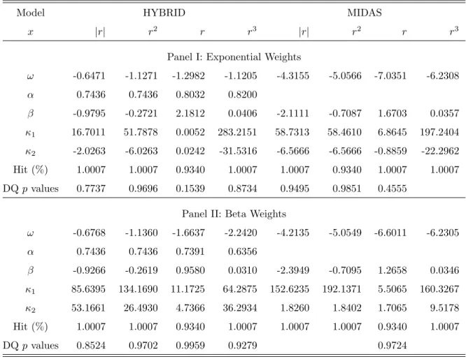
Table 2.2 shows the estimated parameters obtained from HYBRID quantile models and MIDAS quantile models for 1% VaRs. The models perform similarly by looking at

in-sample Hit and DQ tests for 1% VaRs.

(41)

2.4 Quantile Distribution Fits

Wu and Perloff (2005), Wu (2006) and Wu and Perloff (2007) fits densities to quan-tiles. This is an interesting aspect if we have several conditional quantiles and we want to use them to find the conditional density of either returns or standard returns by fitting quantiles to a density. We call this method Quantile Distribution Fits.

Assume we have conditional quantilesQr_t(p, θq) for a selection ofp-values and

deter-mined by a parameter vector θq for return r at time t. The Qr_t(p, θq) can be obtained

by quantile regression method like CAViaR, MIDAS Quantile regression, and HYBRID

Quantile regression. Then the conditional distribution of r at time t can be found by

solving

min

θd

1

N

X

p=1

[Qr_t(p, θq)−qt(p, θd)]2, ∀t ∈ {1, ..., T} (2.18)

whereθd_{is the parameters to be estimated,}_N _{is the number of quantiles used in finding}

conditional distribution, andqt(p, θd) is the quantile function of selected distribution.

For the choice of qt(p, θd), we can pick a rich family of distributions, like the

Gener-alized Hyperbolic (GH) class which is characterized by five parameters. When further narrowed down to subclasses of four-, three-, or two-parameter distributions, yields widely used distributions such as the normal inverse Gaussian distribution, the hyper-bolic distribution, the variance gamma distribution, the generalized skewed t distribu-tion, the student t distribudistribu-tion, the gamma distribudistribu-tion, the Cauchy distribudistribu-tion, the normal distribution, etc. We can also use extreme value distributions like Generalized Extreme Value (GEV) distribution and Generalized Pareto (GP) distribution.

For the choice of N, we can in principle fit as many quantiles as we want. More

(42)

of too many moment conditions, which creates singularities.

By having the conditional distribution, we can further obtain Expected Shortfall (ES), an alternative measure of risk proposed by Artzner, Delbaen, Eber, and Heath

(1997). The Expected Shortfall is the expected value ofrwhen the threshold (i.e. VaR)

has been exceeded. It can be calculated by integral over the quantile functionqt(p, θd)

in our case. The αth Expected Shortfall is defined as follows

ES_tα =Et(rt|rt< qt(α, θd)) =

1

α Z α

0

qt(γ, θd)dγ (2.19)

where 0< α <1.

We would like to compare the Expected Shortfall obtained using the fitted pa-rameters of quantile distribution fits with the regression based Expected Shortfall for CaViaR or other quantile models(Manganelli and Engle (2001)). The regression based Expected Shortfall is defined as follows

rt =δQrt(p, θ q_{) +}_η

t, rt< Qrt(α, θ

q₎ _(2.20)

ˆ

ESα_t = ˆE_tα(rt|rt< Qrt(α, θ

q_{)) = ˆ}_δQr

t(α, θ

q₎ _(2.21)

(43)

The results for comparison of Expected Shortfall using conditional distribution from quantile distribution fits and regression based Expected Shortfall are shown in Figure 2.3. The larger discrepancy for 1% ES may be caused by the smaller sample size in the regression.

We also test other distributions, including generalized pareto(GP) distribution. In general, quantile distribution fits with GEV performs better than with GP. Also, quan-tile distribution fits with t, skew t, and generalized hyperbolic distribution fails some-times due to a lack of analytic quantile functions. We also use other quantiles like 25%, 50%, and 75% quantiles, and the results are worse than using 10%, 20%, 30%, and 40% quantiles.

2.5 Simulation

In Section 2.5.1, we present results to compare the simulation results to compare conditional heteroskedasticity and quantiles.

Simulation of Conditional Heteroskedasticity versus Quantils

This section covers an extensive Monte Carlo simulation to compare conditional heteroskedasticity and quantiles. We first describe the conditional heteroskedasticity and quantiles models we use in this section.

We consider the conditional volatility as GARCH(1,1)

rt =σtεt (2.22)

σ_t2 =ω0+α0rt2−1+β0σt2−1 (2.23)

where E[εt|Ft−1] = 0, and E[ε2t|Ft−1] = 1. By specifying the density of εt, we define

(44)

If εt ∼ N(0,1), the model is Gaussian GARCH(1,1) and we denoted it as NOR.

The parameters to be estimated for this model is θ = (ω0, α0, β0).

If εt is Student’s t-distribution which has the probability density function given by

f(t|ν) = Γ

ν+1 2

√

νπΓ ν₂

1 + t

2

ν −ν+1₂

(2.24)

where ν > 2 is the number of degree of freedom and Γ is the Gamma Function. We

denote this Student’s t GARCH model as STDT. The parameters to be estimated for

this model is θ= (ω0, α0, β0, ν).

If εt is Skew t-distribution proposed by Hansen (1994) which has the probability

density function given by

g(z|ν, λ) = bc 1 + 1

ν−2

bz+a

1−λ

2!(−(ν+1)/2)

, z < −a/b (2.25)

=bc 1 + 1

ν−2

bz+a

1 +λ

2!(−(ν+1)/2)

, z ≥ −a/b (2.26)

whereν > 2,−1< λ <1, and

a = 4λcν−2 ν−1

b2 = 1 + 3λ2−a2

c= Γ

ν+1 2 p

π(ν−1)Γ (ν/2).

To ensure the mean and variance ofεt to be zero, a, b, and c must satisfy

E[Z] =a = 0

(45)

We denote this SKWE T GARCH model as SKEWT. The parameters to be estimated

for this model is θ = (ω0, α0, β0, ν, λ). Note there are only one free parameter λ to

be estimated, and it is the skewness parameter of this density.If λ >0, the density is

positively skewed and vice versa.

If εt is Generalized Hyperbolic Skew Student’st-distribution proposed by Aas and

Haff (2006) which has the probability density function given by

f(x|β, ν, µ, δ) =

21−2νδν|β| ν+1

2 _K_ν₊₁ 2

_q

β2 _δ2_{+ (}_x₋_µ₎2

exp (β(x−µ))

Γ ν₂√π

q

δ2_{+ (}_x₋_µ₎2

ν+1₂ , β 6= 0

(2.27)

= Γ

ν+1 2

√

πδΓ ν₂ "

1 + (x−µ)

2

δ2

#−(ν+1)/2

, β = 0 (2.28)

where ν > 4 to ensure finite variance. To ensure the mean and variance of εt to be

zero, the parameters must satisfy

E[X] =µ+ βδ 2

ν−2 = 0

V ar[X] = 2β 2_δ4

(ν−2)2(ν−4)+

δ2 ν−2 = 1

We denote this Generalized Hyperbolic Skew t GARCH model as GHST. The

param-eters to be estimated for this model isθ = (ω0, α0, β0, β, ν, µ, δ).

The skewness of the above density is

skew[X] = 2 (ν−4) 1/2

βδ

[2β2_δ2_{+ (}_ν₋_{2) (}_ν₋_4)]3/2

3 (ν−2) + 8β

2_δ2

ν−6

. (2.29)

It is time-invariant. To generate time-varying skewness in the simulation, we also

(46)

a AR(1) process.

νt =c+φνt−1+t (2.30)

βt==c+φβt−1+t (2.31)

wheret is white noise with variance k. We denote the Generalized Hyperbolic Skew t

GARCH with time-varying β model as GHYP1 and the Generalized Hyperbolic Skew

t GARCH with time-varying ν model as GHYP2. The parameters for this model is

θ = (ω0, α0, β0, β, ν, µ, δ, c, φ, k). The last three parameters are determined without estimation for both GHYP1 and GHYP2.

The last GARCH type model we consider is the model thatεt follows mixed normal

distribution with two components. We denote this model as MIXNOR. The parameters

to be estimated for this model is θ = (ω0, α0, λ1, λ2, µ1, µ2, σ1, σ2). These parameters

must satisfy conditions such that λ1+λ2 = 1, E(εt|Ft−1) = 0, and E(ε2t|Ft−1) = 1.

The single horizon quantile models we consider here are four CAViaR models

pro-posed by Engle and Manganelli (2004). Letrt be the return, andqt be theθth quantile

of rt. The symmetric Absolute Value CAViaR model, denoted as SAV, is

qt(β) = β1+β2qt−1(β) +β3|rt−1|. (2.32)

The Symmetric Square Value CAViaR model, denoted as SSV, is

(47)

The Asymmetric Slope CAViaR model, denoted as AS, is

qt(β) =β1+β2qt−1(β) +β3(rt−1)++β4(rt−1)

−

. (2.34)

The Adaptive CAViaR model, denoted as AD, is

qt(β1) =qt−1(β1) +β1

1 + exp G[yt−1−qt−1(β1)]−1−θ , G= 10. (2.35)

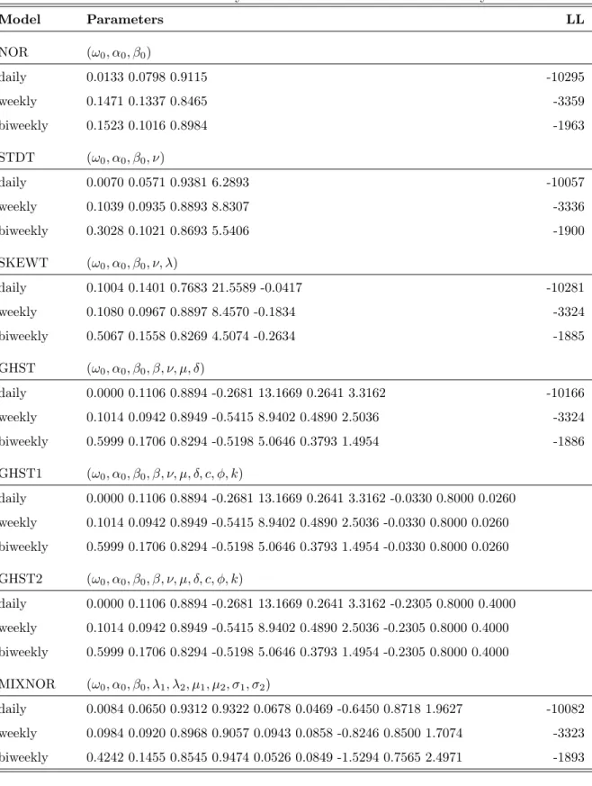
Table 2.4 provides a summary of notations and descriptions of these models used in the simulation and estimation.

We simulate data using seven different data generating processes (i.e. NOR, STDT, SKEWT, GHYP, GHYP1, GHYP2, and MIXNOR). For the data generating processes NOR, STDT, SKEWT, GHYP and MIXNOR, the parameters used in the simulations are obtained by estimating 1982-2011 S&P 500 returns using the models accordingly.

For GHYP1 and GHYP2, we use time-varying β and ν generated by AR(1) processes,

respectively, while other parameters remain the same as GHYP. For each data gener-ating process, we simulate 1000 samples with length 2500.

Table 2.4 shows all the parameter choices used in the simulation. They are obtained by estimating 1982-2011 S&P 500 daily, weekly, and biweekly returns using the models accordingly. The last column is log likelihood obtained through the estimations. For daily data, STDT model is the best model by looking at this criteria. For weekly and biweekly data, MIXNOR and GHYST provide the best estimation results, respectively. For each sample, we estimate conditional heteroskedasticity models(NOR, STDT, SKEWT, GHYP, and MIXNOR) and CaViAR models(5%, 25%, and 75% quantiles).

The performances of model estimations are evaluated through the estimates of ˆσt and

(48)

questions what are the true and estimated conditional Value at risk from GARCH type models, and how to find out the conditional volatility from the quantile models.

For CAViaR models, the ˆσ2

t is estimated throughc×IQRˆ

2

, where cis a parameter

estimated through the interquartile range of each DGP3 _and _IQR_ˆ _{is the estimates of}

interquartile range. For conditional heteroskedasticity models, the 5% VaR is estimated

through qtrue

5% σttrue, where qtrue5% is the 5% quantile of each DGP.

The measures we use to compare ˆσtareQLIKE andM SEpropproposed by Patton

(2011). The definitions are as follows.

QLIKE = 1

T

X

t=1

log ht

ˆ

σ2

t

+σˆ

2

t

ht

−1

, (2.36)

M SEprop= 1

T

X

t=1

ˆ

σ_t2 ht

−1 2

, (2.37)

and ht = (σttrue)2. where QLIKE is normalized to yield zero when the estimated

volatility is equal to the true volatility. A smaller value of QLIKE means better

estimation. We compare the estimates of 5% VaR using Mean squared error. The results of comparisons are shown in Table 2.5 - Table 2.7.

Table 2.5 shows the comparison of σt usingQLIKE. For the simulation with data

generating process NOR, the CaViaR quantile models SAV and AS perform compa-rably to the true model NOR. For data generating process STKEWT, the CaViaR quantile model SAV performs comparably to the true model SKEWT. GARCH type model NOR and CaViaR model AS perform similarly and slightly worse than the true model SKEWT. For data generating process GHST, the true model performs the best, then followed by other GARCH type models. In this case, the CaViaR quantile models

(49)

do not show advantage over the GARCH type models. But for data generating pro-cess GHYP2, the CaViaR quantile models SAV performs comparably with estimated through GHYP and performs better than other GARCH type models. For data gen-erating process MIXNOR, CaViaR quantile model SAV performs better than NOR, STDT, and GHST, and worse than SKEWT and the true model MIXNOR. Overall, CaViaR model SAV performs consistently very well for a variety of data generating process.

Table 2.6 shows the comparison of σtusing M SEprop. For data generating process

NOR, SAV performs similarly to NOR by looking M SEprop. For data generating

process STDT, CaViaR quantile models SAV, SSV and AS perform even better than the true model STDT. For data generating process SKEWT, the CaViaR model SAV and AS perform better than the true model SKEWT. For data generating process GHST, the true model performs the best, then followed by other GARCH type models. In this case, the CaViaR quantile models do not show advantage over the GARCH type models

as using the measure of QLIKE. For data generating process MIXNOR, CaViaR

quantile model SAV performs the best. Overall, using M SEprop as criteria, CaViaR

quatile models shows even more advantages than GARCH type models compared with

using QLIKE.

In conclusion, for estimation of ˆσt, CAViaR Models (SAV, SSV, AS) are better than

GARCH type models when there are fat tail, skewness or time-varying skewness in the data.

Table 2.7 shows the comparison of VaR using MSE. And the findings can be sum-marized as follows. For estimation of VaR, some of the GARCH type models are better

than CaViaR Models. This makes sense since the estimation of q5% is less accurate

(50)

2.6 Conclusion

We introduce a generic of HYBRID quantile regression models and use the measure

of in-sampleHitandDQtests(Manganelli and Engle (2001)) to check the performance

of our models compared with MIDAS quantile regression models. For the estimation of 5% VaRs, the HYBRID quantile regression models are prefered. For 1% VaRs, there two types of models provide similar results.

We propose a method to find conditional distributions based on quantile regres-sions called Quantile Distribution Fits. This method allows us to calculate Expected Shortfall, and other properties, which is very useful for risk management. We compare the results of quantiles/Value at Risk by quantile regressions and quantile distribu-tion fits. We also study the expected shortfall using condidistribu-tional distribudistribu-tion obtained by quantile distribution fits with the regression based expected shortfall for quantiles regressions. The results suggest that Quantile Distribution Fits is a very promising alternative method for risk management.

For estimation of ˆσt, CAViaR Models (SAV, SSV, AS) are better than GARCH

type models when there are fat tail, skewness or time-varying skewness in the data. For estimation of VaR, some of the GARCH type models are superior than CaViaR

Models. This may arise from the fact that the estimation of q5% is less accurate than

say the estimations ofq25% and q75% for skewness measures.

2.7 Tables and Figures

(51)

Table 2.1: Hybrid quantiles and MIDAS quantiles for 5% VaR

Model HYBRID MIDAS

x |r| r2 _r _r3 _|_r_| _r2 _r _r3

Panel I: Exponential Weights

ω -0.2255 -0.5661 -0.6124 -0.9906 -1.8101 -2.8321 -3.8394 -3.4571

α 0.7201 0.7692 0.8408 0.6911

β -1.0231 -0.1710 1.0062 0.0407 -2.0661 -0.4581 0.8005 0.0466

κ1 82.4187 18.8972 1.3519 223.6761 58.4813 4.2246 335.1269 239.4319

κ2 -11.5922 -2.4032 -0.1867 -31.5316 -6.5666 -0.4442 -47.6295 -29.9681

Hit (%) 4.9366 5.0033 5.0033 5.0033 5.0033 5.0033 5.0033 4.9366

DQpvalues 0.9370 0.8868 0.5496 0.8883 0.0172 0.9630 0.0000 0.0428

Panel II: Beta Weights

ω -0.2018 -0.5769 -0.8949 -0.7841 -1.9384 -2.8254 -3.8074 -3.4578

α 0.7153 0.7692 0.7559 0.7565

β -1.0891 -0.1648 0.8543 0.0290 -1.8649 -0.4500 0.7887 0.0466

κ1 70.3929 62.6558 10.5647 53.9638 152.6235 221.1039 21.8558 128.1018

κ2 44.9371 37.6604 4.4327 29.8219 1.8488 1.8442 10.8169 3.2954

Hit (%) 5.0033 4.9366 4.9366 5.0033 5.0700 5.0033 5.0033 5.0033

(52)

Table 2.2: Hybrid quantiles and MIDAS quantiles for 1% VaR

Model HYBRID MIDAS

x |r| r2 _r _r3 _|_r_| _r2 _r _r3

Panel I: Exponential Weights

ω -0.6471 -1.1271 -1.2982 -1.1205 -4.3155 -5.0566 -7.0351 -6.2308

α 0.7436 0.7436 0.8032 0.8200

β -0.9795 -0.2721 2.1812 0.0406 -2.1111 -0.7087 1.6703 0.0357

κ1 16.7011 51.7878 0.0052 283.2151 58.7313 58.4610 6.8645 197.2404

κ2 -2.0263 -6.0263 0.0242 -31.5316 -6.5666 -6.5666 -0.8859 -22.2962

Hit (%) 1.0007 1.0007 0.9340 1.0007 1.0007 0.9340 1.0007 1.0007

DQpvalues 0.7737 0.9696 0.1539 0.8734 0.9495 0.9851 0.4555

Panel II: Beta Weights

ω -0.6768 -1.1360 -1.6637 -2.2420 -4.2135 -5.0549 -6.6011 -6.2305

α 0.7436 0.7436 0.7391 0.6356

β -0.9266 -0.2619 0.9580 0.0310 -2.3949 -0.7095 1.2658 0.0346

κ1 85.6395 134.1690 11.1725 64.2875 152.6235 192.1371 5.5065 160.3267

κ2 53.1661 26.4930 4.7366 36.2934 1.8260 1.8402 1.7065 9.5178

Hit (%) 1.0007 1.0007 0.9340 1.0007 1.0007 1.0007 0.9340 1.0007

5357.pdf

STATISTICAL ANALYSIS OF FINANCIAL TIME SERIES AND

RISK MANAGEMENT

Abstract

Acknowledgments

Table of Contents

. . . .

List of Figures

List of Tables

Chapter 1

Asymptotic Properties of Quantile-based Conditional

Skewness Models for Asset Pricing

1.1 Introduction

1.2 The Asset Pricing Model

1.3 The Empirical Quantile Model

1.4 Asymptotic Properties

1.5 Conclusion

1.6 Proofs

Chapter 2

Dynamic Quantile Models for Risk Management

2.1 Introduction

2.2 The Generic Setup

2.3 Dynamic Quantile Models

2.4 Quantile Distribution Fits

2.5 Simulation

2.6 Conclusion

2.7 Tables and Figures