NATIONAL OPEN UNIVERSITY OF NIGERIA
COURSE CODE: CIT 844
COURSE TITLE:
COURSE
GIUDE
ADVANCED DATABASE MANAGEMENT SYSTEM
Course Developer/Writer Dr. Olusegun Folorunso
Department of Computer Science University of Agriculture
Abeokuta
Programme Leader Prof. Afolabi Adebanjo
National Open University of Nigeria
NATIONAL OPEN UNIVERSITY OF NIGERIA
CIT 844 ADVANCED DATABASE MANAGEMENT SYSTEM National Open University of Nigeria
Headquarters
14/16 Ahmadu Bello Way Victoria Island
Lagos
Abuja Office
No. 5 Dar es Salaam Street Off Aminu Kano Crescent Wuse II, Abuja
Nigeria
e-mail: [email protected] URL: www.nou.edu.ng
Published by
National Open University of Nigeria Printed 2009
ISBN: XXX-XXX-XXX-X All Rights Reserved
CONTENTS PAGE
Introduction……….…….. v
What you will Learn in this Course ……….……… v
Course Aims……….……… vi
Course Objectives……….……… vi
Working through this Course ………..………. vi
Course Materials……….……….. vi
Online Materials……….……….. vii
Study Units……….……….. vii
Equipments……….………. viii
Assessment……….. ix
Tutor-Marked Assignment………... ix
Course Overview ………..….. x
How to Get the Most from this Course ………..………. x
Introduction
The course, Advanced Database Management System, is a core course for students studying towards acquiring the Master of Science in Information Technology. In this course we will study about the Database Management System as a key role in Information Management. Various principles of database management system (DBMS) as well as its advanced features are discussed in this course. This course also considers distributed databases and emerging trends in database system.
The overall aim of this course is to introduce you to various ways of designing and implementing database systems, features and distributed databases. In structuring this course, we commence with the basic design and implementation of relational databases.
There are four modules in this course, each module consists of units of topics that you are expected to complete in 2 hours. The four modules and their units are listed below.
What You Will Learn in this Course
The overall aims and objectives of this course provide guidance on what you should be achieving in the course of your studies. Each unit also has its own unit objectives which state specifically what you should be achieving in the corresponding unit. To evaluate your progress continuously, you are expected to refer to the overall course aims and objectives as well as the corresponding unit objectives upon the completion of each.
Course Aims
The overall aims and objectives of this course will help you to:
1. Develop your knowledge and understanding of the underlying principles of Relational Database Management System
2. Build up your capacity to learn DBMS advanced features
3. Develop your competence in enhancing database models using distributed databases 4. Build up your capacity to implement and maintain an efficient database system using emerging trends.
Course Objectives
Upon completion of the course, you should be able to:
1. Describe the basic concepts of Relational Database Design 2. Explain Database implementation and tools
3. Describe SQL and Database System catalog.
4. Describe the process of DB Query processing and evaluation. 5. Discuss the concepts of transaction management.
6. Explain the Database Security and Authorization. 7. Describe the design of Distributed Databases. 8. Know how to design with DB and XML.
9. Describe the basic concept of Data warehousing and Data mining
10. Discuss the emerging Database Models Technologies and Applications
Working through this Course
We designed this course in a systematic way, so you need to work through it from Module one, Unit 1 through to Module four, Unit 3.
This will enable you appreciate the course better.
Course Materials
Basically, we made use of textbooks and online materials. You are expected to I, search for more literature and web references for further understanding. Each unit has references and web references that were used to develop them.
Online Materials
Feel free to refer to the web sites provided for all the online reference materials required in this course.
The website is designed to integrate with the print-based course materials. The structure follows the structure of the units and all the reading and activity numbers are the same in both media.
Study Units
Course Guide
Module 1: Database Design and Implemental
Unit 1: Relational Database Design Unit 2: Database Implementation & Tools Unit 3: Advance SQL
Unit 4: Database System Catalog
Module 2: DBMS Advance Features
Unit 1: Query Processing & Evaluation
Unit 2: Transaction Management and Recovery Unit 3: Database Security & Authorization
Module 3: Distributed Databases
Unit 1: Enhanced Database Models Unit 2: Object Oriented Database Unit 3: Database and XML
Unit 4: Introduction To Data Warehousing Unit 5: Introduction to Data Mining
Module 4: Emerging Trends and Example of DBMS Architecture
Unit 2: Technologies and Applications Unit 3 PostgreSQL & Oracle
Module one describes Database Design and Implementation. Module Two explains the DBMS advanced features.
Module Three discusses the Distributed Database.
Module Four discusses Emerging trends in DBMS including technologies and applications.
Equipment
In order to get the most from this course, it is essential that you make use of a computer system which has internet access.
Recommended System Specifications:
Processor
2.0 GHZ Intel compatible processor 1GB RAM
80 GB hard drive with 5 GB free disk CD-RW drive.
3.5" Floppy Disk Drive TCP/IP (installed)
Operating System
Windows XP Professional (Service Pack 2) Microsoft office 2007
Norton Antivirus
Monitor* 19-inch
1024 X 768 Resolution 16-bit high color
*Non Standard resolutions (for example, some laptops) are not supported.
DBMS Tools
ORACLE PostgreSQL
Hardware
Open Serial Port (for scanner) 120W Speakers
Windows keyboard Laser printer
Hardware is constantly changing and improving, causing older technology to become obsolete. An investment in newer, more efficient technology will more than pay for itself in improved performance results.
If your system does not meet the recommended specifications, you may experience considerably slower processing when working in the application. Systems that exceed the recommended specifications will provide better handling of database files and faster processing time, thereby significantly increasing your productivity.
Assessment
The course, Advanced Database Management Systems entails attending a two-hour final examination which contributes 50% to your final grading. The final examination covers materials from all parts of the course with a style similar to the Tutor- marked
assignments.
The examination aims at testing your ability to apply the knowledge you have learned throughout the course, rather than your ability to memorize the materials. In preparing for the examination, it is essential that you receive the activities and Tutor-marked
assignments you have completed in each unit. The other 50% will account for all the TMA’s at the end of each unit.
Tutor-Marked Assignment
About 20 hours of tutorials will be provided in support of this course.
You will be notified of the dates, time and location for these tutorials, together with the name and phone number of your tutor as soon as you are allotted a tutorial group. Your tutor will mark and comment on your assignments, keep a close watch on your progress and on any difficulties you might encounter and provide assistance to you during the course. You must mail your TMAs to your tutor well before the due date (at least two working days are required). They will be marked by your tutor and returned to you as soon as possible.
The following might be circumstances in which you would find help necessary. You can also contact your tutor if:
you do not understand any part of the study units or the assigned readings you have difficulty with the TMAs
you have a question or problem with your tutor’s comments on an assignment or with the grading of an assignment
You should try your best to attend tutorials, since it is the only opportunity to have an interaction with your tutor and to ask questions which are answered instantly. You can raise any problem encountered in the course of your study. To gain maximum benefit from the course tutorials, you are advised to prepare a list of questions before attending the tutorial. You will learn a lot from participating in discussions actively.
Course Overview
This section proposes the number of weeks that you are expected to spend on the three modules comprising of 30 units and the assignments that follow each of the unit. We recommend that each unit with its associated TMA is completed in one week, bringing your study period to a maximum of 30 weeks.
How to Get the Most from this Course
In order for you to learn various concepts in this course, it is essential to practice. Independent activities and case activities which are based on a particular scenario are presented in the units. The activities include open questions to promote discussion on the relevant topics, questions with standard answers and program demonstrations on the concepts. You may try to delve into each unit adopting the following steps:
1. Read the study unit
2. Read the textbook, printed or online references 3. Perform the activities
4. Participate in group discussions
5. Complete the tutor-marked assignments 6. Participate in online discussions
Specific web address will be given for your reference. There are also optional readings in the units. You may wish to read these to extend your knowledge beyond the required materials. They will not be assessed.
Summary
The course, Advanced Database Management Systems is intended to develop your understanding of the basic concepts of database systems, thus enabling you acquire skills in designing and implementing Database Management Systems. This course also provides you with practical knowledge and hands-on experience in implementing and maintaining a system. We hope that you will find the course enlightening and that you will find it both interesting and useful. In the longer term, we hope you will get acquainted with the
ADVANCED DATABASE MANAGEMENT SYSTEM
MAIN COURSE
Course Developer/Writer Dr. Olusegun Folorunso
Department of Computer Science University of Agriculture
Abeokuta
Programme Leader Prof. Afolabi Adebanjo
National Open University of Nigeria
Course Coordinator National Open University of Nigeria
CIT 844 ADVANCED DATABASE MANAGEMENT SYSTEM
National Open University of Nigeria Headquarters
14/16 Ahmadu Bello Way Victoria Island
Lagos
Abuja Office
No. 5 Dar es Salaam Street Off Aminu Kano Crescent Wuse II, Abuja
Nigeria
e-mail: [email protected] URL: www.nou.edu.ng
Published by
National Open University of Nigeria Printed 2009
ISBN: XXX-XXX-XXX-X All Rights Reserved
CONTENTS PAGE
MODULE 1: Database Design and Implementation
Unit 1: Relational Database Design.
1.0 Introduction……… 1
1.1 Objectives………. 1
1.2 What is Relational Database?... 1
1.2.1 Relational Database Model Concept………. 1
1.2.2 Relational Constraints and Relational Database Schemas………... 6
1.2.3 Update operations and Dealing with Constraint Violations……….. 8
1.3 Relational Database Design……….. 18
1.3.1 The Entity Relational (ER) model………. 18
1.3.2 An Illustration of a Company Database Application……… 20
1.3.3 Entity Types, Entity Set, Attributes and keys………. 20
1.3.4 Entity Types, Entity Set, Key and Value Set………. 22
1.3.5 Pitfalls in a Relational Database Design……… 23
1.4 Normalization………. 29
1.5 Conclusion……….. 58
1.6 Summary……… 58
1.7 Tutor Marked Assignment………. 59
Unit 2: Database Implementation
2.0. Introduction……….. 61
2.1. Objectives………. 61
2.2. Conceptual Design……… 61
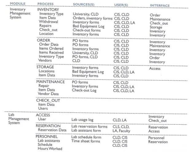
2.2.1 Information Sources and Users……….. 62
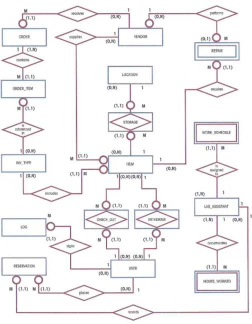
2.3. E-R Model Verification………. 63
2.4. Logical Design……… 70
2.5. Physical Design……….. 72
2.6. Implementation………... 74
2.6.1 Database Creation……… 74
2.6.2 Database Loading and Conversion………. 74
2.6.3 System Procedures……….. 75
2.7 Testing and Evaluation……… 75
2.7.1. Performance Measures………. 75
2.8 Security Measures………76
2.9. Operations……… 77
2.10 Conclusion………. 77
2.11 Summary……… 77
2.12 Tutor Marked Assignment………. 78
2.13 Further Readings……… 79
Unit 3: Advanced SQL.
3.0. Introduction……… 803.2. What is SQL?... 80
3.3. Using SQL on a Relational Database…….………... 81
3.4. SQL Statements……… 83
3.5. Conclusion……… 108
3.6. Summary……….. 108
3.7. Tutor Marked Assignment (TMA)……….. 108
3.8. Further Reading……… 109
Unit 4: Database System Catalogue
4.0. Introduction……….. 1104.1. Objectives………. 110
4.2. What is Database System Catalogue?... 110
4.3. Conclusion……… 111
4.4. Summary……….. 111
4.5. Tutor Marked Assignment (TMA)……… 111
4.6. Further Readings……….. 111
Module 2: Advanced Features and DBMS
Unit 1: Query Processing & Evaluation
1.0. Introduction...……….………. 1121.1. Objectives…..……….. 112
1.2. Query Interpretation……....……… 112
1.3. Equivalence of Expressions……… 113
2.2.1. Transaction Properties………. 129
2.2.2. Transaction Management with SQL……… 130
2.2.3. The Transaction Log………. 131
2.2.4 Types of Transaction Log Records………... 132
1.3.2. Natural Join Operations………. 115
1.3.3. Projection Operations……… 116
1.4. Estimation of Query-Processing Costs……… 117
1.5. Estimation Of Costs of Access Using Indices……….. 118
1.6. Join Strategies………. 120
1.6.1. Simple Iteration……… 121
1.6.2. Block-Oriented Iteration……….. 121
1.6.3. Merge-Join……… 123
1.6.4. Use of an Index………. 124
1.6.5. Three-Way Join………. 124
1.7. Structure of Query Optimizer………... 125
1.8. Conclusion………. 126
1.9. Summary……… 126
1.10. Tutor-Marked Assignment (TMA)……… 127
1.11. Further Readings……….. 127
Unit 2: Transaction Management & Recovery
2.0. Introduction……… 1282.1. Objectives……… 128
2.3. Concurrency Control……… 132
2.3.1. Concurrency control with Locking Methods……… 133
2.3.2. Types of Locks………. 133
2.3.3. Two-Phase Locking to Ensure Serializablility……….. 134
2.3.4. Deadlocks……….. 134
2.4. Concurrency Control with Time Stamping Methods……….... 134
2.5 Concurrency Control with Optimistic Methods……… 135
2.5.1 Optimistic Concurrency Control phases……… 135
2.6. Database Recovery Management………. 135
2.7. Conclusion……….. 136
2.8. Summary……….. 136
2.9. Tutor-Marked Assignment (TMA)……….. 136
2.10. Further Readings……….. 137
Unit 3: Database Security &Authorization
3.0. Introduction……….1383.1. Objectives………... 138
3.2. Security and Integrity Violations……… 138
3.3. Authorization & Views……….. 139
3.4. Integrity Constraints……… 143
3.5. Encryption………145
3.6. Statistical Databases……… 147
3.7. Conclusion………... 148
3.10. Further Readings………. 149
Module 3: Distributed Databases
Unit 1: Enhanced Database Model
1.0. Introduction………. 1501.1. Objectives……… 150
1.2. Distributed Databases………. 150
1.3. Structure of Distributed Databases………. 151
1.4. Trade-offs in Distributing the database………... 153
1.4.1 Advantages of Data Distribution……….. 153
1.4.2. Disadvantages of Data Distribution……….. 154
1.5. Design of Distributed Databases………. 154
1.5.1 Data Replication……….. 155
1.5.2 Data Fragmentation………. 155
1.5.3 Data Replication and Fragmentation……….. 159
1.6. Transparently and Autonomy……… 159
1.6.1 Naming and local Autonomy………. 160
1.6.2 Replication and Fragmentation Transparency……….. 160
1.6.3 Location Transparency………. 161
1.6.4 Complete Naming Scheme……….. 161
1.6.5 Transparency and Update to Replicated Data……….. 161
1.7. Distributed Query Processing………. 163
1.7.2 Simple Join Processing……… 163
1.7.3 Join Strategies……….. 164
1.7.4 Semijoin Strategies……… 164
1.8. Recovery in Distributed Systems………. 166
1.8.1 System Structure……….. 166
1.8.2 Robustness………. 167
1.8.3 Commit Protocols……… 168
1.9. Concurrency Control……….. 170
1.9.1 Locking Protocols……… 170
1.9.2 Time Stamping……… 173
1.10. Deadlock Handling……… 174
1.10.1 Centralized Approach………... 175
1.10.2 Fully Distributed Approach………. 177
1.11. Coordinator Selection……… 179
1.11.1 Backup Coordinators……… 180
1.11.2 Election Algorithms………. 180
1.12. Conclusion………. 181
1.13. Summary……… 181
1.14. TMA……….. 182
1.15. Further readings………. 183
Unit 2: Object Orientated Database
2.0. Introduction………. 1842.3. Object-Oriented Database Design………. 185
2.4. How OO Concept has Influenced the Relational Model……….. 187
2.5 Conclusion……….. 190
2.6 Summary……….. 190
2.7 TMA……….. 190
2.8 Further Readings……… 190
Unit 3: Database and XML
3.0 Introduction……….. 1913.1 Objectives……… 191
3.2 Define the Purpose of XML……… 191
3.3 XML Trees……… 194
3.4 XML Syntax Rules……… 196
3.5 XML Elements……….. 198
3.5.1 XML Naming Rules……… 199
3.6 XML Attributes……… 200
3.7. Conclusion……… 206
3.8 Summary………. 206
3.9. TMA………..… 206
3.10 Further Reading………... 206
Unit 4: Introduction to Data Warehousing
4.0 Introduction ……….. 2084.1 Objective……….. 208 4.2. What is Data Warehousing?... 208
4.3. Data Warehouse Architectures……….. 209
4.3.1. Data Warehouse Architecture (Basic)………. 210 4.3.2. Data Warehouse Architecture (With a Staging Area)………. 210 4.3.3.2. Data Warehouse Architecture (With a Staging Area and Data Mart) 211 4.4. Logical Versus Physical Design in Data Warehouse………. 212
4.5. Data Warehousing Schema……… 213
4.6 Data Warehousing Objects……… 214
4.6.1 Fact Tables……….. 214
4.6.2 Dimension Tables……… 214
4.7. Summary……… 220 4.8. Conclusion………. 220 4.9. TMA………... 220
4.9. Further Readings……… 220
Unit 5: Introduction to Data Mining
5.0. Introduction ……… 221
5.1. Objectives……… 221
5.2. Data Mining Uses……… 221
5.3. Data Mining Functions……… 223
5.4 Data Mining Technologies………. 224
5.6. Conclusion………. 226 5.7. TMA……….. 226
5.8. Further Readings………. 226
Module 4: Emerging Trends and Examples of DBMS Architecture
Unit 1: Emerging Database Models1.0. Introduction………. 227
1.1 Objectives……… 227 1.2. Limitations of Conventional Databases………. 227 1.3. What is Multimedia Database?... 228 1.4. Temporal Databases: Modelling Temporal data: Temporal SQL…………. 230
1.4.1 Introduction……… 230
1.4.2 Temporal Data Semantics……… 230
1.4.3 Temporal Data Models and Query Languages……….. 232
1.5 Temporal DBMS Implementation……… 236
1.5.1 Query Processing……… 236
1.5.2 Implementing Algebraic Operators……… 237 1.5.3 Indexing Temporal Data……… 238 1.6 Outlook………. 238 1.7 Conclusion……… 241 1.8 Summary……….. 241
1.9. Tutor Marked Assignment……….. 241
Unit 2: The Major Application Domains
2.0 Introduction………. 243 2.1 Objectives……… 243 2.2 Database on the World Wide Web……….. 243
2.3 GIS Application……… 243
2.3.1 Specific GIS Data Operations……… 244 2.3.2 An Example of A GIS: Arc-Info……… 245
2.4 GENOME Data Management……… 246
2.4.1 Biological Sciences and Genetics……….. 246 2.4.2 Characteristics of Biological Data………. 247 2.4.3 The Human GENOME Project and Existing Biological Databases.. 249
2.5 Digital Libraries………. 250
2.6 Conclusion………. 251 2.7 Summary……….. 251
2.8 Further Reading………. 252
Unit 3 PostgreSQL
3.0 Introdection……… 253 3.1 Objectives……….. 253
3.2 What is PostgreSQL……….. 253
3.3 PostgreSQL and other DBMS’s………. 254
3.4 Open Source Software……… 259
3.7 Tutor Marked Assignment……….. 259
3.8 Further Reading……….. 259
MODULE
1:
DATABASE
DESIGN
&
IMPLEMENTATION
UNIT
1:
RELATIONAL
DATABASE
DESIGN
1.0 INTRODUCTION
This unit discusses extensively on relational data model. The model was first introduced
by Ted Codd of IBM research in 1970 in a classic paper, and attracted immediate
attention due to its simplicity and mathematical foundations. The model uses the
concept of mathematical relation, which looks somewhat like a table of values, as its
basic building blocks, and has its theoretical basics in set theory and first order predicate
logic. In this unit, we will discuss the basic characteristics for the relational model and its
normalization processes. The model has been implemented in a large number of
commercial systems over the last years.
1.1 OBJECTIVES.
To understand the relational database model.
To understand the concepts of normalization in database design
1.2 WHAT IS RELATIONAL DATABASE?
A relational database is a database that groups data using common attributes found in
the data set. The resulting "clumps" of organized data are much easier for people to
understand. For example, a data set containing all the real estate transactions in a town
can be grouped by the year the transaction occurred; or it can be grouped by the sale
price of the transaction; or it can be grouped by the buyer's last name; and so on. Such a
grouping uses the relational model (a technical term for this is schema). Hence such a
database is called a "relational database”. The software used to do this grouping is
called a relational database management system. The term "relational database" often
refers to this type of software. Relational databases are currently the predominant
choice in storing financial records, manufacturing and logistical information, personnel
data and much more.
The relational model represents the database as a collection of relations. Informally,
each relation resembles a table of values or, to some extent a “flat” file of record. For
example, the university database of files that was shown earlier is considered to be in
the relational model. However, there are important differences between relations and
files, as we shall soon see.
When a relation is thought of as a table of values, each row in the table represents a
collection of related data values. In the relational model, each row in the table
represents a fact that typically corresponds to a real‐world entity or relationship. The
table name and column names are used to help in interpreting the meaning of the row
which represents facts about a particular student entity. The column names ‐ Name,
Student, Number, Class, Major ‐ specify how to interpret the data values in each row,
based on the column each value is in. All values in a column are of the same data type.
In the formal relational model terminology, a row is called a tuple, a column header is
called an attribute, and the table is called a relation. The data type describing the types
of values that can appear in each column is called a domain. We now define these
terms – domain, tuple, attribute, and relation – more precisely.
Domains, Attributes, Tuples, & Relations
A domain D is a set of atomic values. By atomic we mean that each value in the domain
is indivisible as far as the relational model is concerned. A common method of specifying
a domain is to specify a data type from which the data values forming the domain are
drawn. It is also useful to specify a name for the domain, to help in interpreting its
values. Some examples of domains follow:‐
GSM phone‐numbers: The set of 11‐digit numbers valid in the Nigeria. E.g.
0803‐5040‐ 707.
Local‐phone‐numbers: The set of 6‐digit phone numbers valid within a particular
area code in Nigeria. E.g. 245290
Names: The set of names of persons.
Grade‐point‐averages: Possible values of computed grade point averages; each
must be a real (floating point) number between 0 and 5
Employee‐ages: Possible ages of employees of a company, each must be a value
between 18 and 65 years old
Academic‐department‐codes: The set of academic department codes, such as CSC,
ECON, and PHYS, in a university.
The preceding are called logical definitions of domains. A data type of format is also specified
on each domain. For example, the data type for the domain GSM phone‐numbers can be
declared as a character string of the form (dddd)dddd‐ddd, e.g. 0803‐5640‐707 where each d is
a data type. For Employee‐ages, the data type is an integer number between 18 and 65, for
Academic‐department‐names, the data type is the set of all character strings that represent
valid department names. A domain is thus given a name, data type, and format. Additional
information for interpreting the values of a domain can also be given. For example, a numeric
domain such as person‐weights should have the units of measurement ‐ kilograms.
A relations schema
, denoted by , is made up of a relation name R and a list of attributes .
Each attributes is the name of a role played by some domain
in the relation schema
.
is called the domain of
, and is denoted by . A relation schema is used to describe a relation
is called the name of this relations. The degree of a relation is the number of attributes
of its relation schema.
An example of a relation schema for a relation of degree 7, which describes university students,
is the following:
STUDENT (Name, SSN, HomePhone, Address, OfficePhone, Age, GPA)
Attributes
Relation Name
Student Name Ssn Home phone Address Office Phone Age Gpa
Tuples
Olumide Enoch 305‐61‐2435 080‐3616 2, Kings way Rd. null 19 4.21
Adamson Femi 381‐62‐1245 080‐4409 125, Allen Avenue null 18 3.53
Yisa Ojo 22‐11‐2320 null 34,Obantoko Road 749‐1253 25 2.89
Charles Olumo 489‐22‐1100 080‐5821 256 Grammar School 749‐6492 28 3.93
Johnson Paul 533‐69‐1238 0804461 7384, Paul Job Road null 19 3.25
For this relation schema, STUDENT is the name of the relation, which has seven attributes.
We can specify the following previously defined domains for some of the attributes of the STUDENT relations:
A relation or relation state of the relation schema also denoted by
, is a set of n‐tuples . Each n‐tuple t is an ordered list of n values
,
where each value , is an element of or is a special null value. The
value in tuple t, which correspondence to the attribute is referred to as .
The terms relation intension for the schema and relation extension for a relation state
are also commonly used.
Table 1.0 shows an example of a STUDENT relation, which corresponds to the STUDENT schema
specified above. Each tuple in the relation represents a particular student entity. We display the
relation as a table, where each tuple is shown as a row and each attribute corresponds to a
column header indicating a role or interpretation of the values in that column. Null values
represent attributes whose values are unknown or do not exist for some individual STUDENT
The above definitions of a relation can be restated as follows. A relation is a
mathematical relation of degree n on the domains ,
which is a subset of the Cartesian product of the domains that define :
The Cartesian product specifies all possible combinations of values from the underlying
domains. Hence, if we denote the number of values or cardinality of a domain D by |D|, and
assume that all domains are finite, the total number of tuples in the Cartesian product is:
Characteristics Of Relations
The earlier definition of relations implies certain characteristic that makes a relation different
from a file or a table. We now discuss some of these characters.
Ordering of Tuples in a Relation: A relation is defined as a set of tuples. Mathematically,
elements of a set have no order among them; hence tuples in a relation do not have any
particular order. However in a file, records are graphically stored on disk so there always
is an order among the records. This ordering indicates first, second, and last records in
the file. Similarly, when we display a relation as a table, the rows are displayed in a
Tuple ordering is no part of a relation definition, because a relation attempts to
represent facts at a logical or abstract level. Many logical orders can be specified on a
relation, for example, tuples in this STUDENT relation in Table 1.0 could be logically
ordered by values of Name, SSN, Age, or some other attribute. The definition of a
relation does not specify any order, there is no preference for one logical ordering over
another. Hence, the relation displayed in Table 1.1 is considered identical to the one
shown in Table 1.0. When a relation is implemented as a file, a physical ordering may be
specified on the records of the file.
Ordering of values within a tuple, and an alternative definition of a relation: According to
the preceding definition of a relation, an n‐tuple is an ordered list of n values, so the
ordering of values in a tuple and hence of attributes in a relation schema.
An alternative definition of relation can be given, making the ordering of value in a tuple
unnecessary. In this definition, a relation schema R = (A1,A2,..., An) is a set of attributes
and relation is a finite set of mappings r = [t1,t2,…,tm], where each tuple is a mapping
from R to D, and D is the union of attribute domains; that is, .
Table 1.1. The relation STUDENT from Table 1.0, with a different order of tuples.
Student Name Ssn Home
phone Address
Office
Phone Age Gpa
Tuples
Olumide Enoch 305‐61‐2435 080‐3616 2, Kings way Rd. Null 19 4.21
Adamson Femi 381‐62‐1245 080‐4409 125, Allen Avenue null 18 3.53
Yisa Ojo 22‐11‐2320 Null 34,Obantoko Road 749‐1253 25 2.89
Charles Olumo 489‐22‐1100 080‐5821 256, Grammar School 749‐6492 28 3.93
Johnson Paul 533‐69‐1238 0804461 7384, Paul Job Road null 19 3.25
In this definition, t(A1) must be in dom(A1) for for each mapping t in r. Each mapping is
called a tuple.
t=<(Name; Yisa Ojo), (SSN,422‐112320), (HomePhone, null), (Address, 34 Obantoko Road). (Office Phone, 749‐1253), (GPA, 2.89), (HomePhone, null) >
749‐1253), (GPA, 2.89), (HomePhone; null)> Page | xxxi
Figure 1.0 Two identical tuples when order of attributes and values in not
According to this definition, a tuple can be considered as a set of (<attribute>, <value>) pairs,
where each pair gives the value of the mapping form an attributes A1 to a value v1 from
dom(A1). The ordering of attributes is not important, because the attribute name appear with
its value. By this definition, the two tuples shown in figure 1.0 are identical. This makes sense at
an abstract or logical level, since they are really in no reason to prefer having one attribute
value appear before another in a tuple.
When a relation is sense at an abstracts are physically ordered as fields within a records. We
will use the first definition of relation, where the attributes and the values within tuples are
ordered, because it simplifies much of the notation. However, the alternative definition given
here is more general.
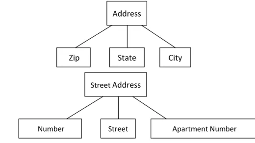
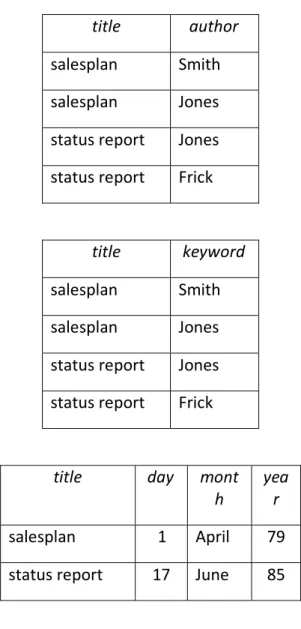
Values in the Tuples: Each value in a tuple is an atomic value; that is, it is not divisible into
components within the framework of the basic relational model. Hence, composite and
multi‐valued attributes are not allowed. Much of the theory behind the relational model
was developed with this assumption in mind, which is called the first normal form
assumption. Multi‐valued attributes must be represented by separate relations, and
composite attributes are represented only by their simple component attributes. Recent
research in the relational model attempt to remove these restrictions by using the
concepts of no first normal form or nested relations.
Interpretation of a Relation: The relation schema can be interpreted as a declaration or a
type of assertion. For example, the schema of the STUDENT relation of Table 1.0 asserts
that, in general, student entity has a Name, SSN, Home phone, Address, Office phone,
Age, and GPA. Each tuple in the relation can then be interpreted as a fact or a particular
instance of the assertion. For example, the first tuple in Table 1.0 asserts the fact that
there is a STUDENT whose name is Olutunde Enoch, SSN is 305‐61‐2435, Age in
19 and so on.
Notice that some relations may represent facts about entities, whereas other relations may
represent fact about relationship. For example, a relation schema MAJORS (Student SSN,
Department Code) asserts that students major in academic department, a tuple in this relation
relates a student to his or her major department. Hence, the relational model represents fact
about both entities and relationship uniformly as relations.
1.2.2 Relational Constraints And Relational Database Schemas
In this unit, we discuss the various restrictions on data that can be specified on
relational database schema in the form of constraints. These include domain constraints, key
strains, called data dependencies (which include functional dependencies and multi‐valued
dependencies), are used mainly for database design by normalization.
Domain constraints
Domain constraints specify that the value of each attribute A must be an atomic value from the
domain dom(A). We have already discussed the ways in which domains can be specified above.
The data types associated with domains typically include standard numeric data type for
integers (such as short‐integer, long‐inter) and real number (float and double‐precision float).
Character, fixed‐length strings, and variable‐length strings are also available, as are date, time,
timestamp, and money data types. A sub‐range of values from a data type or an enumerated
data type may describe other possible domains where all possible values are explicitly listed.
Key constraints and constraints on null
A relation is defined as a set of tuples. By definition, all elements of a set are distinct, hence, all
tuples in relation must also be distinct. This means that no two tuples can have the same
combination of values for all their attributes. Usually, there are other subsets of attributes of a
relation schema R with the property that no two tuples in any relation state r of R should have
the same combination of values for these attributes. Suppose that we denote one such subset
of attributes by SK; then for any two distinct tuples t1 and t2 in a relation sate r or R, we have
the constraint that t1[SK]1t2[SK].
Any such set attributes SK is called a superkey of the relation schema R. A superkey SK specifies
a uniqueness constraint that no two distinct tuples in a state r of R can have the same value for
SK. Every relation has at least one default superkey the set of all its attributes. A superkey can
have redundant attributes, however, so a more useful concept is that of a key, which has no
redundancy. A key K of a relation schema R is a superkey of R with the additional property that
removing any attribute A from K leaves a set of attributes K that is not a superkey of R. Hence, a
key is a minimal superkey‐ that is, a superkey from which we cannot remove any attributes and
still have the uniqueness constraint hold.
For example, consider the STUDENT relation of Table 1.0 the attribute set (SSN) is a key of
STUDENT because no two student tuples can have the same value for SSN. Any set of attributes
that include SSN for example, (SSN, Name, Age) is a superkey. However, the superkey (SS,
Name, Age) is not a key for STUDENT, because removing Name or Age of both from the set still
leaves us with a superkey.
The value of key attribute can be used to identify uniquely each tuples in the relation. For
Bayer in the STUDENT relation. Notice that a set of attributes constituting a key is a property of
the relation schema; it is a constraint that should hold on every relation state of the schema. A
key is determined from the meaning of the attributes, and the property is time‐invariant; it
must continue to hold when we insert new tuples in the relation. For example, we cannot and
should not designate the Name attribute of the student relation in Table 1.0 as a key, because
there is no guarantee that two student with identical names will never exist.
In general, a relation schema may have more than one key. In this case, each of the keys is
called a candidate key. For example, the CAR relation in Table 1.2 has candidate keys: License
Number and Engine Serial Number. It is common to designate the candidate key as the primary
key of the relation. This is the key whose value is used to identify tuples in the relation. We use
the convention that the attributes that form the primary key of a relation schema are
underlined, as shown in Table 1.2. Notice that, when a relation schema has several candidate
key, the choice of one to become primary key is arbitrary; however, it is usually better to
choose a primary key with a single attribute or a small number of attributes. Another constraint
on attributes specifies whether null values are or are not permitted. For example, if every
student tuple must have a valid non‐null value for the Name attribute, then Name of student is
constrained to be NOT null.
Table 1.2 The CAR relation wish two candidate key: license Number and Engine Serial number.
CAR License Number Engine Serial Number Make Model Year
AB‐419 KJA A69352 BMW 800 series 96
XA‐893‐AKM B43696 Bluebird Datsun 99
AAB383 WDE X83554 Datsun Toyota 95
LA 245 YYY C43742 Golf Volkswagen 93
DE382 MNA Y82935 Mercedes 190‐D 98
FE 107 EKY U028365 Toyota Toyota 98
Relational Databases And Relational Database Schemas
So far, we have discussed single relations and single relation schemas. A relational database
usually contains may relations, with tuples relations that are related in various ways. In these
units we define a relational database and a relational database schema
a set of relation states such that each is a state of and such that the relation
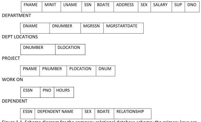
states satisfy the integrity constraints specified in IC. Figure 1.1 shows a relational database
schema
EMPLOYEE
FNAME MINIT LNAME SSN BDATE ADDRESS SEX SALARY SUP DNO
DEPARTMENT
DNAME DNUMBER MGRSSN MGRSTARTDATE
DEPT LOCATIONS
DNUMBER DLOCATION
PROJECT
PNAME PNUMBER PLOCATION DNUM
WORK ON
ESSN PNO HOURS
DEPENDENT
ESSN DEPENDENT NAME SEX BDATE RELATIONSHIP
Figure 1.1. Schema diagram for the company relational database schema; the primary keys are underlined.
1.2.3 Update Operations And Dealing With Constraint Violations
The operations of the relational model can be categorized into retrievals and updates. The
relational algebra operations, which can be use to specify retrievals, are discussed in details in a
later unit. In this unit, we concentrate on the update operations. There are three basic update
operations on relations (1) insert, (2) delete and (3) modify. Insert is used to insert a new tuple
or tuples in relation: Delete is used to delete tuple; and Update (or modify) is used to change
the values of some attribute in existing tuple. Whenever update operations are applied, the
integrity constraints specified on the relational database schema should not be violated. In this
unit we discuss the type of constraints that may be violated by each update operation and the
types of actions that may be taken if an update does cause a violation.
THE INSERT OPERATION
The insert operation provides a list of attribute values for a new tuple that is to be inserted into
unit. Domain constraints can be violated if an attribute value is given that does not appear in
the corresponding domain. Key constraints can be violating if a key value in the new tuple t
already exists in another tuple in the relation . Entity integrity can be violated if the primary
key of the new tuple t is null. Referential integrity can be violated if the value of any foreign key
in t refers to a tuple that does not exists in the referenced relation. Here are some example to
illustrate this discussion.
1. Insert < ‘Cecilia’, ‘F’, ‘Komolafe’, null, ‘1960‐04‐05’, ‘6357 Adetutu, Lane, Abeokuta, OG’,
F 28000, null 4> into EMPLOYEE. This insertion violates the entity integrity constraint
(null for the primary key SSN), so it is rejected.
2. Insert < ‘Alice’, ‘J’, ‘Zachariah’, ‘999887777’, ‘1960‐04‐05’, ‘6357 Adetutu Lane,
Abeokuta OG’, F,28000, ‘987654321’, 4> into EMPLOYEE. This insertion violates the key
constraint because another tuple with the same SSN value already exists in the
EMPLOYEE relation, and so it is rejected.
3. Insert < ‘Folorunso’, ‘O’,’Olusegun’,’677678989’, ‘1960‐04‐05’ ‘6357 Obasanjo Aremu
OG’, F,28000, ‘987654321’, 7 > into EMPLOYEE. This insertion violates the referential
integrity constraint specified on KNO because no DEPARTMENT tuples exists with
DNUMBERS = 7.
4. Insert < ‘Folorunso’, ‘O’, ‘Olusegun’, ‘677678989’, ‘1960‐04‐05’, ‘6357 Obasanjo Lane,
Aremu, OG’, F, 28000, null 4 > into EMPLOYEE. This insertion satisfies all constraints, so
it is acceptable.
If an insertion violates one or more constraints, the default option is to reject the insertion. In
this case, it would be useful if the DBMS could explain to the user why the insertion was
rejected. Another option is to attempt to correct the reason for rejecting the insertion, but this
is typically not used for violations caused by insert; rather, it is used more often in correcting
violations for Delete and Update. The following examples illustrate how this option may be
used for insert violations. In operation 1 above, the DBMS could ask the user to provide a value
for SSN and could accept the insertion if a valid SSN value was provided. In operation 3, the
DBMS could either, ask the user change the value of DNO to some valid values (or set it to null),
or it could ask the user to insert a DEPARTMENT tuple with DNUMBER =7 and could accept the
insertion only after such an operation was accepted. Notice that in the latter case the insertion
can cascade back to the EMPLOYEE relation if the user attempt to insert a tuple for department
7 with a value off MGRSS that does not exist in the EMPLOYEE relation.
THE DELETE OPERATION
The Delete operation can violate only referential integrity; If the foreign keys reference the
tuple being deleted from other tuples in the database. To specify deletion, a condition on the
attributes of the relation select the tuples (or tuples) to be deleted. Here are some examples.
1. Delete the WORKS‐ON tuples with ESS = 999887777 and KPNO = 10. This deletion is
acceptable.
2. Delete the employee tuple with SSN = 999887777. This deletion is not acceptable,
3. Delete the employee tuple with SSN = 333445555. This deletion will result in even worse
referential integrity violations, because the tuple involved is referenced by tuples from
the employee, department, works‐on, and department relations.
Three options are available if a deletion operation causes a violation,.
The first option is to reject the deletion.
The second opting is to attempt to cascade ( or propagate) the deletion by deleting
tuples that reference the tuple that is being deleted. For example in operation 2, the
DBMS could automatically delete the offending tuples form works‐on with ESSN=
999887777.
A third option is a to modify the referencing attribute that cause the valid tuple. Notice
that, if a referencing attribute that cause a violation is part of the primary key, it cannot
be set to null otherwise, it would violate entity integrity.
Combinations of these three options are also possible. For example, to avoid having operation 3
cause a violation, DBMS may automatically delete all tuples from works –on and department
with ESSN=333445555. Tuples in employee with super SSN = 33445555 and changed to other
valid values or to null. Although it may makes sense to delete automatically the works‐on and
department tuples that refer to an employee tuples, it may not make sense to delete other
employee tuples or a department tuple. In general, when a referential integrity constraint is
specified, the DBMS should allow the user to specify which of the three options applies in case
of a violation of the constraint.
THE UPDATE OPERATION
The update operation is used to change the values of one or more attributes in a tuple (or
tuples) of some relation r. It is necessary to specify a condition on the attribute of the relation
to select the tuple (or tuples) to be modified. Here are some examples.
1. Update the salary of the Employee tuple with SSN 999887777 to 28000 ‐ Acceptable
2. Update the DNO of the employee tuple with SSN = 999887777 to 1 ‐ Acceptable.
3. Update the DNO of the employee tuple with SSN = 999887777 to 7 ‐ Unacceptable,
because it violates referential integrity.
4. Update the SSN of the employee tuple with SSN = 999887777 to 987654321 ‐
Unacceptable, because it violates primary key and referential integrity constraints.
Updating an attribute that is neither a primary key nor a foreign key usually cause no problems.
The DBMS need only check to confirm that the new values as of the correct data type and
domain. Modifying a primary key value is similar to deleting one tuple and the issues discussed
earlier under both insert and delete comes into play. If a foreign key attribute is modified, the
DBMS must make sure that the new value refers to an existing tuple in the referenced relation
(or is null).
1.2.4 Basic Relational Algebra Operations
In addition to defining the database structure and constraints, a data model must include a set
of operations to manipulate the data. A basic set of relational model operations constitutes the
relational algebra. These operations enable the user to specify basic retrieval requests. The
result of a retrieval is a new relation, which may have been formed from one or more relations.
The algebra operations thus produce new relations, which can be further manipulated using
operations of the same algebra. A sequence of relational algebra operations forms a relation
algebra expression, whose result will also be a relation.
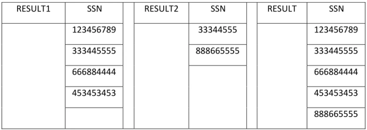
The relational algebra operations are usually divided into two groups. One group includes set
operations from mathematical set theory, these are applicable because each relation is defined
to be a set of tuples. Set operations include UNION, INTERSECTION, SET DIFFERENCE, and
CARTESIAN PRODUCT. The other group consists of operations developed specifically for
relational database; these include select , project, and join among others. The select and project
operations are discussed first, because they are the simplest, then we discuss set operations.
Finally, we discuss join and other complex operations. The relational database shown in Table
1.3 is used for our examples.
Some common database requests cannot be performed with the basic relational algebra
operations, so additional operations are needed to express these requests. Some of these
additional operations are described later.
THE SELECT OPERATIONS
The select operation is used to select a subset of the tuple from a relation that satisfy a
selection condition. One can consider the select operation to be a filter that keeps only those
tuples that satisfy a qualifying condition. For example, to select the employee tuples whose
departments is 4, or those whose salary is greater than N30,000, we can individually specify
each of these two conditions with a select operation as follows:
In general, the SELECT operation is denoted by
(sigma) is used to denote the SELECT operator, and the selection condition is a Boolean
expression specified on the attributes of relation
. Notice that
is generally a relational algebra expression whose result is a relation; the simplest expression is
just the name of database relation. The relation resulting from the select operations has the
same attributes as
. The Boolean expression specified in <selection condition> is made up of number of clauses of
the form
<attribute name> <comparison op><constant value>
or
<attribute name><comparison op><attribute name>
where <attribute name> is the name of an attribute of is normally one of the operators
{=<,>,e, and <constant value> is a constant value from the attribute domain. Clauses can be
arbitrarily connected by the Boolean operators AND OR and NOT or form a general selection.
For example, to select the tuples for all employees who either work in department 4 and make
over N25,000 per year, or work in department 5 and make over N30,0000 we can specify the
following select operation:
Table 1.3 Result of select and project operations.
(a)
FNAME MINT LNAME SSN BDATE ADD SEX SAL SUPERSSN DNO
Akin G Adeosun 123456789 1965‐01‐09 75 Fontren,
Housing OG F 5000 333445555 6
Ayo T Adeluola 33344555 1955‐12‐08 291,Itoko,
Abeokuta M 7000 88866555 5
Daniel O Olayinka 453453453 1972‐07‐31 34,Offmobil
Road M 3400 333445555 5
(b)
LNAME FNAME SALARY
Adeluola Ayo 70000
Olayinka Daniel 34000
Daunsi Jumoke 42000
Adjumo Kunle 50000
Bamidele Segun 40000
Oduntan Segun 45000
Olamide Kunle 80000
(c)
SEX SALARY
F 50000
M 70000
M 34000
F 42000
M 50000
M 40000
M 45000
M 80000
(a) (b) (c)
The result is shown in Table 1.5(a). Notice that the comparison operators in the set {=,<,>, }
apply to attribute whose domains are ordered values, such as numeric or date domains.
Domains of strings of characters are considered ordered based on the collating sequence of
the characters. If the domain of an attribute is a set of unordered values, then only the
comparison operations in the set {=””} can be used. An example of an unordered domain is the
domain colour = {red, blue, green, white, yellow} where no order is specified among the various
colours. Some domains allow additional types of comparison operations; for example, a domain
allows additional types of comparison operators. For example, a domain of character strings
In general the result of a SELECT operation can be determined as follows. The selection
condition is applied independently to each tuple
in
. this is done by substituting each occurrence of an attribute in the selection condition with its
value in the tuples . if the condition evaluates to true, then tuple
is selected. All the selected tuples appear in the result of the select operation. The Boolean
conditions AND, OR and NOT have their normal interpretation as follows:
(cond1 AND cond2 ) is true if both (cond1) and (cond2) are true. Otherwise, it is false
(cond1 OR cond2) is true if either (cond1) or (cond2) is true or both are true. Otherwise, it is
false.
(NOT cond) is true if cond is false. Otherwise, it is false.
The SELECT operator is unary, that is, it is applied to a single relation. Moreover, the selection
operation is applied to each tuple individually. Hence, selection conditions cannot involve more
than one tuple. The degree of the tuples in the resulting relation is always less than or equal to
the number to tuples in
. That is for any condition
. The fraction of tuples selected by a selection condition is referred to as the selectivity of the
conditions.
Notice that the select operation is commutative; that is,
Hence, a sequence of SELECTs can be allied in any order. In addition, we can always combine a
cascade of SELECT operations into a single SELECT operation with a conjunctive AND condition,
that is,
THE PROJECT OPERATION
If we think of a relation as a table, the SELECT operation selects some of the rows from the
table while discarding other rows. The PROJECT operation on the other hand, selects certain
attributes only. For example, to list each employees, first and last name and salary, we use the
PROJECT operation as follows:
LNAME, FNAME, SALARY (EMPLOYEE)
The result relation is shown in Table 1.3(b). The general form of the PROJECT operation is
<attribute list > (R)
Where (Pi) is the symbol used to represent the PROJECT operation and < attribute list> is a list
of attributes from the attributes of relation R. Again, notice that
is , in general, a relational algebra expression whose result is a relation, which in the simplest
case is just the name of a database relation. The result of the PROJECT operation has only the
attribute specified in attribute list and in the same order as they appear in the list. Hence, its
degree is equal to the number of attribute in attribute list. If the attribute list include only non
key attributes of
, duplicate tuple are likely to occur, the PROJECT operation removes any duplicate tuples. So
the result of the project operation is a set of tuples and hence a valid relation. This is known as
duplicate elimination. For example, consider the following PROJECT operation.
The result it shown in Table 1.3 (c). Notice that the tuple <F,25000> appears only once in TABLE
1.3(c) even though this combination of values appears twice in the employee relation.
The number of tuples in relation resulting from a PROJECT operations is always less than or
equal to the number of tuples in
. If the projection list is a superkey of that is, it includes some keys of R – the resulting
relation has the same number of tuples as R. Moreover as long as
contains the attribute in <list>. Otherwise, the left‐hand side is an incorrect expression.
It is also noteworthy that commutativity does not hold on PROJECT.
SEQUENCES OF OPERATIONS AND THE RENAME OPERATION
The relations shown in Table 1.3 do not have any names. In general, we may want to apply
several relational algebra operations one after the other. Either we can write the operations as
name, last name, and salary of all employee who work in department number 5, we must apply
a SELECT and a PROJECT operation. We can write a single relational algebra expression as
follows:
Table 1.4(a) shows the result of this relational algebra expression. Alternatively we can explicitly
show the sequence of operations, giving a name to each intermediate relation:
It is often simpler to break down a complex sequence of operations by specifying intermediate
result relations than to write a single relational algebra expression. We can also use this
technique to rename the attributes in the intermediate and result relations. This can be useful
in connection with more complex operations such as union and join as we shall see. To rename
the attributes in a relation, we simply list the new attribute names in parentheses, as in the
following example:
The two operations above are illustrated in figures 1.6(b). If no renaming is applied the names
of the attributes in the resulting relation of a SELECT operation are the same as those in the
original relation and in the same order. For a project OPERATION with no renaming, the
resulting relation has the same attribute names as those in the project list and in the same
order in which they appear in the list.
We can also define a RENAME operation which can rename either the relation name, or the
attribute name, or both in a manner similar to the way we defined select.
Table 1.3. Results of a relational algebra expression.
(a)
FNAME LNAME SALARY
Akin Adeosun 50000
Ayo Adeluola 70000
Jumoke Daunsi 42000
(b)
FNAME NINT LNAME SSN BDATE ADDRESS SEX SALARY SUPER DN
Akin G Adeosun 123456789 1965‐01‐09 75 F 50000 33445555 6
Ayo T Adeluola 3344555 1955‐12‐08 291,Itoko
Abeokuta M 70000 88866555 5
Daniel O Olayinka 453453453 1972‐07‐31 34 Off
Mobil Road M 34000 33445555 5
Jumoke O Daunsi 666884444 1964‐09‐15 23 Panseke
Street F 342000 333445555 5
(c)
FNAME LNAME SALARY
Akin Adeosun 50000
Ayo Adeluola 70000
Daniel Olayinka 34000
Jumoke Daunsi 42000
The same expression using intermediate relation and renaming of attribute and PROJECT. The
general RENAME operation when applied to a relation
of degree
is denoted by or . Where the symbol
(rho) is used to denote the rename operator,
is the new relation name, and are the new attribute names. The first expression rename
both the relation and its attributes; the second renames the relation only; and the third