TRANSMISSION MEDIA CHAPTER 4

(1)

C H A P T E R

4

T

RANSMISSION

M

EDIA

4.1 Guided Transmission Media Twisted Pair

Coaxial Cable Optical Fiber 4.2 Wireless Transmission

Antennas

Terrestrial Microwave Satellite Microwave Broadcast Radio Infrared

4.3 Wireless Propagation

Ground Wave Propagation Sky Wave Propagation Line-of-Sight Propagation 4.4 Line-of-Sight Transmission

Free Space Loss

Atmospheric Absorption Multipath

Refraction

4.5 Recommended Reading and Web Sites

4.6 Key Terms, Review Questions, and Problems Key Terms

Review Questions Problems

(2)

KEY POINTS

• The transmission media that are used to convey information can be classi-fied as guided or unguided. Guided media provide a physical path along which the signals are propagated; these include twisted pair, coaxial cable, and optical fiber. Unguided media employ an antenna for transmitting through air, vacuum, or water.

• Traditionally, twisted pair has been the workhorse for communications of all sorts. Higher data rates over longer distances can be achieved with coax-ial cable, and so coaxcoax-ial cable has often been used for high-speed local area network and for high-capacity long-distance trunk applications. However, the tremendous capacity of optical fiber has made that medium more attrac-tive than coaxial cable, and thus optical fiber has taken over much of the market for high-speed LANs and for long-distance applications.

• Unguided transmission techniques commonly used for information com-munications include broadcast radio, terrestrial microwave, and satellite. Infrared transmission is used in some LAN applications.

In a data transmission system, the transmission mediumis the physical path between transmitter and receiver. Recall from Chapter 3 that for guided media, electromag-netic waves are guided along a solid medium, such as copper twisted pair, copper coaxial cable, and optical fiber. For unguided media, wireless transmission occurs through the atmosphere, outer space, or water.

The characteristics and quality of a data transmission are determined both by the characteristics of the medium and the characteristics of the signal. In the case of guided media, the medium itself is more important in determining the limitations of transmission.

For unguided media, the bandwidth of the signal produced by the transmitting antenna is more important than the medium in determining transmission character-istics. One key property of signals transmitted by antenna is directionality. In gener-al, signals at lower frequencies are omnidirectional; that is, the signal propagates in all directions from the antenna. At higher frequencies, it is possible to focus the sig-nal into a directiosig-nal beam.

In considering the design of data transmission systems, key concerns are data rate and distance: the greater the data rate and distance the better. A number of de-sign factors relating to the transmission medium and the de-signal determine the data rate and distance:

• Bandwidth: All other factors remaining constant, the greater the bandwidth of a signal, the higher the data rate that can be achieved.

• Transmission impairments: Impairments, such as attenuation, limit the dis-tance. For guided media, twisted pair generally suffers more impairment than coaxial cable, which in turn suffers more than optical fiber.

• Interference: Interference from competing signals in overlapping frequency bands can distort or wipe out a signal. Interference is of particular concern for unguided media but is also a problem with guided media. For guided media,

(3)

4.1 / GUIDED TRANSMISSION MEDIA

95

102 Frequency

(Hertz) 103 ₁₀4 ₁₀5 ₁₀6 ₁₀7 ₁₀8 ₁₀9 ₁₀10 ₁₀11 ₁₀12 ₁₀13 ₁₀14 ₁₀15 Power and telephone

Rotating generators Musical instruments Voice microphones

Microwave

Radar

Microwave antennas Magnetrons

Infrared

Lasers Guided missiles Rangefinders

Radio

Radios and televisions Electronic tubes Integrated circuits

ELF VF

ELF Extremely low frequency VF Voice frequency VLF Very low frequency LF Low frequency

MF Medium frequency HF High frequency VHF Very high frequency

UHF Ultrahigh frequency SHF Superhigh frequency EHF Extremely high frequency

VLF LF MF HF VHF UHF SHF EHF

Twisted pair

Coaxial cable

Visible light

Optical fiber

FM radio and TV

AM radio Terrestrial and satellite transmission Wavelength

in space (meters)

106 ₁₀5 ₁₀4 ₁₀3 ₁₀2 ₁₀1 ₁₀0 ₁₀1 ₁₀2 ₁₀3 ₁₀4 ₁₀5 ₁₀6

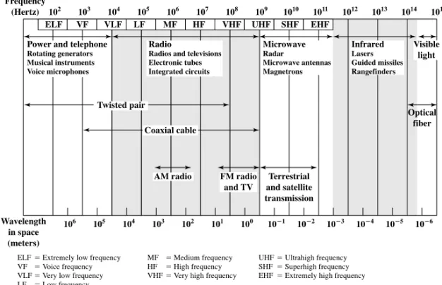
Figure 4.1 Electromagnetic Spectrum for Telecommunications

interference can be caused by emanations from nearby cables. For example, twisted pairs are often bundled together and conduits often carry multiple cables. Interference can also be experienced from unguided transmissions. Proper shielding of a guided medium can minimize this problem.

• Number of receivers: A guided medium can be used to construct a point-to-point link or a shared link with multiple attachments. In the latter case, each attachment introduces some attenuation and distortion on the line, limiting distance and/or data rate.

Figure 4.1 depicts the electromagnetic spectrum and indicates the frequencies at which various guided media and unguided transmission techniques operate. In this chapter we examine these guided and unguided alternatives. In all cases, we de-scribe the systems physically, briefly discuss applications, and summarize key trans-mission characteristics.

4.1 GUIDED TRANSMISSION MEDIA

For guided transmission media, the transmission capacity, in terms of either data rate or bandwidth, depends critically on the distance and on whether the medium is point-to-point or multipoint. Table 4.1 indicates the characteristics typical for the common guided media for long-distance point-to-point applications; we defer a dis-cussion of the use of these media for multipoint LANs to Part Four.

(4)

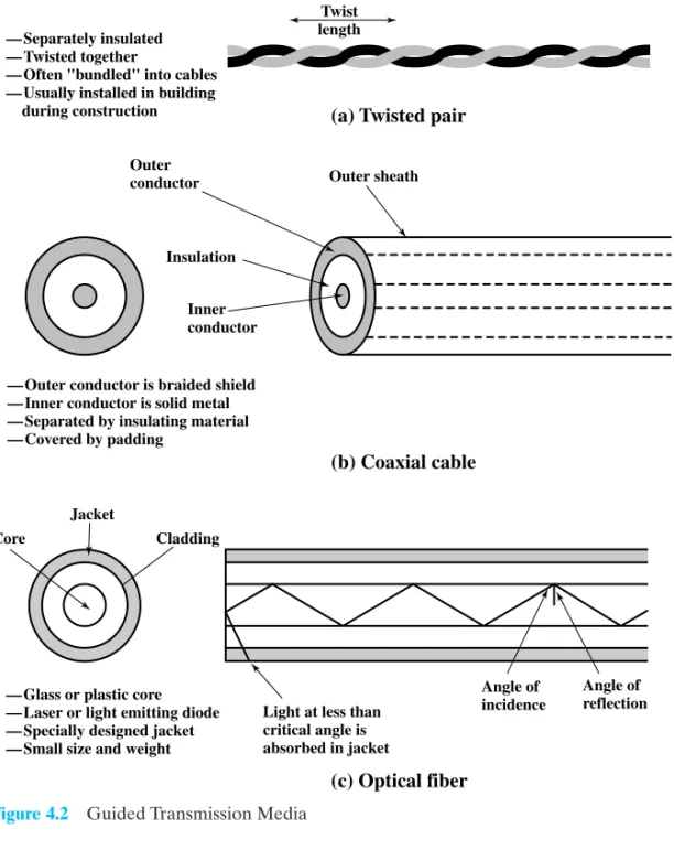
The three guided media commonly used for data transmission are twisted pair, coaxial cable, and optical fiber (Figure 4.2). We examine each of these in turn.

Twisted Pair

The least expensive and most widely used guided transmission medium is twisted pair. Physical Description

A twisted pair consists of two insulated copper wires arranged in a regular spi-ral pattern. A wire pair acts as a single communication link. Typically, a number of these pairs are bundled together into a cable by wrapping them in a tough protec-tive sheath. Over longer distances, cables may contain hundreds of pairs. The twist-ing tends to decrease the crosstalk interference between adjacent pairs in a cable. Neighboring pairs in a bundle typically have somewhat different twist lengths to re-duce the crosstalk interference. On long-distance links, the twist length typically varies from 5 to 15 cm. The wires in a pair have thicknesses of from 0.4 to 0.9 mm.

Applications

By far the most common transmission medium for both analog and digital sig-nals is twisted pair. It is the most commonly used medium in the telephone network and is the workhorse for communications within buildings.

In the telephone system, individual residential telephone sets are connected to the local telephone exchange, or “end office,” by twisted-pair wire. These are re-ferred to as subscriber loops. Within an office building, each telephone is also con-nected to a twisted pair, which goes to the in-house private branch exchange (PBX) system or to a Centrex facility at the end office. These twisted-pair installations were designed to support voice traffic using analog signaling. However, by means of a modem, these facilities can handle digital data traffic at modest data rates.

Twisted pair is also the most common medium used for digital signaling. For connections to a digital data switch or digital PBX within a building, a data rate of 64 kbps is common. Twisted pair is also commonly used within a building for local area networks supporting personal computers. Data rates for such products are typically in the neighborhood of 10 Mbps. However, twisted-pair networks with data rates of to 1 Gbps have been developed, although these are quite limited in terms of

Frequency Typical Typical Repeater Range Attenuation Delay Spacing

Twisted pair 0 to 3.5 kHz 2 km

(with loading)

Twisted pairs 0 to 1 MHz 2 km

(multi-pair cables)

Coaxial cable 0 to 500 MHz 1 to 9 km

Optical fiber 180 to 370 THz 0.2 to 0.5dB>km 5s>km 40 km 4s>km

7dB>km@10MHz

5s>km 3dB>km@1kHz

50s>km 0.2dB>km@1kHz

Table 4.1 Point-to-Point Transmission Characteristics of Guided Media [GLOV98]

(5)

97

(a) Twisted pair

(b) Coaxial cable

— Outer conductor is braided shield — Inner conductor is solid metal — Separated by insulating material — Covered by padding

Light at less than critical angle is absorbed in jacket

Angle of incidence

Angle of reflection Outer sheath

Insulation

Inner conductor

— Glass or plastic core — Laser or light emitting diode — Specially designed jacket — Small size and weight

(c) Optical fiber

Core

Jacket

Cladding

Twist length — Separately insulated

— Twisted together

— Often "bundled" into cables — Usually installed in building during construction

Outer conductor

Figure 4.2 Guided Transmission Media

the number of devices and geographic scope of the network. For long-distance ap-plications, twisted pair can be used at data rates of 4 Mbps or more.

Twisted pair is much less expensive than the other commonly used guided transmission media (coaxial cable, optical fiber) and is easier to work with.

Transmission Characteristics

Twisted pair may be used to transmit both analog and digital transmission. For analog signals, amplifiers are required about every 5 to 6 km. For digital transmis-sion (using either analog or digital signals), repeaters are required every 2 or 3 km. Compared to other commonly used guided transmission media (coaxial cable, optical fiber), twisted pair is limited in distance, bandwidth, and data rate. As

(6)

107 106 105 104 108 107 106

105 ₁₀12 ₁₀15

1 THz 109

1 GHz 103

1 kHz 10

6 1 MHz 103 102 Frequency (Hz) Attenuation (dB/km)

(a) Twisted pair (based on [REEV95]) 0 5 10 15 20 25 30 Attenuation (dB/km) 0 0.5 1.0 1.5 2.0 2.5 3.0

26-AWG (0.4 mm) 24-AWG (0.5 mm) 22-AWG (0.6 mm) 19-AWG (0.9 mm)

0.5 mm twisted pair

Frequency (Hz)

Attenuation

(dB/km)

(b) Coaxial cable (based on [BELL90]) 0 5 10 15 20 25 30 Attenuation (dB/km) 0 5 10 15 20 25 30

800 900 1000 1100 1200 1300 1400 1500 1600 1700 Wavelength in vacuum (nm)

(c) Optical fiber (based on [FREE02])

Frequency (Hz) (d) Composite graph

typical optical fiber 9.5 mm coax 3/8" cable (9.5 mm)

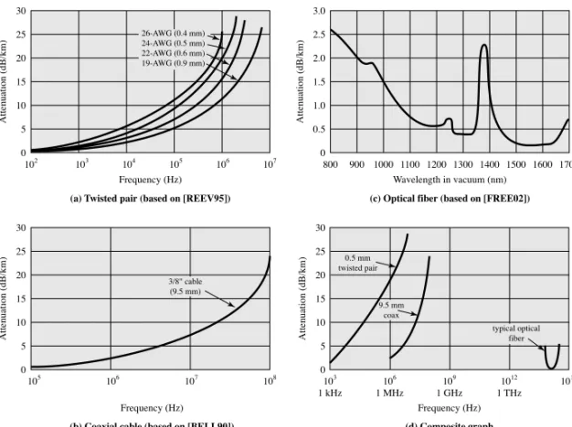
Figure 4.3 Attenuation of Typical Guided Media

Figure 4.3a shows, the attenuation for twisted pair is a very strong function of fre-quency. Other impairments are also severe for twisted pair. The medium is quite sus-ceptible to interference and noise because of its easy coupling with electromagnetic fields. For example, a wire run parallel to an ac power line will pick up 60-Hz energy. Impulse noise also easily intrudes into twisted pair. Several measures are taken to reduce impairments. Shielding the wire with metallic braid or sheathing reduces in-terference. The twisting of the wire reduces low-frequency interference, and the use of different twist lengths in adjacent pairs reduces crosstalk.

For point-to-point analog signaling, a bandwidth of up to about 1 MHz is pos-sible. This accommodates a number of voice channels. For long-distance digital point-to-point signaling, data rates of up to a few Mbps are possible; for very short distances, data rates of up to 1 Gbps have been achieved in commercially available products.

Unshielded and Shielded Twisted Pair

Twisted pair comes in two varieties: unshielded and shielded. Unshielded twisted pair (UTP) is ordinary telephone wire. Office buildings, by universal prac-tice, are prewired with excess unshielded twisted pair, more than is needed for sim-ple telephone support. This is the least expensive of all the transmission media commonly used for local area networks and is easy to work with and easy to install. Unshielded twisted pair is subject to external electromagnetic interference, in-cluding interference from nearby twisted pair and from noise generated in the

(7)

99

environment. A way to improve the characteristics of this medium is to shield the twisted pair with a metallic braid or sheathing that reduces interference. This shield-ed twistshield-ed pair (STP) provides better performance at higher data rates. However, it is more expensive and more difficult to work with than unshielded twisted pair.

Category 3 and Category 5 UTP

Most office buildings are prewired with a type of 100-ohm twisted pair cable commonly referred to as voice grade. Because voice-grade twisted pair is already in-stalled, it is an attractive alternative for use as a LAN medium. Unfortunately, the data rates and distances achievable with voice-grade twisted pair are limited.

In 1991, the Electronic Industries Association published standard EIA-568, Commercial Building Telecommunications Cabling Standard, which specifies the use of voice-grade unshielded twisted pair as well as shielded twisted pair for in-building data applications. At that time, the specification was felt to be adequate for the range of frequencies and data rates found in office environments. Up to that time, the prin-cipal interest for LAN designs was in the range of data rates from 1 Mbps to 16 Mbps. Subsequently, as users migrated to higher-performance workstations and applications, there was increasing interest in providing LANs that could operate up to 100 Mbps over inexpensive cable. In response to this need, EIA-568-A was issued in 1995. The new standard reflects advances in cable and connector design and test methods. It cov-ers 150-ohm shielded twisted pair and 100-ohm unshielded twisted pair.

EIA-568-A recognizes three categories of UTP cabling:

• Category 3: UTP cables and associated connecting hardware whose transmis-sion characteristics are specified up to 16 MHz

Of these, it is Category 3 and Category 5 cable that have received the most at-tention for LAN applications. Category 3 corresponds to the voice-grade cable found in abundance in most office buildings. Over limited distances, and with proper design, data rates of up to 16 Mbps should be achievable with Category 3. Category 5 is a data-grade cable that is becoming increasingly common for preinstallation in new office buildings. Over limited distances, and with proper design, data rates of up to 100 Mbps should be achievable with Category 5.

A key difference between Category 3 and Category 5 cable is the number of twists in the cable per unit distance. Category 5 is much more tightly twisted, with a typical twist length of 0.6 to 0.85 cm, compared to 7.5 to 10 cm for Category 3. The tighter twisting of Category 5 is more expensive but provides much better perfor-mance than Category 3.

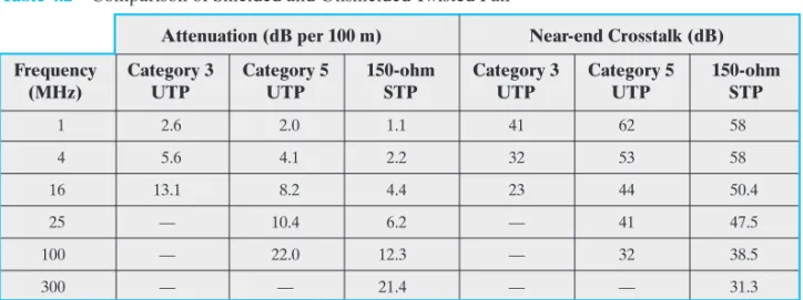
Table 4.2 summarizes the performance of Category 3 and 5 UTP, as well as the STP specified in EIA-568-A. The first parameter used for comparison, attenuation, is fairly straightforward. The strength of a signal falls off with distance over any transmission medium. For guided media attenuation is generally exponential and therefore is typically expressed as a constant number of decibels per unit distance.

(8)

Attenuation (dB per 100 m) Near-end Crosstalk (dB) Frequency Category 3 Category 5 150-ohm Category 3 Category 5 150-ohm

(MHz) UTP UTP STP UTP UTP STP

1 2.6 2.0 1.1 41 62 58

4 5.6 4.1 2.2 32 53 58

16 13.1 8.2 4.4 23 44 50.4

25 — 10.4 6.2 — 41 47.5

100 — 22.0 12.3 — 32 38.5

300 — — 21.4 — — 31.3

Table 4.2 Comparison of Shielded and Unshielded Twisted Pair

Table 4.3 Twisted Pair Categories and Classes

UTP Unshielded twisted pair FTP Foil twisted pair

SSTP =Shielded screen twisted pair

= =

Near-end crosstalk as it applies to twisted pair wiring systems is the coupling of the signal from one pair of conductors to another pair. These conductors may be the metal pins in a connector or wire pairs in a cable. The near end refers to coupling that takes place when the transmit signal entering the link couples back to the receiving conductor pair at that same end of the link (i.e., the near transmitted sig-nal is picked up by the near receive pair).

Since the publication of EIA-568-A, there has been ongoing work on the de-velopment of standards for premises cabling, driven by two issues. First, the Gigabit Ethernet specification requires the definition of parameters that are not specified completely in any published cabling standard. Second, there is a desire to specify ca-bling performance to higher levels, namely Enhanced Category 5 (Cat 5E), Catego-ry 6, and CategoCatego-ry 7. Tables 4.3 and 4.4 summarize these new cabling schemes and compare them to the existing standards.

Coaxial Cable

Physical Description

Coaxial cable, like twisted pair, consists of two conductors, but is constructed differently to permit it to operate over a wider range of frequencies. It consists of a hollow outer cylindrical conductor that surrounds a single inner wire conductor (Fig-ure 4.2b). The inner conductor is held in place by either regularly spaced insulating

Category 3 Category 5 Category 6 Category 7 Class C Class D Category 5E Class E Class F Bandwidth 16 MHz 100 MHz 100 MHz 200 MHz 600 MHz

Cable Type UTP UTP/FTP UTP/FTP UTP/FTP SSTP

Link Cost 0.7 1 1.2 1.5 2.2

(9)

101

Table 4.4 High-Performance LAN Copper Cabling Alternatives [JOHN98]

Name Construction Expected Performance Cost

Cable consists of 4 pairs of 24 AWG (0.50 mm) copper with thermoplastic polyolefin or fluorinated ethylene propylene (FEP) jacket. Outside sheath consists of polyvinylchlorides (PVC), a fire-retardant polyolefin or fluoropolymers.

Cable consists of 4 pairs of 24 AWG (0.50 mm) copper with thermoplastic polyolefin or fluorinated ethylene propylene (FEP) jacket. Outside sheath consists of polyvinylchlorides (PVC), a fire-retardant polyolefin or fluoropolymers. Higher care taken in design and manufacturing.

Cable consists of 4 pairs of 0.50 to 0.53 mm copper with thermoplastic polyolefin or fluorinated ethylene propylene (FEP) jacket. Outside sheath consists of polyvinylchlorides (PVC), a fire-retardant polyolefin or fluoropolymers. Extremely high care taken in design and manufacturing. Advanced connector designs. Cable consists of 4 pairs of 24 AWG (0.50 mm) copper with thermoplastic polyolefin or fluorinated ethylene propylene (FEP) jacket. Pairs are sur-rounded by a common metallic foil shield. Outside sheath consists of polyvinylchlorides (PVC), a fire-retardant polyolefin, or fluoropolymers. Cable consists of 4 pairs of 24 AWG (0.50 mm) copper with thermoplastic polyolefin or fluorinated ethylene propylene (FEP) jacket. Pairs are sur-rounded by a common metallic foil shield, followed by a braided metallic shield. Outside sheath consists of polyvinylchlorides (PVC), a fire-retardant polyolefin, or fluoropolymers. Also called PiMF (for Pairs in Metal Foil), SSTP of 4 pairs of 22-23AWG copper with a thermoplastic polyolefin or fluorinated ethylenepropylene (FEP) jacket. Pairs are individually sur-rounded by a helical or longitudinal metallic foil shield, followed by a braid-ed metallic shield. Outside sheath of polyvinylchlorides (PVC), a fire-retardant polyolefin, or fluoropolymers. Category 5 UTP

Enhanced Cat 5 UTP (Cat 5E)

Category 6 UTP

Foil Twisted Pair

Shielded Foil Twisted Pair

Category 7 Shielded-Screen Twisted Pair

Mixed and matched cables and con-necting hardware from various manu-facturers that have a reasonable chance of meeting TIA Cat 5 Chan-nel and ISO Class D requirements. No manufacturer’s warranty is involved.

Category 5 components from one sup-plier or from multiple supsup-pliers where components have been deliberately matched for improved impedance and balance. Offers ACR performance in excess of Cat 5 Channel and Class D as well as a 10-year or greater warranty.

Category 6 components from one sup-plier that are extremely well matched. Channel zero ACR point (effective bandwidth) is guaranteed to 200 MHz or beyond. Best available UTP. Perfor-mance specifications for Category 6 UTP to 250 MHz are under development.

Category 5 components from one sup-plier or from multiple supsup-pliers where components have been deliberately designed to minimize EMI susceptibil-ity and maximize EMI immunsusceptibil-ity. Vari-ous grades may offer increased ACR performance.

Category 5 components from one sup-plier or from multiple supsup-pliers where components have been deliberately designed to minimize EMI susceptibil-ity and maximize EMI immunsusceptibil-ity. Of-fers superior EMI protection to FTP.

Category 7 cabling provides positive ACR to 600 to 1200 MHz. Shielding on the individual pairs gives it phenomenal ACR.

ACR Attenuation to crosstalk ratio EMI =Electromagnetic interference

= 1 1.2 1.5 1.3 1.4 2.2

(10)

rings or a solid dielectric material. The outer conductor is covered with a jacket or shield. A single coaxial cable has a diameter of from 1 to 2.5 cm. Coaxial cable can be used over longer distances and support more stations on a shared line than twisted pair.

Applications

Coaxial cable is perhaps the most versatile transmission medium and is enjoy-ing widespread use in a wide variety of applications. The most important of these are

• Television distribution

• Long-distance telephone transmission • Short-run computer system links • Local area networks

Coaxial cable is widely used as a means of distributing TV signals to individual homes—cable TV. From its modest beginnings as Community Antenna Television (CATV), designed to provide service to remote areas, cable TV reaches almost as many homes and offices as the telephone. A cable TV system can carry dozens or even hundreds of TV channels at ranges up to a few tens of kilometers.

Coaxial cable has traditionally been an important part of the long-distance telephone network. Today, it faces increasing competition from optical fiber, terres-trial microwave, and satellite. Using frequency division multiplexing (FDM, see Chapter 8), a coaxial cable can carry over 10,000 voice channels simultaneously.

Coaxial cable is also commonly used for short-range connections between de-vices. Using digital signaling, coaxial cable can be used to provide high-speed I/O channels on computer systems.

Coaxial cable is used to transmit both analog and digital signals. As can be seen from Figure 4.3b, coaxial cable has frequency characteristics that are superior to those of twisted pair, and can hence be used effectively at higher frequencies and data rates. Because of its shielded, concentric construction, coaxial cable is much less susceptible to interference and crosstalk than twisted pair. The principal constraints on perfor-mance are attenuation, thermal noise, and intermodulation noise. The latter is present only when several channels (FDM) or frequency bands are in use on the cable.

For long-distance transmission of analog signals, amplifiers are needed every few kilometers, with closer spacing required if higher frequencies are used. The us-able spectrum for analog signaling extends to about 500 MHz. For digital signaling, repeaters are needed every kilometer or so, with closer spacing needed for higher data rates.

Optical Fiber

An optical fiber is a thin (2 to ), flexible medium capable of guiding an optical ray. Various glasses and plastics can be used to make optical fibers. The low-est losses have been obtained using fibers of ultrapure fused silica. Ultrapure fiber is

(11)

103

difficult to manufacture; higher-loss multicomponent glass fibers are more econom-ical and still provide good performance. Plastic fiber is even less costly and can be used for short-haul links, for which moderately high losses are acceptable.

An optical fiber cable has a cylindrical shape and consists of three concentric sections: the core, the cladding, and the jacket (Figure 4.2c). The coreis the inner-most section and consists of one or more very thin strands, or fibers, made of glass or plastic; the core has a diameter in the range of 8 to Each fiber is surround-ed by its own cladding, a glass or plastic coating that has optical properties different from those of the core. The interface between the core and cladding acts as a reflec-tor to confine light that would otherwise escape the core. The outermost layer, sur-rounding one or a bundle of cladded fibers, is the jacket. The jacket is composed of plastic and other material layered to protect against moisture, abrasion, crushing, and other environmental dangers.

Applications

One of the most significant technological breakthroughs in data transmission has been the development of practical fiber optic communications systems. Optical fiber already enjoys considerable use in long-distance telecommunications, and its use in military applications is growing. The continuing improvements in perfor-mance and decline in prices, together with the inherent advantages of optical fiber, have made it increasingly attractive for local area networking. The following charac-teristics distinguish optical fiber from twisted pair or coaxial cable:

• Greater capacity: The potential bandwidth, and hence data rate, of optical fiber is immense; data rates of hundreds of Gbps over tens of kilometers have been demonstrated. Compare this to the practical maximum of hundreds of Mbps over about 1 km for coaxial cable and just a few Mbps over 1 km or up to 100 Mbps to 1 Gbps over a few tens of meters for twisted pair.

• Smaller size and lighter weight: Optical fibers are considerably thinner than coaxial cable or bundled twisted-pair cable—at least an order of magnitude thinner for comparable information transmission capacity. For cramped con-duits in buildings and underground along public rights-of-way, the advantage of small size is considerable. The corresponding reduction in weight reduces structural support requirements.

• Lower attenuation: Attenuation is significantly lower for optical fiber than for coaxial cable or twisted pair (Figure 4.3c) and is constant over a wide range. • Electromagnetic isolation: Optical fiber systems are not affected by external

electromagnetic fields. Thus the system is not vulnerable to interference, impulse noise, or crosstalk. By the same token, fibers do not radiate energy, so there is little interference with other equipment and there is a high degree of security from eavesdropping. In addition, fiber is inherently difficult to tap. • Greater repeater spacing: Fewer repeaters mean lower cost and fewer sources

of error. The performance of optical fiber systems from this point of view has been steadily improving. Repeater spacing in the tens of kilometers for opti-cal fiber is common, and repeater spacings of hundreds of kilometers have been demonstrated. Coaxial and twisted-pair systems generally have repeaters every few kilometers.

(12)

Five basic categories of application have become important for optical fiber: • Long-haul trunks

• Metropolitan trunks • Rural exchange trunks • Subscriber loops • Local area networks

Long-haul fiber transmission is becoming increasingly common in the tele-phone network. Long-haul routes average about 1500 km in length and offer high capacity (typically 20,000 to 60,000 voice channels). These systems compete econom-ically with microwave and have so underpriced coaxial cable in many developed countries that coaxial cable is rapidly being phased out of the telephone network in such countries. Undersea optical fiber cables have also enjoyed increasing use.

Metropolitan trunking circuits have an average length of 12 km and may have as many as 100,000 voice channels in a trunk group. Most facilities are installed in underground conduits and are repeaterless, joining telephone exchanges in a metro-politan or city area. Included in this category are routes that link long-haul mi-crowave facilities that terminate at a city perimeter to the main telephone exchange building downtown.

Rural exchange trunks have circuit lengths ranging from 40 to 160 km and link towns and villages. In the United States, they often connect the exchanges of differ-ent telephone companies. Most of these systems have fewer than 5000 voice chan-nels. The technology used in these applications competes with microwave facilities. Subscriber loop circuits are fibers that run directly from the central exchange to a subscriber. These facilities are beginning to displace twisted pair and coaxial cable links as the telephone networks evolve into full-service networks capable of handling not only voice and data, but also image and video. The initial penetration of optical fiber in this application is for the business subscriber, but fiber transmis-sion into the home will soon begin to appear.

A final important application of optical fiber is for local area networks. Stan-dards have been developed and products introduced for optical fiber networks that have a total capacity of 100 Mbps to 10 Gbps and can support hundreds or even thousands of stations in a large office building or a complex of buildings.

The advantages of optical fiber over twisted pair and coaxial cable become more compelling as the demand for all types of information (voice, data, image, video) increases.

Optical fiber transmits a signal-encoded beam of light by means of total inter-nal reflection. Total internal reflection can occur in any transparent medium that has a higher index of refraction than the surrounding medium. In effect, the optical fiber acts as a waveguide for frequencies in the range of about to this cov-ers portions of the infrared and visible spectra.

Figure 4.4 shows the principle of optical fiber transmission. Light from a source enters the cylindrical glass or plastic core. Rays at shallow angles are reflect-ed and propagatreflect-ed along the fiber; other rays are absorbreflect-ed by the surrounding

1015Hertz; 1014

(13)

105

Input pulse Output pulse

(a) Step-index multimode

(c) Single mode

(b) Graded-index multimode

Figure 4.4 Optical Fiber Transmission Modes

material. This form of propagation is called step-index multimode, referring to the variety of angles that will reflect. With multimode transmission, multiple propaga-tion paths exist, each with a different path length and hence time to traverse the fiber. This causes signal elements (light pulses) to spread out in time, which limits the rate at which data can be accurately received. Put another way, the need to leave spacing between the pulses limits data rate. This type of fiber is best suited for trans-mission over very short distances. When the fiber core radius is reduced, fewer an-gles will reflect. By reducing the radius of the core to the order of a wavelength, only a single angle or mode can pass: the axial ray. This single-mode propagation pro-vides superior performance for the following reason. Because there is a single trans-mission path with single-mode transtrans-mission, the distortion found in multimode cannot occur. Single-mode is typically used for long-distance applications, including telephone and cable television. Finally, by varying the index of refraction of the core, a third type of transmission, known as graded-index multimode, is possible. This type is intermediate between the other two in characteristics. The higher re-fractive index (discussed subsequently) at the center makes the light rays moving down the axis advance more slowly than those near the cladding. Rather than zig-zagging off the cladding, light in the core curves helically because of the graded index, reducing its travel distance. The shortened path and higher speed allows light at the periphery to arrive at a receiver at about the same time as the straight rays in the core axis. Graded-index fibers are often used in local area networks.

Two different types of light source are used in fiber optic systems: the light-emitting diode (LED) and the injection laser diode (ILD). Both are semiconductor devices that emit a beam of light when a voltage is applied. The LED is less costly, operates over a greater temperature range, and has a longer operational life. The ILD, which operates on the laser principle, is more efficient and can sustain greater data rates.

(14)

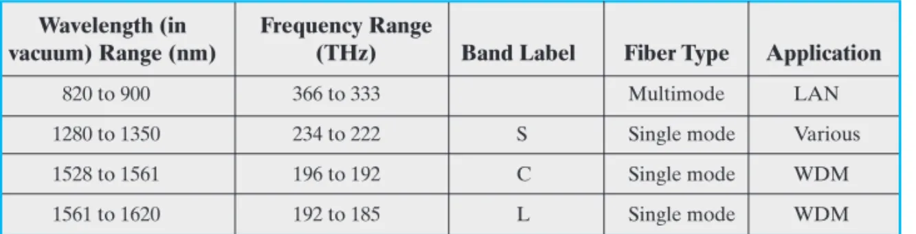
Wavelength (in Frequency Range

vacuum) Range (nm) (THz) Band Label Fiber Type Application

820 to 900 366 to 333 Multimode LAN 1280 to 1350 234 to 222 S Single mode Various 1528 to 1561 196 to 192 C Single mode WDM 1561 to 1620 192 to 185 L Single mode WDM Table 4.5 Frequency Utilization for Fiber Applications

WDM=wavelength division multiplexing (see Chapter 8)

There is a relationship among the wavelength employed, the type of transmis-sion, and the achievable data rate. Both single mode and multimode can support several different wavelengths of light and can employ laser or LED light sources. In optical fiber, based on the attenuation characteristics of the medium and on proper-ties of light sources and receivers, four transmission windows are appropriate, shown in Table 4.5.

Note the tremendous bandwidths available. For the four windows, the respec-tive bandwidths are 33 THz, 12 THz, 4 THz, and 7 THz. This is several orders of mag-nitude greater than the bandwidth available in the radio-frequency spectrum.

One confusing aspect of reported attenuation figures for fiber optic trans-mission is that, invariably, fiber optic performance is specified in terms of wave-length rather than frequency. The wavewave-lengths that appear in graphs and tables are the wavelengths corresponding to transmission in a vacuum. However, on the fiber, the velocity of propagation is less than the speed of light in a vacuum (c); the result is that although the frequency of the signal is unchanged, the wavelength is changed.

Example 4.1 For a wavelength in vacuum of 1550 nm, the corresponding fre-quency is

For a typical single mode fiber, the velocity of propagation is approximately In this case, a frequency of 193.4 THz corresponds to a

wave-length of Therefore, on

this fiber, when a wavelength of 1550 nm is cited, the actual wavelength on the fiber is 1055 nm.

The four transmission windows are in the infrared portion of the frequency spectrum, below the visible-light portion, which is 400 to 700 nm. The loss is lower at higher wavelengths, allowing greater data rates over longer distances. Many local applications today use 850-nm LED light sources. Although this combination is rel-atively inexpensive, it is generally limited to data rates under 100 Mbps and distances of a few kilometers. To achieve higher data rates and longer distances, a 1300-nm LED or laser source is needed. The highest data rates and longest distances require 1500-nm laser sources.

l = v>f = 12.04 * 1082>1193.4 * 10122 = 1055nm.

v = 2.04 * 108.

(15)

4.2 / WIRELESS TRANSMISSION

107

Figure 4.3c shows attenuation versus wavelength for a typical optical fiber. The unusual shape of the curve is due to the combination of a variety of factors that con-tribute to attenuation. The two most important of these are absorption and scatter-ing. In this context, the term scatteringrefers to the change in direction of light rays after they strike small particles or impurities in the medium.

4.2 WIRELESS TRANSMISSION

Three general ranges of frequencies are of interest in our discussion of wireless transmission. Frequencies in the range of about 1 GHz (gigahertz ) to 40 GHz are referred to as microwave frequencies. At these frequencies, highly di-rectional beams are possible, and microwave is quite suitable for point-to-point transmission. Microwave is also used for satellite communications. Frequencies in the range of 30 MHz to 1 GHz are suitable for omnidirectional applications. We refer to this range as the radiorange.

Another important frequency range, for local applications, is the infrared por-tion of the spectrum. This covers, roughly, from to Infrared is useful to local point-to-point and multipoint applications within confined areas, such as a single room.

For unguided media, transmission and reception are achieved by means of an antenna. Before looking at specific categories of wireless transmission, we provide a brief introduction to antennas.

Antennas

An antenna can be defined as an electrical conductor or system of conductors used either for radiating electromagnetic energy or for collecting electromagnetic ener-gy. For transmission of a signal, electrical energy from the transmitter is converted into electromagnetic energy by the antenna and radiated into the surrounding en-vironment (atmosphere, space, water). For reception of a signal, electromagnetic energy impinging on the antenna is converted into electrical energy and fed into the receiver.

In two-way communication, the same antenna can be and often is used for both transmission and reception. This is possible because any antenna transfers en-ergy from the surrounding environment to its input receiver terminals with the same efficiency that it transfers energy from the output transmitter terminals into the sur-rounding environment, assuming that the same frequency is used in both directions. Put another way, antenna characteristics are essentially the same whether an anten-na is sending or receiving electromagnetic energy.

An antenna will radiate power in all directions but, typically, does not per-form equally well in all directions. A common way to characterize the perper-formance of an antenna is the radiation pattern, which is a graphical representation of the ra-diation properties of an antenna as a function of space coordinates. The simplest pattern is produced by an idealized antenna known as the isotropic antenna. An

2 * 1014Hz.

3 * 1011

(16)

(a) Parabola y a

a b

b c

f f

c

x

Dir

ectrix

Focus

(b) Cross section of parabolic antenna showing reflective property

Figure 4.5 Parabolic Reflective Antenna

isotropic antennais a point in space that radiates power in all directions equally. The actual radiation pattern for the isotropic antenna is a sphere with the antenna at the center.

Parabolic Reflective Antenna

An important type of antenna is the parabolic reflective antenna, which is used in terrestrial microwave and satellite applications. You may recall from your precollege geometry studies that a parabola is the locus of all points equidistant from a fixed line and a fixed point not on the line. The fixed point is called the focus and the fixed line is called the directrix(Figure 4.5a). If a parabola is revolved about its axis, the surface generated is called a paraboloid. A cross section through the pa-raboloid parallel to its axis forms a parabola and a cross section perpendicular to the axis forms a circle. Such surfaces are used in headlights, optical and radio telescopes, and microwave antennas because of the following property: If a source of electro-magnetic energy (or sound) is placed at the focus of the paraboloid, and if the pa-raboloid is a reflecting surface, then the wave will bounce back in lines parallel to the axis of the paraboloid; Figure 4.5b shows this effect in cross section. In theory, this effect creates a parallel beam without dispersion. In practice, there will be some dispersion, because the source of energy must occupy more than one point. The larger the diameter of the antenna, the more tightly directional is the beam. On re-ception, if incoming waves are parallel to the axis of the reflecting paraboloid, the resulting signal will be concentrated at the focus.

(17)

109

Antenna Gain

Antenna gainis a measure of the directionality of an antenna. Antenna gain is defined as the power output, in a particular direction, compared to that produced in any direction by a perfect omnidirectional antenna (isotropic antenna). For exam-ple, if an antenna has a gain of 3 dB, that antenna improves upon the isotropic an-tenna in that direction by 3 dB, or a factor of 2. The increased power radiated in a given direction is at the expense of other directions. In effect, increased power is ra-diated in one direction by reducing the power rara-diated in other directions. It is im-portant to note that antenna gain does not refer to obtaining more output power than input power but rather to directionality.

A concept related to that of antenna gain is the effective areaof an antenna. The effective area of an antenna is related to the physical size of the antenna and to its shape. The relationship between antenna gain and effective area is

(4.1) where

antenna gain effective area carrier frequency speed of light carrier wavelength

For example, the effective area of an ideal isotropic antenna is with a power gain of 1; the effective area of a parabolic antenna with a face area of Ais 0.56A, with a power gain of

Example 4.2 For a parabolic reflective antenna with a diameter of 2 m, operating at 12 GHz, what is the effective area and the antenna gain? We have an area of and an effective area of The

wave-length is Then

Terrestrial Microwave

The most common type of microwave antenna is the parabolic “dish.” A typi-cal size is about 3 m in diameter. The antenna is fixed rigidly and focuses a narrow beam to achieve line-of-sight transmission to the receiving antenna. Microwave an-tennas are usually located at substantial heights above ground level to extend the range between antennas and to be able to transmit over intervening obstacles. To achieve long-distance transmission, a series of microwave relay towers is used, and point-to-point microwave links are strung together over the desired distance.

GdB = 45.46dB

G = 17A2>l2 = 17 * p2>10.02522 = 35,186

l = c>f = 13 * 1082>112 * 1092 = 0.025m.

Ae = 0.56p.

A = pr2 = p

7A>l2.

l2>4p,

l =

1L3 * 108m>s2

c =

f =

Ae =

G =

4pA_e

l2

=

4pf2Ae

(18)

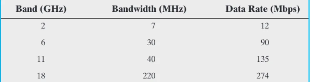
Band (GHz) Bandwidth (MHz) Data Rate (Mbps)

2 7 12

6 30 90

11 40 135

18 220 274

Table 4.6 Typical Digital Microwave Performance

Applications

The primary use for terrestrial microwave systems is in long haul telecommu-nications service, as an alternative to coaxial cable or optical fiber. The microwave facility requires far fewer amplifiers or repeaters than coaxial cable over the same distance but requires line-of-sight transmission. Microwave is commonly used for both voice and television transmission.

Another increasingly common use of microwave is for short point-to-point links between buildings. This can be used for closed-circuit TV or as a data link be-tween local area networks. Short-haul microwave can also be used for the so-called bypass application. A business can establish a microwave link to a long-distance telecommunications facility in the same city, bypassing the local telephone company. Another important use of microwave is in cellular systems, examined in Chapter 14.

Microwave transmission covers a substantial portion of the electromagnetic spectrum. Common frequencies used for transmission are in the range 1 to 40 GHz. The higher the frequency used, the higher the potential bandwidth and therefore the higher the potential data rate. Table 4.6 indicates bandwidth and data rate for some typical systems.

As with any transmission system, a main source of loss is attenuation. For mi-crowave (and radio frequencies), the loss can be expressed as

(4.2)

where dis the distance and is the wavelength, in the same units. Thus, loss varies as the square of the distance. In contrast, for twisted-pair and coaxial cable, loss varies exponentially with distance (linear in decibels). Thus repeaters or amplifiers may be placed farther apart for microwave systems—10 to 100 km is typical. Attenuation is increased with rainfall. The effects of rainfall become especially noticeable above 10 GHz. Another source of impairment is interference. With the growing popularity of microwave, transmission areas overlap and interference is always a danger. Thus the assignment of frequency bands is strictly regulated.

The most common bands for long-haul telecommunications are the 4-GHz to 6-GHz bands. With increasing congestion at these frequencies, the 11-GHz band is

l

L = 10loga

4pd

l b

2 dB

(19)

111

now coming into use. The 12-GHz band is used as a component of cable TV systems. Microwave links are used to provide TV signals to local CATV installations; the sig-nals are then distributed to individual subscribers via coaxial cable. Higher-frequency microwave is being used for short point-to-point links between buildings; typically, the 22-GHz band is used. The higher microwave frequencies are less useful for longer dis-tances because of increased attenuation but are quite adequate for shorter disdis-tances. In addition, at the higher frequencies, the antennas are smaller and cheaper.

Satellite Microwave

A communication satellite is, in effect, a microwave relay station. It is used to link two or more ground-based microwave transmitter/receivers, known as earth stations, or ground stations. The satellite receives transmissions on one frequency band (uplink), amplifies or repeats the signal, and transmits it on another frequency (downlink). A single orbiting satellite will operate on a number of frequency bands, called transponder channels, or simply transponders.

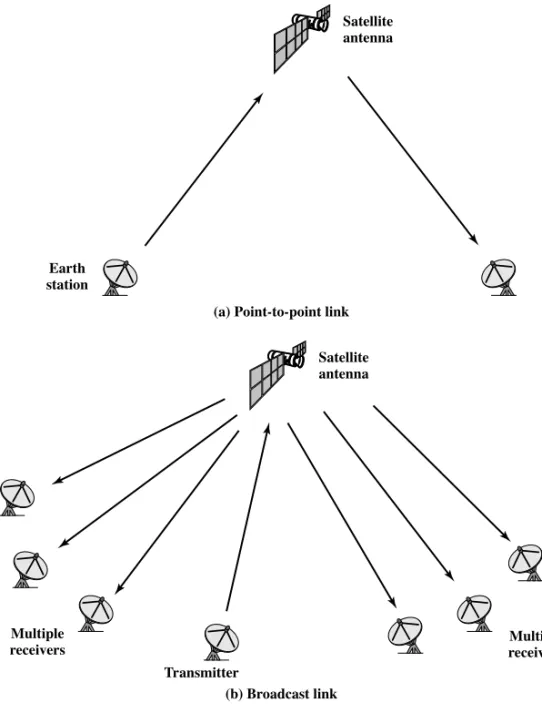
Figure 4.6 depicts in a general way two common configurations for satellite communication. In the first, the satellite is being used to provide a point-to-point link between two distant ground-based antennas. In the second, the satellite pro-vides communications between one ground-based transmitter and a number of ground-based receivers.

For a communication satellite to function effectively, it is generally required that it remain stationary with respect to its position over the earth. Otherwise, it would not be within the line of sight of its earth stations at all times. To remain sta-tionary, the satellite must have a period of rotation equal to the earth’s period of ro-tation. This match occurs at a height of 35,863 km at the equator.

Two satellites using the same frequency band, if close enough together, will in-terfere with each other. To avoid this, current standards require a spacing (angu-lar displacement as measured from the earth) in the 4/6-GHz band and a spacing at 12/14 GHz. Thus the number of possible satellites is quite limited.

Applications

The communication satellite is a technological revolution as important as fiber optics. Among the most important applications for satellites are the following:

• Television distribution

• Long-distance telephone transmission • Private business networks

Because of their broadcast nature, satellites are well suited to television distri-bution and are being used extensively in the United States and throughout the world for this purpose. In its traditional use, a network provides programming from a central location. Programs are transmitted to the satellite and then broadcast down to a number of stations, which then distribute the programs to individual

3° 4°

(20)

(a) Point-to-point link Satellite antenna

Earth station

(b) Broadcast link Transmitter

Multiple

receivers receiversMultiple

Satellite antenna

Figure 4.6 Satellite Communication Configurations

viewers. One network, the Public Broadcasting Service (PBS), distributes its televi-sion programming almost exclusively by the use of satellite channels. Other com-mercial networks also make substantial use of satellite, and cable television systems are receiving an ever-increasing proportion of their programming from satellites. The most recent application of satellite technology to television distribution is direct broadcast satellite (DBS), in which satellite video signals are transmitted di-rectly to the home user. The decreasing cost and size of receiving antennas have made DBS economically feasible, and a number of channels are either already in service or in the planning stage.

Satellite transmission is also used for point-to-point trunks between telephone exchange offices in public telephone networks. It is the optimum medium for

(21)

high-4.2 / WIRELESS TRANSMISSION

113

Ku-band satellite

Hub Server

PCs

Point-of-sale Terminals

Remote site

Remote site Remote

site

Figure 4.7 Typical VSAT Configuration

usage international trunks and is competitive with terrestrial systems for many long-distance intranational links.

Finally, there are a number of business data applications for satellite. The satel-lite provider can divide the total capacity into a number of channels and lease these channels to individual business users. A user equipped with the antennas at a num-ber of sites can use a satellite channel for a private network. Traditionally, such ap-plications have been quite expensive and limited to larger organizations with high-volume requirements. A recent development is the very small aperture termi-nal (VSAT) system, which provides a low-cost alternative. Figure 4.7 depicts a typi-cal VSAT configuration. A number of subscriber stations are equipped with low-cost VSAT antennas. Using some discipline, these stations share a satellite transmission capacity for transmission to a hub station. The hub station can exchange messages with each of the subscribers and can relay messages between subscribers.

The optimum frequency range for satellite transmission is in the range 1 to 10 GHz. Below 1 GHz, there is significant noise from natural sources, including galactic, solar, and atmospheric noise, and human-made interference from various electronic devices. Above 10 GHz, the signal is severely attenuated by atmospheric absorption and precipitation.

Most satellites providing point-to-point service today use a frequency band-width in the range 5.925 to 6.425 GHz for transmission from earth to satellite (up-link) and a bandwidth in the range 3.7 to 4.2 GHz for transmission from satellite to earth (downlink). This combination is referred to as the 4/6-GHz band. Note that the uplink and downlink frequencies differ. For continuous operation without interfer-ence, a satellite cannot transmit and receive on the same frequency. Thus signals re-ceived from a ground station on one frequency must be transmitted back on another.

(22)

The 4/6-GHz band is within the optimum zone of 1 to 10 GHz but has become saturated. Other frequencies in that range are unavailable because of sources of in-terference operating at those frequencies, usually terrestrial microwave. Therefore, the 12/14-GHz band has been developed (uplink: 14 to 14.5 GHz; downlink: 11.7 to 12.2 GHz). At this frequency band, attenuation problems must be overcome. How-ever, smaller and cheaper earth-station receivers can be used. It is anticipated that this band will also saturate, and use is projected for the 20/30-GHz band (uplink: 27.5 to 30.0 GHz; downlink: 17.7 to 20.2 GHz). This band experiences even greater attenuation problems but will allow greater bandwidth (2500 MHz versus 500 MHz) and even smaller and cheaper receivers.

Several properties of satellite communication should be noted. First, because of the long distances involved, there is a propagation delay of about a quarter sec-ond from transmission from one earth station to reception by another earth station. This delay is noticeable in ordinary telephone conversations. It also introduces problems in the areas of error control and flow control, which we discuss in later chapters. Second, satellite microwave is inherently a broadcast facility. Many sta-tions can transmit to the satellite, and a transmission from a satellite can be received by many stations.

Broadcast Radio

The principal difference between broadcast radio and microwave is that the former is omnidirectional and the latter is directional. Thus broadcast radio does not require dish-shaped antennas, and the antennas need not be rigidly mounted to a precise alignment.

Applications

Radiois a general term used to encompass frequencies in the range of 3 kHz to 300 GHz. We are using the informal term broadcast radioto cover the VHF and part of the UHF band: 30 MHz to 1 GHz. This range covers FM radio and UHF and VHF television. This range is also used for a number of data networking applications.

The range 30 MHz to 1 GHz is an effective one for broadcast communications. Unlike the case for lower-frequency electromagnetic waves, the ionosphere is trans-parent to radio waves above 30 MHz. Thus transmission is limited to the line of sight, and distant transmitters will not interfere with each other due to reflection from the atmosphere. Unlike the higher frequencies of the microwave region, broadcast radio waves are less sensitive to attenuation from rainfall.

As with microwave, the amount of attenuation due to distance obeys Equa-tion (4.2), namely Because of the longer wavelength, radio waves suffer relatively less attenuation.

A prime source of impairment for broadcast radio waves is multipath interfer-ence. Reflection from land, water, and natural or human-made objects can create

10loga4pd

l b

2 dB.

(23)

4.3 / WIRELESS PROPAGATION

115

multiple paths between antennas. This effect is frequently evident when TV recep-tion displays multiple images as an airplane passes by.

Infrared

Infrared communications is achieved using transmitters/receivers (transceivers) that modulate noncoherent infrared light. Transceivers must be within the line of sight of each other either directly or via reflection from a light-colored surface such as the ceiling of a room.

One important difference between infrared and microwave transmission is that the former does not penetrate walls. Thus the security and interference prob-lems encountered in microwave systems are not present. Furthermore, there is no frequency allocation issue with infrared, because no licensing is required.

4.3 WIRELESS PROPAGATION

A signal radiated from an antenna travels along one of three routes: ground wave, sky wave, or line of sight (LOS). Table 4.7 shows in which frequency range each pre-dominates. In this book, we are almost exclusively concerned with LOS communica-tion, but a short overview of each mode is given in this section.

Ground Wave Propagation

Ground wave propagation (Figure 4.8a) more or less follows the contour of the earth and can propagate considerable distances, well over the visual horizon. This effect is found in frequencies up to about 2 MHz. Several factors account for the tendency of electromagnetic wave in this frequency band to follow the earth’s cur-vature. One factor is that the electromagnetic wave induces a current in the earth’s surface, the result of which is to slow the wavefront near the earth, causing the wave-front to tilt downward and hence follow the earth’s curvature. Another factor is dif-fraction, which is a phenomenon having to do with the behavior of electromagnetic waves in the presence of obstacles.

Electromagnetic waves in this frequency range are scattered by the atmos-phere in such a way that they do not penetrate the upper atmosatmos-phere.

The best-known example of ground wave communication is AM radio.

Sky Wave Propagation

Sky wave propagation is used for amateur radio, CB radio, and international broad-casts such as BBC and Voice of America. With sky wave propagation, a signal from an earth-based antenna is reflected from the ionized layer of the upper atmosphere (ionosphere) back down to earth. Although it appears the wave is reflected from the ionosphere as if the ionosphere were a hard reflecting surface, the effect is in fact caused by refraction. Refraction is described subsequently.

A sky wave signal can travel through a number of hops, bouncing back and forth between the ionosphere and the earth’s surface (Figure 4.8b). With this propa-gation mode, a signal can be picked up thousands of kilometers from the transmitter.

(24)

116

F requency F ree-Space Band Range W av elength Range Propagation Characteristics T ypical Use

ELF (extremely low

30 to 300 Hz

10,000 to 1000 km

GW

P

ower line frequencies;

used by some home

frequenc

y)

control systems

VF (voice frequenc

y)

300 to 3000 Hz

1000 to 100 km

GW

Used by the telephone system for analog subscriber lines

VLF (very low

3 to 30 kHz

100 to 10 km

GW

;low attenuation day and night;

high

Long-range navigation;

submarine

frequenc

y)

atmospheric noise level

communication

LF (low frequenc

y)

30 to 300 kHz

10 to 1 km

GW

;slightly less reliable than

VLF;

Long-range navigation;

marine communication

absorption in daytime

radio beacons

MF (medium frequenc

y)

300 to 3000 kHz

1000 to 100 m

GW and night SW

;attenuation low at

Maritime radio;

direction finding;

night,

high in day;

atmospheric noise

AM broadcasting

HF (high frequenc

y)

3 to 30 MHz

100 to 10 m

S

W

;quality varies with time of day

, Amateur radio; international broadcasting , season, and frequenc y military communication; long-distance aircraft

and ship communication

VHF (very high

30 to 300 MHz

10 to 1 m

LOS;

scattering because of temperature

VHF television;

FM broadcast and two-way

frequenc

y)

inversion;

cosmic noise

radio

,AM aircraft communication;

aircraft

navigational aids

UHF (ultra high

300 to 3000 MHz

100 to 10 cm

LOS; cosmic noise UHF television; cellular telephone; radar; frequenc y) microwave links; personal communications systems

SHF (super high

3 to 30 GHz

10 to 1 cm

LOS;

rainfall attenuation above 10 GHz;

Satellite communication;

radar;

terrestrial

frequenc

y)

atmospheric attenuation due to oxygen

microwave links;

wireless local loop

and water vapor

EHF (extremely high

30 to 300 GHz

10 to 1 mm

LOS;

atmospheric attenuation due to

Experimental;

wireless local loop

frequenc

y)

oxygen and water vapor

Infrared

300 GHz to 400

THz

1 mm to 770 nm

LOS Infrared LANs; consumer electronic applications V isible light 400

THz to 900

THz

770 nm to 330 nm

LOS Optical communication T a ble 4.7 F requenc y Bands

(25)

4.3 / WIRELESS PROPAGATION

117

(b) Sky-wave propagation (2 to 30 MHz) (a) Ground-wave propagation (below 2 MHz)

Earth Transmit

antenna antennaReceive

Signal propagation

(c) Line-of-sight (LOS) propagation (above 30 MHz) Earth

Transmit

Signal propagation

Earth Ionospher

e

Transmit

Signal propagation

Figure 4.8 Wireless Propagation Modes

Line-of-Sight Propagation

Above 30 MHz, neither ground wave nor sky wave propagation modes operate, and communication must be by line of sight (Figure 4.8c). For satellite communication, a signal above 30 MHz is not reflected by the ionosphere and therefore a signal can be transmitted between an earth station and a satellite overhead that is not beyond the

(26)

1_{The exact value is 299,792,458 m/s.}

horizon. For ground-based communication, the transmitting and receiving antennas must be within an effectiveline of sight of each other. The term effectiveis used be-cause microwaves are bent or refracted by the atmosphere. The amount and even the direction of the bend depends on conditions, but generally microwaves are bent with the curvature of the earth and will therefore propagate farther than the optical line of sight.

Refraction

Before proceeding, a brief discussion of refraction is warranted. Refraction occurs because the velocity of an electromagnetic wave is a function of the density of the medi-um through which it travels. In a vacumedi-um, an electromagnetic wave (such as light or a radio wave) travels at approximately This is the constant, c, commonly re-ferred to as the speed of light, but actually referring to the speed of light in a vacuum.1In air, water, glass, and other transparent or partially transparent media, electromagnetic waves travel at speeds less than c.

When an electromagnetic wave moves from a medium of one density to a medi-um of another density, its speed changes. The effect is to cause a one-time bending of the direction of the wave at the boundary between the two media. Moving from a less dense to a more dense medium, the wave will bend toward the more dense medium. This phenomenon is easily observed by partially immersing a stick in water.

The index of refraction, or refractive index, of one medium relative to another is the sine of the angle of incidence divided by the sine of the angle of refraction. The index of refraction is also equal to the ratio of the respective velocities in the two media. The absolute index of refraction of a medium is calculated in comparison with that of a vacuum. Refractive index varies with wavelength, so that refractive ef-fects differ for signals with different wavelengths.

Although an abrupt, one-time change in direction occurs as a signal moves from one medium to another, a continuous, gradual bending of a signal will occur if it is moving through a medium in which the index of refraction gradually changes. Under normal propagation conditions, the refractive index of the atmosphere de-creases with height so that radio waves travel more slowly near the ground than at higher altitudes. The result is a slight bending of the radio waves toward the earth.

Optical and Radio Line of Sight

With no intervening obstacles, the optical line of sight can be expressed as:

where dis the distance between an antenna and the horizon in kilometers and his the antenna height in meters. The effective, or radio, line of sight to the horizon is ex-pressed as (Figure 4.9)

d = 3.572Kh

d = 3.572h

(27)

4.4 / LINE-OF-SIGHT TRANSMISSION

119 Earth

Optical horizon

Radio horizon

Antenna

Figure 4.9 Optical and Radio Horizons

where Kis an adjustment factor to account for the refraction. A good rule of thumb is Thus, the maximum distance between two antennas for LOS propaga-tion is where and are the heights of the two antennas.

Example 4.3 The maximum distance between two antennas for LOS trans-mission if one antenna is 100 m high and the other is at ground level is

Now suppose that the receiving antenna is 10 m high. To achieve the same dis-tance, how high must the transmitting antenna be? The result is

This is a savings of over 50 m in the height of the transmitting antenna. This ex-ample illustrates the benefit of raising receiving antennas above ground level to reduce the necessary height of the transmitter.

4.4 LINE-OF-SIGHT TRANSMISSION

Section 3.3 discussed various transmission impairments common to both guided and wireless transmission. In this section, we extend the discussion to examine some im-pairments specific to wireless line-of-sight transmission.

Free Space Loss

For any type of wireless communication the signal disperses with distance. There-fore, an antenna with a fixed area will receive less signal power the farther it is from the transmitting antenna. For satellite communication this is the primary mode of

h₁ = 7.842>1.33 = 46.2m

2Kh1 =

41

3.57 - 213.3 = 7.84 41 = 3.57

A

2Kh

1 + 213.3

B

d = 3.572Kh = 3.572133 = 41km

h₂ h₁ 3.57

A

2Kh₁ + 2Kh

2

B

, K = 4>3.

(28)

2_{As was mentioned in Appendix 3A, there is some inconsistency in the literature over the use of the}

terms gainand loss. Equation (4.3) follows the convention of Equation (2.2).

signal loss. Even if no other sources of attenuation or impairment are assumed, a transmitted signal attenuates over distance because the signal is being spread over a larger and larger area. This form of attenuation is known as free space loss, which can be express in terms of the ratio of the radiated power to the power received by the antenna or, in decibels, by taking 10 times the log of that ratio. For the ideal isotropic antenna, free space loss is

where

signal power at the transmitting antenna signal power at the receiving antenna carrier wavelength

propagation distance between antennas speed of light

where dand are in the same units (e.g., meters). This can be recast as

(4.3)

Figure 4.10 illustrates the free space loss equation.2

For other antennas, we must take into account the gain of the antenna, which yields the following free space loss equation:

where

gain of the transmitting antenna gain of the receiving antenna

effective area of the transmitting antenna effective area of the receiving antenna Ar =

At =

Gr =

Gt =

P_t Pr

= 1

4p221d22 G_r G

t l

2 =

1ld22

Ar At

= 1

cd22 f2_A

r A

t

= 20log

B 4pfd

c = 20log1f2 + 20log1d2 - 147.56dB LdB = 10log

Pt

Pr

= 20log

B 4pd

l = -20log1l2 + 20log1d2 + 21.98dB l

13 * 108m>s2

c =

d =

l =

Pr =

Pt =

Pt

Pr

= 1

4pd22

l2

= 1

4pfd22 c2

P_r P_t

(29)

4.4 / LINE-OF-SIGHT TRANSMISSION

121

60

1 5 10

Distance (km)

Loss

(dB)

f30 MHz

f300 MHz

f3 GHz

f30 GHz

f300 GHz

50 100

70 80 90 100 110 120 130 140 150 160 170 180

Figure 4.10 Free Space Loss

The third fraction is derived from the second fraction using the relationship between antenna gain and effective area defined in Equation (4.1). We can recast the loss equation as

(4.4)

Thus, for the same antenna dimensions and separation, the longer the carrier wave-length (lower the carrier frequency ), the higher is the free space path loss. It is in-teresting to compare Equations (4.3) and (4.4). Equation (4.3) indicates that as the frequency increases, the free space loss also increases, which would suggest that at higher frequencies, losses become more burdensome. However, Equation (4.4) shows that we can easily compensate for this increased loss with antenna gains.

f

= -20log1f2 + 20log1d2 - 10log1A_t Ar2 + 169.54dB LdB = 20log1l2 + 20log1d2 - 10log1A_t Ar2

(30)

In fact, there is a net gain at higher frequencies, other factors remaining constant. Equation (4.3) shows that at a fixed distance an increase in frequency results in an increased loss measured by However, if we take into account antenna gain, and fix antenna area, then the change in loss is measured by that is, there is actually a decrease in loss at higher frequencies.

Example 4.4 Determine the isotropic free space loss at 4 GHz for the short-est path to a synchronous satellite from earth (35,863 km). At 4 GHz, the

wave-length is Then,

Now consider the antenna gain of both the satellite- and ground-based antennas. Typical values are 44 dB and 48 dB, respectively. The free space loss is

Now assume a transmit power of 250 W at the earth station. What is the power received at the satellite antenna? A power of 250 W translates into 24 dBW, so the power at the receiving antenna is

Atmospheric Absorption

An additional loss between the transmitting and receiving antennas is atmospher-ic absorption. Water vapor and oxygen contribute most to attenuation. A peak at-tenuation occurs in the vicinity of 22 GHz due to water vapor. At frequencies below 15 GHz, the attenuation is less. The presence of oxygen results in an ab-sorption peak in the vicinity of 60 GHz but contributes less at frequencies below 30 GHz. Rain and fog (suspended water droplets) cause scattering of radio waves that results in attenuation. In this context, the term scatteringrefers to the produc-tion of waves of changed direcproduc-tion or frequency when radio waves encounter mat-ter. This can be a major cause of signal loss. Thus, in areas of significant precipitation, either path lengths have to be kept short or lower-frequency bands should be used.

Multipath

For wireless facilities where there is a relatively free choice of where antennas are to be located, they can be placed so that if there are no nearby interfering obstacles, there is a direct line-of-sight path from transmitter to receiver. This is generally the case for many satellite facilities and for point-to-point microwave. In other cases, such as mobile telephony, there are obstacles in abundance. The signal can be reflected by such obstacles so that multiple copies of the signal with varying delays

24 - 103.6 = -79.6dBW.

L_dB = 195.6 - 44 - 48 = 103.6dB

LdB = -20log10.0752 + 20log135.853 * 1062 + 21.98 = 195.6dB

13 * 1082>14 * 1092 = 0.075m.

-20log1f2;