An Implementation of Binomial Method of
Option Pricing using Parallel Computing
Sai K. Popuri?, Andrew M. Raim, Nagaraj K. Neerchal, Matthias K. Gobbert Department of Mathematics and Statistics, High Performance Computing Facility (HPCF) and Center forInterdisciplinary Research and Consulting (CIRC), University of Maryland, Baltimore County ?Contact author: [email protected]
Keywords: Option, Call, Put, Binomial Model, Bernoulli Path, Parallel Computing
Abstract
The Binomial method of option pricing is based on iterating over discounted option payoffs in a recursive fashion to calculate the present value of an option. Implementing the Binomial method to exploit the resources of a parallel computing cluster is non-trivial as the method is not easily parallelizable. We propose a procedure to transform the method into an “embarrass-ingly parallel” problem by mapping Binomial probabilities to Bernoulli paths. We have used the parallel computing capabilities inRwith theRmpipackage to implement the methodology on the cluster tara in the UMBC High Performance Computing Facility, which has 82 compute nodes with two quad-core Intel Nehalem processors and 24 GB of memory on a quad-data rate InfiniBand interconnect. With high-performance clusters and multi-core desktops becom-ing increasbecom-ingly accessible, we believe that our method will have practical appeal to financial trading firms.
1
Introduction
Options are a class of popular financial contracts that fall under the category of financial derivatives, which derive their value from a less complicated, often elementary asset called underlying, in addition to other factors. For this paper, it will suffice to think of a stock (e.g. Google trading on NASDAQ) as an asset. Financial derivatives are traded between two parties: a buyer and a seller. A buyer is the one who buys the financial derivative and a seller sells the contract.
An option is the right (but not an obligation) to buy or sell a certain number of shares at a prespecified fixed price within a prespecified time period. In other words, an option allows one to bet on the future movement of a stock. There are two types of options: call and put. A call (put) gives the buyer the right to buy (sell) a certain number of shares at a fixed price within a fixed time period. We denote the prespecified fixed price, called strike price, asK, and the time limit asT, which is also called time to maturity or expiration time. If the buyer of a call (put) decides to buy (sell) the shares at time t ≤ T, we say that the buyer has chosen to exercise the option. At time t ≤ T the buyer can also decide to sell the option itself. The buyer may also choose to not do anything until T, thereby letting the option expire. After T, an option is worthless. An option is called either an American or European depending on the time period during which it can be exercised. An American option can be exercised anytime beforeT. A European option, on the
other hand, can be exercised only at time T. Since an American option gives more flexibility to the buyer, it typically tends to be more expensive than its European counterpart.
The value of an option is the amount a seller (buyer) is willing to receive (pay) when the option is sold (bought). Valuation of an option is not a trivial problem to solve as the future movements of a stock are stochastic. Intuitively, for a call, the closer the current stock price is toK, the higher is the chance that it might exceed K at T, and therefore one would be willing to pay a higher value now to buy the call. Intuition also tells us that the call’s value must also depend on the time remaining before it expires as more time to maturity means higher probability of the stock exceeding K at T. Similar arguments can be made for a put. Therefore, the value of an option depends on two factors (in addition to others, which will be mentioned later): current stock price and time to maturity. There are several popular approaches that practitioners use to calculate the value, which is also called premium, of an option. We denote this value asV(St, t), where St is
the price of a stock at timet.
AlthoughV(St, t)fort < T is not known,V(ST, T), called payoff, is known with certainty at
T, whereST is the future price of the stock at the time of maturity. The valueV(ST, T)of a call
option at the time of maturityT is given by
V(ST, T) =
(
0 ifST ≤K ST −K ifST > K
= max{ST −K,0}. (1.1)
For a put option, the value at the time of maturityT is given by
V(ST, T) =
(
K−ST ifST < K
0 ifST ≥K
= max{K−ST,0}. (1.2)
Going back to the two factors mentioned earlier, stock price and time to maturity, the value of an option att < T therefore has two components: value associated with the stock price and value associated with the time to maturity. The first of these components is called intrinsic value and the second component is called time value. Clearly, as we get closer toT, much of the option’s value comes from its intrinsic value. This phenomenon is called the time decay of an option.
In addition to the strike priceK and time remaining to maturityT −t, the value of an option
V(St, t) also depends on the risk-free interest rate r and the volatility (standard derivation) σ of
the stock price. For simplicity, we assume that both r andσ stay constant during the life of the optionT −t. We also assume that the stock does not pay dividends during the life of the option. Dependence on r is motivated by the riskfree-hedging concept, which is related to building a portfolio of assets in such a way that its value grows at the rate offered by US Treasury bonds (since it is common practice to assume that US Treasury does not default on the bonds it issues, we consider the rate of return as riskfree). In this paper we will not go into the details of riskfree-hedging. We will also not discuss howσ of a stock is computed. Both the quantities are assumed to be given. Both rand σ are measured per year (time t is also measured in years). We assume that time starts att = 0, the time the option is to be bought or sold. Therefore, the range of time is
0 ≤t ≤T. To summarize, the value of a European option depends on the following five factors: expiration time (T), risk-free rate (r), volatility (σ), current stock price (St), and strike price (K).
In this paper we are concerned with a popular approach called Binomial method [2] or [5]. We will restrict our discussion to European options for simplicity.
Path-dependent options are a class of options whose payoff depends on the path the underlying takes until maturity. For example, the payoff of an Asian option depends on the average underlying price over the option’s lifetime. Our method could be attractive to value such path-dependent options, especially when the value is a complicated function of the paths.
The rest of the paper is organized as follows. Section 2 introduces the Binomial model and presents an algorithm to implement the method. In Section 3, we introduce the procedure to map Binomial probabilities to Bernoulli paths and present the formulation to value a European option using Bernoulli paths. Section 4 briefly discusses the implementation details on a parallel computing cluster. Section 5 presents results from the new procedure and finally, Section 6 gives some concluding remarks.
2
The Binomial Method
The Binomial method is based on simulating an evolution of the future stock price betweent = 0
andt = T on a grid of possible stock prices. An option’s value is calculated starting atT, using (1.1) for calls or (1.2) for puts, and stepping back in time by applying appropriate rules at each time step. Interested readers may refer to [2] or [5] for details.
Our goal is to calculate the value of an option at t = 0, i.e. V(St, t = 0). We first discretize
0≤t≤T into equidistant time steps of sizeδt. LetN be the number of time steps andδt=T /N. Let us denote points in time between0andT asti. Therefore,ti =iδtfori= 0, . . . , N. Imagine a two-dimensional grid withton the X-axis and stock priceSton the Y-axis; by discretizing time,
we slice the X-axis into equidistant time steps. As we describe below, we next discretizeStat each t=ti resulting in discrete valuesStij, wherejis the index on Y-axis. For notational convenience, we will writeStij asSij. The Binomial method makes the following assumptions:
A1 The stock priceSti atti over time stepδtcan only take two possible values: either go up to
Stiuor go down toStidatti+1 with0 < d < uwhereuis the factor of upward movement anddis the factor of downward movement.
A2 The probability of moving up between timeti andti+1 is p(and therefore the probability of
moving down is1−p). A3 E(Sti+1 |Sti) = Stie
rδt
The probability p does not reflect the true probability of a stock moving up. It is an artificial probability reflecting the assumption A3. From assumptions A1 and A2, we haveE(Sti+1 |Sti) =
pStiu+ (1−p)Stid. Equating this toE(Si+1 |Sti)in assumption A3 we get,
erδt=pu+ (1−p)d, (2.1)
and solving forp,
Algorithm 1Build the grid of stock prices and calculate option payoffs for Binomial method. fori= 1,2, . . . , N do
Sij =S0ujdi−j forj = 0,1, . . . , i
end for
forj = 0, . . . , N do
VN j ←max{SN j −K,0}
end for
Sincepis a probability,0≤p≤1implies thatd≤erδt≤u. Equating variances of the stock price process in the above discrete model and the continuous model (where stock price is assumed to be lognormally distributed), we get
e2rδt+σ2δt=pu2+ (1−p)d2. (2.3) To enforce symmetry in the simulated stock price structure, we assume
ud= 1. (2.4)
Solving (2.1), (2.3) and (2.4) we get
u=β+pβ2+ 1,
d= 1/u,
p= (erδt−d)/(u−d),
whereβ = 1 2(e
−rδt
+e(r+σ2)δt).
Starting with the current stock price in the marketS0, a grid of possible future stock pricesSij
is built using u, d and p. The procedure is shown as Algorithm 1. For a call option, the value
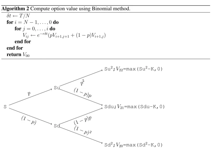
V(ST, T)is given using (1.1) at eachSN j atT. Therefore,VN j = max{SN j −K,0}, j = 0, .., N, where Vij represents V(Sij, ti). Figure 2.1 shows a two step Binomial tree which starts with a
stock priceS, and where the value for the last time step has been computed.
Now, to calculate the current value V00 = V(S0,0)of the option, a backward induction phase
recursively computes Vij for time steps ti = tN−1, tN−2, . . . , t0. The recursion is based on the
equation
Vij =e−rδt(pVi+1,j+1+ (1−p)Vi+1,j), (2.5)
which represents the expectation of the option value at stepi+ 1. The procedure to computeV00
is summarized as Algorithm 2.
3
Valuation using Bernoulli Paths
A careful look at Algorithm 2 reveals the difficulty in implementing the Binomial method in par-allel on a cluster. The method of backward induction uses option values computed in subsequent
Algorithm 2Compute option value using Binomial method.
δt←T /N
fori=N −1, . . . ,0do forj = 0, . . . , ido
Vij ←e−rδt(pVi+1,j+1+ (1−p)Vi+1,j)
end for end for returnV00
S
Sd Su
Sd2;V20=max(Sd2-K,0)
Sdu;V21=max(Sdu-K,0)
Su2;V22=max(Su2-K,0)
(1−
p) p
p2
(1−
p)p
(1−p)
p
(1−
p)2
Figure 2.1: A Two Step Binomial Tree
time steps, and implies that data be shared and communicated among the parallel tasks at each time step. If one were to parallelize the computation at each time step ti by grouping the
cal-culations into parallel tasks, it is clear that the results from the iteration forti+1 must be shared
across the tasks. This sharing of intermediary results at each iteration complicates the algorithm. Also, inter-task communication is generally orders of magnitude slower than calculation within a task, so the overall performance of a parallel implementation depends on making efficient use of the interconnect between compute nodes. The implementation can be greatly simplified and the communication cost can be removed if the problem is transformed into an “embarrassingly paral-lel problem”, which is defined as a problem in paralparal-lel computing that requires no communication among parallel tasks.
Several parallel implementation methods were proposed in recent years. Multi-threaded paral-lel implementations to price several options simultaneously on GPUs using the CUDA program-maing language were proposed by Kolb & Pharr [3]. Ganesan et al. [1] proposed another parallel implementation by concurrently processing multiple time steps using a symbolic dependence struc-ture. To the best of our knowledge, none of these procedures have taken the approach of making the Binomial method embarrassingly parallel. We propose a method to price European style options by mapping Binomial probabilities to Bernoulli asset paths, thereby transforming the Binomial
method into an embarrassingly parallel problem readily amenable for implementation on a parallel computing cluster.
Consider the backward induction step (2.5) in the Binomial method
Vij ←e−rδt(pVi+1,j+1+ (1−p)Vi+1,j)
for the two step tree shown in Figure 2.1. V22,V21, andV20are payoffs atT = 2. AtT = 1, option
values are computed as
V10=e−rδt(pV21+ (1−p)V20) (3.1)
and
V11=e−rδt(pV22+ (1−p)V21) (3.2)
AtT = 0, the option value is computed as
V00=e−rδt(pV11+ (1−p)V10) (3.3)
Substituting (3.1) and (3.2) in (3.3) yields
V00 =V01=e−rT(p2V22+ 2p(1−p)V21+ (1−p)2V20)
Note thatp2 = 20p2,2p(1−p) = 21p(1−p), and(1−p)2 = 22(1−p)2. Generalizing toN
time steps, the option valueV00can be calculated as
V00=e−rT
N
X
i=0
N i
pi(1−p)N−iVN i.
In vector form,V00can be represented as
V00=e−rTP0V, (3.4)
whereP is an(N+ 1)dimensional vector of probabilities andV is an(N+ 1)dimensional vector of payoffs at timet = T. All vectors are assumed to be column vectors. Each elementPi in the
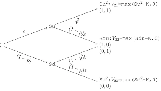
vectorP represents the probability of reaching the ithnode at timet = T, which can be reached in Niways through sequences of ups and downs, whereiis from 0toN withi= 0representing the leaf node reached after all down moves. We represent each such path by an N dimensional vector whose elements take either 1(up) or 0(down) as values. For example, x = (1,1, . . . ,1)0
represents a path of N up moves reaching the top most node at time t = T. Figure 3.1 shows the two step Binomial tree from Figure 2.1 with Bernoulli paths to terminal leaf nodes shown as vectors.
The probability of reaching a leaf node via the pathxis given by
P(X =x) =px01(1−p)N−x01 (3.5) where1is a vectorN ones. Since there are Niways of reaching the leaf nodei,
Pi =
N i
pi(1−p)N−i = X
x∈BN:x01=i
S
Sd Su
Sd2;V23=max(Sd2-K,0)
(0,0)
Sdu;V22=max(Sdu-K,0)
(1,0) (0,1)
Su2;V21=max(Su2-K,0)
(1,1)
(1−
p) p
p2
(1−
p)p
(1−p)
p
(1−
p)2
Figure 3.1: Two Step Binomial Tree with Bernoulli Paths
whereB={0,1}. Using (3.6) in (3.4) and after expanding the inner product, we obtain that
V00=e−rT
N
X
i=0
VN i
X
x∈BN:x01=i
px01(1−p)N−x01 (3.7)
Observe that by transforming the backward induction procedure into an expected option value at timeT as a summation over payoffs from each Bernoulli path, the problem becomes embarrass-ingly parallel.
4
Parallel Bernoulli Path Algorithm
Since the components of the summation in (3.7) are independent of each other, the calculation of the summation can be easily delegated to a set of processors (i.e. cores for multi-core CPUs) on a cluster. LetM be the number of parallel tasks, which is equal to the number of processors we intend to use on a cluster. A compute node for our discussion contains either single or a multiple processors. It is assumed that compute nodes may communicate by an interconnect. We use a master-worker paradigm for our implementation. The master first builds the lattice and calculates the option payoffVN j (although workers can compute their own payoffs once paths are delegated
to them), wherej = 0, .., N, at timeT. Note that ifN is the number of time steps used to build a lattice, the total number of paths leading to terminal payoffs is2N. It then divides these2N paths
into M sets with each set containing b2N/Mc number of paths. Paths remaining, if any, after
grouping are added to the last set. LetBm be themthset ofb2N/Mcpaths leading toKmdistinct payoffs. LetPm be a vector of dimensionKm with each elementPmi representing the probability
of reaching theithterminal payoff,i= 1, . . . , K
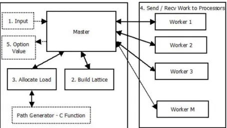
Figure 4.1: Program Structure
in 3. Assuming no payoff is assigned to more than one parallel task, note thatP0can be partitioned as
P10 P20 · · · PM0
. The master then sends each such setBmalong with their payoffsVNm, Pm,
interest rater, and time to maturityT to themthworker compute node. VNm represents a vector of payoffs from the paths inBm.
Themthparallel task evaluates the expected value of the option ase−rTP0
mVNm and returns it
to the master. Once the computed components of the option value are received from all workers, the final option value is computed by summing the individual components. A schematic depiction of the algorithm is presented in Figure 4.1. All the parameters needed to build the lattice and to evaluate the value of the option are provided to the master as input. The master then builds the lattice, allocates the load by calculating all the Bernoulli paths (generation of all such paths is not discussed in this paper) to the payoffs and grouping these paths into M sets. It then distributes these sets toM workers, which calculate and return the discounted expected values of the payoffs assigned to them. The master then calculates the option value by summing the values returned. Note that the workers do not need to communicate with each other once the master delegates the computation. The ease and simplicity in the implementation is a result of making the problem embarrassingly parallel. Figures 4.2 and 4.3 show code snippets inRfor master and worker tasks respectively.
5
Results
We have tested the implementation on the cluster tara in the UMBC High Performance Computing Facility, which has 82 computing nodes with two quad-core Intel Nehalem processors (therefore 8 cores per compute node) and 24 GB of memory on a quad-data rate InfiniBand interconnect, and have usedR[4, 6] as the programming environment.
We take a European put as an example to illustrate our results. The put has a strike price of
mpi.spawn.Rslaves(nslaves=M,needlog=FALSE) mpi.bcast.cmd(source("Worker.R"))
mpi.bcast.cmd(slave())
mpi.bcast(as.integer(N),type=1,rank=0) .
.
for(i in 1:length(W)) {
mpi.send.Robj(W[[i]],dest=i,tag=88,comm=1) }
atag <- mpi.any.tag()
asource <- mpi.any.source() for(nm in 1:length(W)) {
retsl <- mpi.recv.Robj(source=asource,tag=atag,comm=1) optval <- optval + retsl[2]
}
Figure 4.2: Rmpi code for master N <- mpi.bcast(integer(1),type=1,rank=0,comm=1) P <- mpi.bcast.Robj(rank=0,comm=1)
V <- mpi.recv.Robj(tag=88,source=0,comm=1) .
.
myrank <- mpi.comm.rank() retwkr <- c(myrank,sumtotal)
mpi.send.Robj(retwkr,dest=0,tag=2)
Figure 4.3: Rmpi code for worker rate is6%and time to maturity is one year.
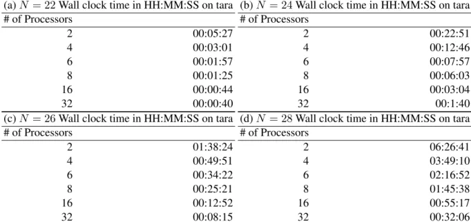
Table 5.1 shows the runtime for number of time stepsN = 22,N = 24,N = 26, andN = 28. Although the runtime drastically decreases as the number of parallel tasks increase for a given number of time steps, the scale of runtime itself also increases sharply as the number of time steps increase. This behavior suggests that the Bernoulli path procedure might be more suitable to price a certain class of complicated exotic options, possibly illiquid, that do not require large number of time steps in a lattice setting.
Figure 5.1 (a) shows the convergence rate of our method to the analytical solution (as the number of time stepsN increases), which is available for European options. Figure 5.1 (b) shows speedup rates as the number of parallel processes increase. IfTp(N)denotes the wall clock time
for a problem of a fixed size parametrized by N using p processes, then the quantity Sp(N) = T1(N)/Tp(N) measures the speedup of the code from 1 to pprocesses, whose optimal value is Sp =p. Note that for a fixed problem size, there is a reduced advantage in the speedup beyond a
Table 5.1: Runtime for different number of time steps
(a)N = 22Wall clock time in HH:MM:SS on tara # of Processors
2 00:05:27
4 00:03:01
6 00:01:57
8 00:01:25
16 00:00:44
32 00:00:40
(b)N = 24Wall clock time in HH:MM:SS on tara # of Processors
2 00:22:51
4 00:12:46
6 00:07:57
8 00:06:03
16 00:03:04
32 00:1:40
(c)N = 26Wall clock time in HH:MM:SS on tara # of Processors
2 01:38:24
4 00:49:51
6 00:34:22
8 00:25:21
16 00:12:52
32 00:08:15
(d)N = 28Wall clock time in HH:MM:SS on tara # of Processors
2 06:26:41
4 03:49:10
6 02:16:52
8 01:45:38
16 00:55:17
32 00:32:06
(a) (b)
Figure 5.1: (a) Convergence to analytical solution and (b) Speedup rate
time spent doing useful calculations. This issue is commonly encountered in parallel computing, and further discussion is beyond the scope of this paper.
6
Concluding Remarks
We have discussed a novel procedure to implement the Binomial method of option pricing in a parallel computing framework by mapping the Binomial probabilities of stock price evolution to Bernoulli paths, thereby transforming the problem into an embarrassingly parallel problem. The valuation based on our method is consistent with the value calculated by the traditional Binomial method. We have provided the outline of anRbased implementation using theRmpipackage on a cluster, which can be as small as a multi-core laptop with necessary parallel computing infras-tructure installed. In the future, we plan to evaluate our method in comparison with some of the known numerical methods to value path-dependent options.
Acknowledgments
The hardware used in the computational studies is part of the UMBC High Performance Computing Facility (HPCF). The facility is supported by the U.S. National Science Foundation through the MRI program (grant no. CNS–0821258) and the SCREMS program (grant no. DMS–0821311), with additional substantial support from the University of Maryland, Baltimore County (UMBC). Seewww.umbc.edu/hpcffor more information on HPCF and the projects using its resources. Financial support for this project is from HPCF and Department of Mathematics and Statistics at UMBC.
References
[1] Narayan Ganesan, Roger D. Chamberlain, and Jeremy Buhler. Acceleration of binomial op-tions pricing via parallelizing along time-axis on a GPU.Proc. of Symp. on Application Accel-erators in High Performance Computing, 2009.
[2] John C. Hull. Options, Futures, And Other Derivatives. Prentice Hall, 2000.
[3] C. Kolb and M. Pharr. Option pricing on the GPU in GPU Gems 2. Addison-Wesley, 2005.
[4] R Core Team. R: A Language and Environment for Statistical Computing. R Foundation for Statistical Computing, Vienna, Austria, 2012. ISBN 3-900051-07-0.
[5] R¨udiger Seydel. Tools for Computational Finance. Springer, 2003.
[6] Hao Yu. Rmpi documentation. http://cran.r-project.org/web/packages/ Rmpi.
![(Z) 1 Chloro 1 [2 (2 nitrophenyl)hydrazinylidene]propan 2 one](data:image/gif;base64,R0lGODlhAQABAIAAAP///wAAACH5BAEAAAAALAAAAAABAAEAAAICRAEAOw==)