Object-Relational Query Processing
Johan Petrini
Department of Information Technology
Uppsala University, Sweden
[email protected]
1. Introduction
In the beginning, there where flat files of data with no querying capabilities. Then came the relational database, RDBMS, with data structured according to some schema, and a standardized query language, SQL.
As time went by and with the growing need for people to store and model more complex data such as e.g. multi-media data, the relational database had to be extended with support for customized data types, functions and indexes. Databases with such capabilities were called object relational databases or ORDBMS. An extension to the SQL standard, SQL-99 (a subset of SQL3 [2]), was also needed to reflect these new capabilities and allow the user to utilize them in a declarative manor.
However, adding new functionality to the relational database also implicated rebuilding the traditional relational database optimizer to handle this new functionality and keep on creating scalable execution plans. Basically, all information hard-coded in the RDBMS about fixed data types should be replaced with a table-driven system supporting e.g. user defined types, functions and indexes, to be efficiently handled by the optimizer [1]. In particular, a new more advanced cost-function must also be developed for the optimization of query plans containing calls to expensive user defined functions.
2. Object-relational database
systems
Object relational query processing is needed to speed up queries over object-relational
databases. Before discussing the object-relational optimizer in section 3 we here
describe a couple of features mentioned in [1] to characterize an ORDBMS. These features are needed to model real-world problems in a way that is intuitive and easy for the developer and also offers good performance for the
application.
First, the DBMS should offer support for creating user defined base data types. The DBMS should also be possible to define functions and operators over the user defined base data types.
Second, the DBMS should offer support for creation of complex objects. A complex object is an object that can be constructed from multiple user defined base data types using some type constructor e.g. row, set or reference (OID). References are used to model primary key foreign key relationships [2].
Third, inheritance for user defined data types and functions (overloading) should be supported by the DBMS.
3. Object relational query
processing
There are several features of an ORDBMS that has to be properly handled by the
object-relational query optimizer [1]. Here, we will discuss a few of them and illustrate how they should be supported by the object relational optimizer using the examples from [1]. An example from [3] will also be introduced. The running example in the text will be the table
emp created to hold instances of the row type
employee_t as shown below:
create row type employee_t(
id employee_id, name varchar(30), salary int,
startdate date, location point, picture image); create table emp of type employee_t;
The user-defined type point above is created to model points in 2-D in a more simple way than adding the two attributes longitude and latitude as floating point numbers.
3.1 User-defined operators and selectivity functions
As opposed to relational databases where the selectivity functions for built-in operators is hard-coded into the system this knowledge has to be explicitly defined for user defined
operators in ORDBMS for the optimizer to do a good job.
For example, given the query below containing a call to the user -defined operator,
N_equator_equals, the user must also specify a corresponding selectivity function for the function:
select name from emp where
location N_equator_equals point(‘500,1’);
In the ORDBMS there should be functionality to associate this user-defined selectivity function to the operator. During optimization
time when the optimizer encounters the call to
N_equator_equals it will call the correct selectivity function and use the returned value (floating-point number between 0-1) to get a measurement of the cardinality of the user-defined function. Often the selectivity function use statistics from the ORDBMS to calculate its value.
3.2 User-defined access methods An access method is a collection of functions for handling indexes on data such as open a scan of an index, iterate through the scan, insert, delete or replace a record and close the scan. Consider the query below extracting the employees that lives within the area defined as the bounding box specified by origin and
point(1,1):
select name from emp where
location contained box(‘0,0,1,1’);
Since finding all the point contained within the bounding box is a 2-dimensional search there is a need for a 2-dimensional index such as e.g. an R-tree. A plain B-tree will not do. Since an ORDBMS allows the creation of user-defined types, e.g. point, special access methods are needed to speed up access to data defined in terms of these types. However, different data types using the same index in their access methods can assign different semantics to the operators (<,>,= e.t.c) of the particular index. The optimizer must be made aware of these characteristics to be able to do a good job optimizing the query. Therefore, a template has to be defined for every index specifying the operators of the index. Then when a new access method is added the user should specify which interpretation of the index operators that should be associated with the access method. With this information the optimizer has enough
Also, the access method must handle tasks like locking on index objects, recovery of index data structures and coordination with the ORDBMS buffer manager when reading and writing index disk pages.
3.3 Expensive clauses and functions The ability of the optimizer to find the correct placement of expensive clauses/functions in the query plan can have an enormous impact on the query processing time. Consider the query below extracting the name of employees with a salary over 10000 and low redness in their pictures:
1. select name 2. from emp 3. where
4. redness (picure) < 0.1 and 5. salary > 10000;
We assume that the clause on line 4 requires 100 CPU instructions to be evaluated while the clause on line 5 needs about 1000000 times as many instructions. We also assume for now that there are no indexes on the emp table.
In a relational DBMS the optimizer would have chosen to perform a sequential scan and evaluated the predicates for each extracted record from left to right. This is not a poor strategy since in traditional SQL clauses are often cheap w.r.t. CPU time. In the case with expensive clauses, as illustrated in our example, this strategy will lead to unacceptable performance since redness will be called for every employee instead of for employees
The cost-model used by relational optimizers as shown below is too primitive to model the impact of expensive clauses.
cost = expected nr of records examined + (fudge-factor *
(expected number of pages read))
For example, the expected number of records examined is not a good measurement of CPU resources since it is not treat different ordering of predicates in the query differently. To enable the object relational optimizer to make the right decision when ordering the clauses it must be offered a more comprehensive cost-model with additional information about e.g. the CPU cost per call for the functions in the clauses.
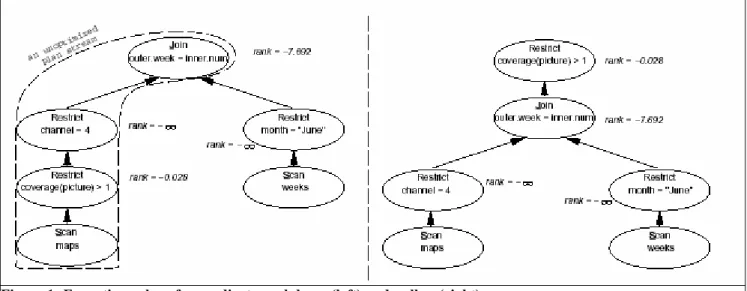
Also, it is crucial that the object relational optimizer put the expensive functions in the query plan at the correct places for the generation of scalable execution plans. This is motivated with the following Postquel (query language of POSTGRES) query from [3]
retrieve (maps.name) where
maps.week = weeks.number and weeks.month = “June” and maps.channel = 4 and coverage(maps.picture) > 1;
The query retrieves all channel 4 maps from week starting in June 17 showing more than 1% snow cover. Information about each week is kept in the weeks table requiring a join. In the example the function coverage is a complex image analysis function that may take thousands of instructions to compute. Now, a relational optimizer would try to restrict the maps and
weeks tables as much as possible before joining them (predicate pushdown). But in this case it is the wrong thing to do since coverage is an expensive function. Instead the optimizer should delay the restriction coverage(maps.picture) > 1
until after the join on maps and weeks to
minimize the number of instructions performed, so called predicate pullup. The two different execution plans for predicate pushdown and pullup are shown in Figure 1.
Figure 1: Executions plans for predicate pushdown (left) and pullup (right)
The execution time with predicate pushdown is 21 minutes. This is compared to the execution time with predicate pullup which is 3 sec. 3.4 Scans of inheritance hierarchies Suppose the new user-defined type student is added to our company database [1]. Consider the queries below extracting employees hired before a given date and with a given salary:
select name from only(emp)
where salary = 10000 and
startdate = < ’01/01/1990’; select name
from emp
where salary = 10000 and
startdate = < ’01/01/1990’;
Here the first query only extracts employees with the correct requirements while the second one extracts from the emp table and from the hierarchy under it i.e. the dept table. An approach for the optimizer to answer the second query could be to divide it into two sub-queries and then run them separately. A better way would be to try and union the two tables before applying the restrictions thus eliminating the overhead of processing two
queries. However, this is not such a good idea if one of the table have an index defined over some attribute and the other does not meaning that the index could not be utilized.
3.5 Joins over inheritance hierarchies In this section we assume that a user-defined type dept is also added to the employee database [1]. Concider the query below retrieving all employess and students working on the first floor:
select e.name from emp e, dept d
where e.dept = d.name and d.floor = 1;
The query could be replaced by the two sub-queries shown below:
select e.name
from only (emp) e, dept d where e.dept = d.name and d.floor = 1;
select e.name
from only (student_emp) e, dept d where e.dept = d.name and
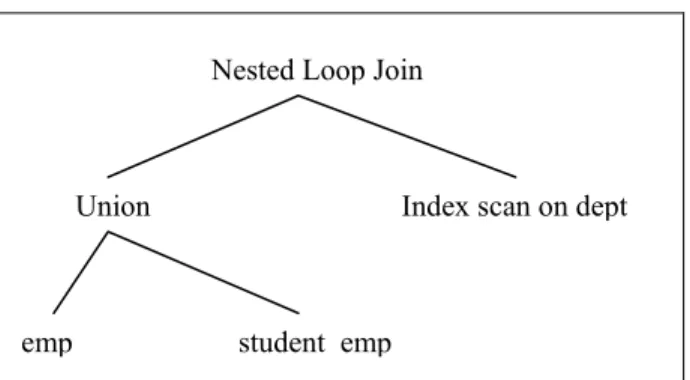
A possible action taken by the optimizer is to perform an index scan on the dept table and then join the result with the emp and
student_emp tables respectively. This is not a good strategy since the index scan on dept is done twice. A better execution plan, which should be generated by the optimizer, is the one shown in Figure 2.
Figure 2: Execution plan with one index scan of dept
Here the union of emp and student_emp is done before the join with dept meaning that the index scan on dept is only performed once.
4. Summary
In this paper the motivation behind, and characteristics of object-relational query processing has been discussed.
ORDBMS has evolved due to the need of users to model more complex real world problems in a way that is simple and intuitive for the developer.
Of course, this also put new demands on the optimizer to generate efficient execution plans. Instead of hard-coding all the information about fixed data types a table drive approach should be implemented allowing the creation of user-defined data types, functions, access methods and selectivity functions.
Particularly important is the development of a new more elaborate cost-model taking into account the impact of expensive functions and strategies for correct placing of these functions
in execution plans e.g. predicate pullup as shown in [3]
References
1. M.Stonebreaker, P.Brown:
Object-Relational DBMS – tracking the next great wave. Morgan Kaufman Publishers, 1999. 2. R.Elmasri, S.B.Navath: Fundamentals of
database systems. Pearson International Edition, 2007
3. J.Hellerstein, M.Stonebreaker: Predicate Migration: Optimizing Queries with Expensive Predicates. In Proc. ACM SIGMOD Conference on Management of Data, pp. 267—276, 1993.
Nested Loop Join
Index scan on dept
student emp emp