Pricing decisions in a two-echelon decentralized supply chain using bi-level programming approach

Winter 2015

Pricing decisions in a two-echelon decentralized supply chain using

bi-level programming approach

Maryam Mokhlesian1, Seyed Hessameddin Zegordi1*, Isa Nakhai Kamal Abadi1, Amir Albadvi1

1

Department of Industrial Engineering, Tarbiat Modares University, Tehran, Iran [email protected], [email protected], [email protected],

[email protected]

Abstract

Pricing is one of the major aspects of decision making in supply chain. In the previous works mostly a centralized environment is considered indicating the retailers cannot independently apply their decisions on the pricing strategy. Although in a two-echelon decentralized environment it may be possible that supply chain contributors have encountered with different market power situations which provide that some of them try to impose their interests in pricing and/or volume of the products. In such situations the leader-follower Stackelberg game or more specifically bi-level programming seems to be the best approach to overcome the problem. Furthermore, in this study we consider the impacts of disruption risk caused by foreign exchange uncertainty on pricing decisions in a multi-product two-echelon supply chain. Also it is assumed that the market is partitioned to domestic and international retailers with segmented market for each retailer. The purpose of this paper is to introduce decisions policy on the pricing such that the utility of both manufacturer and retailers is met. Since the proposed bi-level model is NP-hard, a simulated annealing method combining with Tabu search is proposed to solve the model. A numerical example is presented to investigate the effect of foreign exchange variation on the decision variables through different scenarios. The results from numerical example indicate that the international retailers are indifferent to the manufacture undergoes changes where the domestic retailers react to changes, dramatically.

Keywords: Bi-level programming, Decentralized supply chain, Pricing, Disruption risk, Simulated annealing and Tabu search

1*

Corresponding Author

1.

Introduction

In the real world, supply chains can procure their materials from domestic or off-shore suppliers. Explicitly, manufacturers can provide their needs from in-home manufacturing or by out-sourcing them. Furthermore, final products can be sold to the domestic or international retailers. Therefore, determination of price, amount of production or purchase as well as inventory and supplier or retailer selection is a sophisticated matter for each supply chain. Importing and/or exporting operations can encounter a supply chain to a variety of risks including foreign exchange risk, supply disruption risk, production disruption risk and other risks involving supply chains. Foreign exchange risk is one of the best known risks due to economy recession (Liu and Nagurney 2011).

In this study, we consider the pricing, importing and exporting decisions in a two-echelon supply chain consisting of one manufacturer and several retailers, segmented into two main classes: domestic and international. The supply chain confronts with uncertainty on the foreign exchange rate that leads to a high risk. Since each member of supply chain has a different power of decision making, the known single level programming models cannot sufficiently present this situation. To model this environment, bi-level programming is a promising approach such that the uncertainty is included by a scenario-based model.

2.

Literature review

In recent years, supply chains have paid more attention to the globalization. Blalock and Veloso (2007) investigated the role of importing on the productivity growth. Golini and Kalchschmidt (2011) aimed to suggest companies to improve their relationship with suppliers located in the different countries to face with uncertainty in the lead time and inventory level. Suzuki et al. (2011) hypothesized that vertical integration in the high-value export supply chains was only partial due to risks. Saygılı and Saygılı (2011) studied the structural changes as the integration into global production network to Turkish exports case. They found out that by exporting the non-traditional commodities, which have higher import and income sensitivity but lower real exchange rate elasticity, coefficients of the aggregate export function change accordingly. Liu and Papageorgiou (2013) considered cost, responsiveness and customer service level simultaneously for production, distribution and capacity planning of the global supply chains. Hammami and Frein (2014) developed a large scale optimization model to the problem of SC redesign while addressing decisions, costs, and complexity factors Also, They integrated transfer pricing in the model.

Because of variations in the environmental conditions, each supply chain may face with uncertainty risks. Tang (2006) reviewed different quantitative models to manage supply chain risks. The various supply chain risk management (SCRM) strategies studied in the research literature were linked to the actual practices. Tang and Tomlin (2008) presented five formalized models to demonstrate that firms could achieve significant strategic value by applying a risk reduction program which needed a relatively low level of flexibility. Trkman and McCormack (2009) presented a new approach to identify and predict the supply risk. This approach was based on the supplier’s attributes, performances and supply chain characteristics. Merschmann and Thonemann (2011) addressed the relationship between uncertainty, supply chain flexibility, and

firm performance. To achieve this aim, they used structural equation modeling. Klibi and Martel (2012) considered the assessment and the design of supply chain networks under uncertainty conditions by applying risk modeling approach. Hishamuddin et al. (2013) proposed a recovery model for a two-echelon serial supply chain with the transportation disruption. Cao et al. (2013) studied a coordination mechanism for a supply chain including one manufacturer and n Cournot competing retailers with consideration of the production cost and demands disruption. Huang et al. (2013) studied a pricing and production problem in a dual-channel supply chain with production cost disruption and investigated its effect on the original production plan. Qu et al. (2014) applied a non-scalarization method to a supply chain risk management problem with criteria considerations. Schmitt et al. (2015) investigated optimal channel design in a multi-location system with supply disruptions. They examined the expected costs and cost variances of the channel in both a centralized and a decentralized inventory system. Nooraie and Mellat Parast (2015) investigated the relation between supply chain visibility, supply chain risk and supply chain cost of new and seasonal products. They assumed that demand is probabilistic

One of the most important risks in the global supply chains is the foreign exchange rate risk. Gutierrez and Kouvelis (1995) developed a robust approach to international sourcing to consider uncertainty of the foreign exchange rate. This approach was relatively unaffected to the potential variations of the macroeconomic parameters over a planning horizon. Nagurney and Matsypura (2005) considered a three-stage global supply chain network to study the dynamics of its economy by taking into account the risk and uncertainty. They assumed that each members of supply chain may construct in the same or different country and may transact in different currencies. Goh et al. (2007) presented a stochastic model to the global supply chain network problem including several risks such as supply, demand and exchange risks as well as disruption. Liu and Nagurney (2011) considered supply chains with off-shore outsourcing activities to study the impact of foreign exchange risk and competition intensity. Arcelus et al. (2013) showed that in a newsvendor setting, if the retailer was not a risk-taker, the optimal policies are independent of the member endured the exchange risk. Hu and Motwani (2014) presented a methodology for minimizing downside risks related to the supplier base, supplier capacities, purchase-order-quantity, purchase-order-time, and selling-price.

This study makes several contributions to the field of purchasing, pricing and decentralized supply chain. First it provides an integrated model of risk and pricing in a bi-level system. Second, the process suggested in this paper will support companies to make decision about supplier selection, optimal pricing and global sourcing, independently. This study also provides a solution methodology to solve the bi-level programming model of decentralized supply chain.

The paper is organized as follows: First, in Section 2 is describing the model as a bi-level programming. Section 3 is devoted to the details of the proposed algorithm and parameter tuning as well as performance measurement. In Section 4, a numerical example is presented through. Finally, in conclusion we summarize the outputs of the study.

3.

Problem description

The unplanned and unanticipated occurrences which disrupt the routine flow of goods and materials within a supply chain are called “supply chain disruptions”. The supply chain

disruptions expose channel members to operational and financial risks. Generally, most supply chain disruptions can be classified into three categories, namely supply disruption, demand disruption, and miscellaneous risks. Supply disruption happens when suppliers cannot meet the orders from its customers. Demand disruption may be due to an unexpected decline or an unexpected grows in customer orders. Miscellaneous risks are risks that could potentially affect the costs of doing business, such as unexpected variation of purchasing costs, interest rates, currency exchange rates etc. (Li et al. 2010). In this paper, we focus on the miscellaneous risks due to foreign exchange risk.

Decentralization allows channel members to make decisions separately and independently that causes an improvement on each member’s utility. In such decentralized situations, the members may have different power to make a decision. This difference highlights the significance selection of the leader-follower Stackelberg game or the bi-level programming.

In this study, we consider a supply chain consisting of one manufacturer who produces several substitutable product and multiple retailers who buy one or more products from this manufacturer. Retailers are segmented to the domestic and international retailers. Raw materials are procured both internally and from off-shore suppliers. The manufacturer must decide on the amount of internal purchase and importing.

Since market power of supply chain members is different, applying single level programming approach is not helpful. Hence, bi-level programming model is used to decentralize the decisions. Bi-level programming model allows lower-level to decide independently to maximize its profit based on the decisions made by upper-level; however, in the single level model, decisions are made to maximize the profit of either only one member or whole channel. The manufacturer is considered as the leader (upper-level) and the retailers are considered as the followers (lower-level).

This structure is applicable to some situations like food industries with international brand in which the manufacturer produces several products and then, several retailers sell them.

3.1. Assumptions

Hereunder, we give the main assumptions used to develop the mathematical model.

 Products are substitutable.

 Suppliers are segmented to two classes of in-home and off-shore and retailers are considered as two parts of domestic and international.

 Each international retailer and off-shore supplier represents one country.

 Demand of each product follows a linear function of its price as well as the price of substitutable products.

 Shortage is not permitted.

 Manufacturer is Make-To-Order (MTO) i.e., it doesn’t hold any inventory and the production quantity is equal to the order size.

 Inventory of each product at retailer stage is considered.

 Manufacturer has finite supply capacity, i.e. has capacity constraint.

 Importing from several determined suppliers and exporting to numerous retailers are allowed.

 Importing and exporting have different tariffs and are calculated as a percentage of their values.

 There is a disruption in the rate of foreign exchange that leads to change in the values of import and export.

 Manufacturer shouldpay either tax of domestic sales or tariff of exporting incomes to the government.

 Procurement cost from both off-shore and in-home suppliers face uncertainty. 3.2. Notations

The following parameters are common for both manufacturer and retailer:

i Index of products. j Index of retailers.

k Index of suppliers.

N Number of products.

J Number of domestic retailers. J Number of international retailers. K Number of in-home suppliers. K _{Number of off-shore suppliers.}

The parameters and variables for the manufacturer (upper-level) are as follow:

i

P Annual production capacity for producti. i

C Production cost per unit of producti. k

F Procurement cost from the supplierk.

V The amount of required raw material. 1

 Tax rate for the manufacturer. 2j



Tariff rate of export incomes for the manufacturer to the international retailer j( 1, 2, ...,

jJ J JJ_).

3k



Toll tariff rate for the manufacturer from the off-shore supplier k(kK1,K2,...,KK ).

k

 Foreign exchange rate for the manufacturer with the off-shore supplier k(

1, 2,...,

kK K KK_).

j

 _{Foreign exchange rate for the manufacturer with the international retailer} j₍

1, 2,...,

jJ J JJ_).

k

y Decision variable, the amount of importing raw material from the off-shore supplier k(

1, 2,...,

kK K KK_).

x Decision variable, if the manufacturer pays tax, equals to 1 and otherwise, equals to 0. ij

w _{Decision variable, the wholesale price of product}i_{charged to the retailer} j_.

ij

a _{A constant in the demand function of the retailer} j _{for the product} i _{which represents} its market scale.

ij

b _{Coefficient of the}i_{th product’s demand elasticity for the retailer} j_. j

BD

Available budget of the retailer j. ij

D _{Demand of product}i_{from the retailer} j_. ij

O _{Ordering cost for the retailer} j_{per order of the product}i_. ij

h _{The retailer} j_{’s holding cost per unit of product}i_{‘s inventory per unit of time.}

1j

 _{Tax rate for the retailer} j_.

2j

 _{Toll tariff rate for the international retailer} j ₍jJ1,J2,...,JJ_). j

 _{Foreign exchange rate for the international retailer} j₍ 1 1, 2,..., ; 0 1, 2,..., .

j j J j j J J J J

         

). ij

z _{Decision variable, the amount of sales of product}i_{to the retailer} j_. ij

I _{Decision variable, the retailer} j_{’s inventory level of the product}i_. ij

p Decision variable, the retail price of producticharged by the retailer j. 3.3. Problem formulation

We consider single-manufacturer-multiple-retailer channel in which the manufacturer produces several substitutable products and the retailer sells only the manufacturer’s brand. Since demand of the retailers follows a linear function, they can be rewritten as follow:

( )

ij ij ij ij ij lj lj l i

D p a b p b p



  

_

, 1, 2,..., , 1,..., .

i i N

j j J J J J

  



    (1)

where the substitutability of the products is shown by

lj lj l i

b p 



.Also, it is assumed thatk_and j are stochastic because of uncertainty in the foreign exchange rate. Because of variability in the foreign exchange rate,Fk_{is stochastic, too. We suppose that these uncertain parameters follow a} trend around a predetermined value. Equations (2)-(4) indicate these trends:

0 1

(1 )

k k rk

   r1k U[ 1,1] (2)

0 2

(1 )

j j r j

   r_2j U[ 1,1] ₍₃₎

0 3

(1 )

k k k

F F r r3k U[ 1,1] (4)

where the random variablesr1k _, r2j_andr3k_{are the percentage of increasing or decreasing} indicating the variation rate and

0 k  , 0 j  and 0 k

F _{are the predetermined value. To confront with} the uncertainty, the several scenarios are considered which each scenario considers a fix value of variation rate.

The profit of the manufacturer is equal to the revenue achieved by the international and domestic sales subtracting by the costs. Its costs are the sum of procurement costs from suppliers, production cost as well as tax or tariff of exporting incomes to the government.

In the considered supply chain structure, each member has different market power such that manufacturer as the leader imposes the wholesale prices to the retailers. Based on these prices, retailers decide on the amount of purchase and the retail prices. Such situations can be modeled by bi-level programming models that its lower-level has multiple followers.

According to mentioned assumptions and notations, the proposed model can be constructed as follow to maximize the profit of each level:

1 1 1 1 1 1 1 1

3 1 2

1 1 1 1 1

max ( )

- (1 )

N J N J J K K K N J J

ij ij j ij ij k k i ij

i j i j J k k K i j

K K N J N J J

k k k k ij ij j j ij ij

k K i j i j J

w z w z F V y C z

F y x w z x w z

                                         



 





 





 



, 0, {0,1} ij k

w y  x

, 1, 2, , ; , 1, 2,...,

, 1, 2,. ;

.., .

k k K

i i N

K K j J K j J           

  (8)

, , _{1 1 1}

1 1

arg max ( )

ij ij ij

N N N

ij ij ij j ij ij ij ij ij

z p I _{i i i}

N j ij ij

i

z p w D O z h I

p z           









, 1, 2,...,

j j J J

   (9)

s.t.

( )

ij ij ij ij ij kj kj k i

D p a b p b p



  

_

ij ij ij

z I D i i, 1, 2,,N (11)

1

1 1 1 1

N N N N

ij j ij ij ij ij ij j ij ij j

i i i i

w  D O z h I  p z BD

   

   









, , 0

ij ij ij

z p I  i i, 1, 2,,N (13)

Objective function (6) maximizes the net profit of the manufacturer. Constraint set (7) ensures that production of product ishould not be greater than its capacity. Constraint set (8) shows the allowed sign of decision variables. Objective function (9) maximizes the net profit of each retailer to determine the order quantity for the manufacturer. Constraint set (10) shows the linear demand function of each product for the retailer. Constraint set (11) ensures that the demand of each product from each retailer should be met through its existing inventory and the order. Constraint (12) indicates the limited budget of each retailer. Constraint set (13) shows the allowed sign of decision variables.

4.

Proposed algorithm

Several researches in the literature are studied the approximation and metaheuristic algorithms to solve bi-level programming problem (BLPP). Weng and Huang (1996) developed an algorithm based on the tabu search (TS) to solve mixed-integer linear BLPP. Rajesh et al. (Rajesh et al. 2003) presented a tabu search based algorithm to solve the BLPP. Lan et al. (2007) combined neural network and tabu search algorithm to propose a method to solve BLPP. Wang et al. (2007) described an adaptive genetic algorithm for the linear bi-level programming problem to overcome the difficulty of determining the probabilities of crossover and mutation. Kuo and Huang (2009) developed a method based on particle swarm optimization (PSO) algorithm with swarm intelligence. Hu et al. (2010) proposed a novel neural network approach. Their proposed neural network was proved to be capable to generate optimal solution to the linear BLPP. Gao et al. (2011) developed a PSO based algorithm to solve pricing problems in a supply chain that was modeled as the BLPP. Wan et al. (2013) proposed a hybrid intelligent algorithm by combining the particle swarm optimization (PSO) with chaos searching technique to solve nonlinear BLPP.

Proposition 4.1: The proposed bi-level programming model of this study is a NP-hard problem.

Proof: See appendix A.

In this study, we hybridize tabu search and simulated annealing (SA) approach (SA_TS) to solve the proposed model.

SA is a simple form of local search algorithm (a descent algorithm) that starts with an initial solution which may be generated randomly. SA is based on the rules of statistical mechanics so that the annealing process involves warming and then slowly cooling a material to achieve a strong crystalline structure. The strength of this structure depends on the rate of cooling metals. Not enough high initial temperature or a fast cooling leads to defects. This condition cause that the cooling thing will not reach thermal equilibrium at each temperature. The SA algorithm simulates the energy variations in a system that is exposed to a cooling process until it converges to an equilibrium state. This mechanism can be adapted to an optimization problem. The objective function of the problem is similar to the energy state of the system. A solution of the optimization problem relates to a system state. The decision variables of the problem are like to the molecular positions. To escape from local optima and so to delay the convergence, at each iteration, a neighbor is generated, randomly. Moves that improve the objective function are always accepted. Otherwise, the neighbor is chosen with a specified probability that depends on the current temperature and the amount of Ewhich represents the difference in the objective value (energy) between the current solution and the generated neighboring solution (Talbi 2009).

An annealing schedule includes of an initial value of temperature, a cooling function, a number of neighbors to be searched at each temperature (to reach equilibrium state) and a stopping criterion to terminate the algorithm (Koulamas et al. 1994).

In the proposed algorithm, we consider the exponential cooling as a cooling function and the termination condition is achieved when we reach to the final temperature.

Tabu search (TS) viewed as a dynamic transformation of the neighborhood is combined by SA. Tabu search algorithm was proposed by Glover (1986). TS may be viewed as a neighborhood search. It admits non-improving solutions to escape from local optima when all neighbors are non-improving solutions. This procedure may leads to cycles; that is, previous visited solutions could be selected again.

To prevent cycles, TS removes the neighbors that have been previously visited. It remembers the recent search track. TS handles a memory of the solutions or moves recently used, which is called the tabu list. This tabu list is considered as the short-term memory. At each iteration, the short-term memory is updated. Since storing all visited solutions is time and space consuming, it should be checked, at each iteration, if a generated solution does not be in the list of all visited solutions. The tabu list usually has a constant size to store the tabu moves. Usually, the attributes of the moves are stored in the tabu list.

The tabu list may be too preventive; a non-generated solution may be forbidden. Yet for some conditions, called aspiration criteria, tabu solutions may be accepted. The acceptable neighbor solutions are those that are non-tabu or hold the aspiration criteria. In addition to the design of the neighborhood and initial solution generation, simple TS has the following issues (Talbi 2009):

Tabu list: The goal of using the short-term memory is to prevent revisiting the search from previously visited solutions. The size of tabu list is limited.

Aspiration criterion: A commonly used aspiration criteria involves of selecting a tabu move if it leads to a solution that is better than the best found solution. Another aspiration criterion may be a tabu move that generates a better solution among the set of solutions possessing a given attribute.

The tabu list of the proposed algorithm is the visited points and the tabu solution that is better than the best found solution is considered as the aspiration criterion.

Table 1 shows the notations of the algorithm parameters.

Table 1. The notations of the algorithm parameters

Parameters Notation

Tabu list size TL

Starting temperature T_max

Final temperature Tmin

Number of iteration at each temperature f

Number of neighbors ns

Number of temperature levels betweenT_maxand T_min q The procedure of the proposed SA_TS is as follow:

1. The initial solution of the leader and the follower are generated, randomly. 2. Cooling is commenced from the starting temperature.

3. The tabu list which is consisting of the visited solutions is initialized.

5. At each iteration, a neighbor is created by Shift mutation method. The Shift mutation method is the movement of a randomly chosen element to a random place.

6. Comparison of the current solution with the neighbor is done to find the trial solution.

7. If the next found solution is non-tabu and has a better objective function value, it is selected as the next solution.

8. The tabu list and aspiration criterion is updated.

9. Equilibrium condition is characterized as a given number of iteration executed at each temperature.

10. The best solution of the leader is determined based on the achieved followers’ solution. 11. Temperature is updated by use of exponential cooling calculated as follow:

max min

max

( )( 1)

( ) ; ; . 1, 2,..., .

1 l

T T q

T T l q

l q



     

     



(14)

12. These stages are repeated until the termination criterion is met; i.e. the temperature is greater than or equal to theTmin_.

The Fig. 1 shows the details of the proposed algorithm.

Template of the proposed SA_TS algorithm Input: cooling schedule

SL=SL0; %Generation of the leader’s initial solution SF=SF0; %Generation of the followers’ initial solution

based on the SL0 T=Tmax;%Starting temperature

Initialize the tabu list; %Visited solutions Repeat

Repeat %At a fixed temperature for a given number (ns) Generate a neighbor (SF′) for SF; %Shift mutation method

ΔE=f(SF′)-f(SF); %The change in the fitness

If ΔE≤0, Then SF= SF′; %Accept the neighbor solution

Else accept the SF′ with a probability E T e

 

;

Find the best admissible neighbor SF′; %Non-tabu or aspiration criterion holds SF= SF′;

Update tabu list & aspiration criterion; %Aspiration criterion: tabu solution that is better than the best found solution

Until Equilibrium condition %A given number of iteration (f) executed at each temperature T

Update the leader solution (SL) based on the best found followers solution (SF);

T=g(T); %Temperature update: exponential cooling Until Stopping criteria satisfied %T T_min

Output: Best solution found.

4.1. Parameter tuning

The run time and quality of the solutions are affected by the values of the algorithm parameters. Therefore, the parameters must be tuned carefully. For example, very high starting temperature causes a random local search. Furthermore, very low initial temperature leads a first improving local search algorithm. Moreover, the size of the tabu list is a critical parameter of TS that effect on the performance of the TS algorithm. The smaller value of the tabu list increases the probability of cycling. Larger values of the tabu list will provide many restrictions which forbid many moves (Talbi 2009).

One of the most popular methods to evaluate the importance of the parameters is ANOVA. Initial implementation of the test problems shows that, and have more effect on the both run time and quality of solutions than the other parameters. Therefore, the values of other parameters set as follow:

min

25; 10; 15; 20.

ns f  TL T 

In order to study the effect of the other parameters, we suggest a general factorial design of experiment (DOE). Two factors are considered in the experimentation and each factor is given two levels. The values of these levels are identified in Table 2. These levels are selected by experimentations.

Table 2. Levels of DOE

Parameters Label Levels

max

T A1 40 70

q A2 20 25

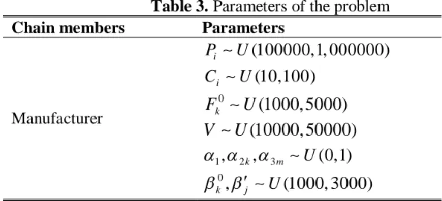
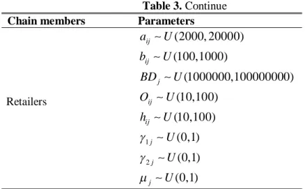
For each combination of the four factors under study, 45 randomly generated problems are solved and the responses are measured. These problems are selected from a given data set shown in Table 3.

Table 3. Parameters of the problem

Chain members Parameters

Manufacturer

(100000,1, 000000)

i P U

(10,100)

i C U

0

(1000, 5000)

k F U

(10000, 50000)

V U

1, 2k, 3m U(0,1)

   

0

, (1000, 3000)

k j U

Table 3. Continue

Chain members Parameters

Retailers

(2000, 20000)

ij a U

(100,1000)

ij b U

(1000000,100000000)

j BD U

(10,100)

ij O U

(10,100)

ij h U

1j U(0,1)

 

2j U(0,1)

 

(0,1)

j U

 

Table 4 shows the analysis of variance (ANOVA) while the response is the sum of fitness function values.

Table 4. 22 factorial design

Sources df SS MS F P-value

A1 1 1.21E+24 1.21E+24 5.94E-03 0.94

A2 1 1.19E+24 1.19E+24 5.82E-03 0.94

A1×A2 1 1.20E+24 1.20E+24 1.98E+03 <0.001

Error 176 3.58722E+28 2.03819E+26

Total 179 3.59E+28

According to the Table 4, the interaction between parameters is significant. Student-Newman-Keules test (Hicks 1993) is used to tune the significant parameters. The results of parameter tuning are as follow:

max 40, 25.

T  q

4.2. Performance measurement

In order to evaluate the proposed algorithm (SA_TS), the performance is compared with that of an existing PSO algorithm in the literature proposed by Gao et al. in 2011.The best solution obtained for each instance generated in section 4.1 by each of the two algorithms (PSO or SA_TS) is named Bestsol and the solution obtained for each instance by SA_TS (the proposed algorithm) is named Algsol. So, relative percentage deviation (RPD) as a comparison criterion is calculated as follows:

lg

100

sol sol

sol

Best A

Best

Table 5 shows the results of comparison.

Table 5. Results of comparison

Problem size ( , ,N J J K K, , ) _{Average of RPD} Average of SA_TS run time (second)

Small (10,25,5,10,5) 0.0% 120

Medium (25,50,10,20,10) 3.25% 615

Large (50,100,20,30,20) 6.46% 1110

According to Table 5, the greater problem size will lead to the larger deviation due to larger feasible space which should be searched. It is inferred from these values that the proposed algorithm is 3.25% below the best obtained solution on average in the medium size and 6.46% in the larger size.

5.

Computational results

To evaluate the effect of foreign exchange rate variations on the decisions, the considered scenarios are the extreme cases. For this sake, a small problem with 10 products, 25 domestic retailers, 5 international retailers, 10 in-home suppliers and 5 off-shore suppliers is assumed that its parameters are generated randomly by distribution mention in Table 3. The results of comparisons are demonstrated in Table 6. The average of each decision variable for each product is indicated to simplify the understanding.

It can be derive from the results that increasing in the foreign exchange rate leads to changes in the decisions and profit of the manufacturer and the domestic retailers, while it has no effect on the decisions and profit of the international retailers. These results are inferred as follow:

The wholesale price charged by the manufacturer to the international retailers does not change because the variation in the foreign exchange rate is related to the manufacture’s country not to them. Therefore, the amount of their purchase will not change, too.

The manufacture amends increasing in its procurement costs through increasing in the wholesale price charged to the domestic retailers. It leads to decrease in their amount of purchase. The other way to amend these costs gains through exporting incomes that are grew due to increasing foreign exchange rate. Hence, increment in the foreign exchange rate increases the manufacture’s profit.

As the wholesale prices for the domestic retailers are raised by growth of the foreign exchange rate, the retail prices must increase, too. Therefore, the profit of the domestic retailers is decreased by increasing in the foreign exchange rate.

Table 6. Comparison results

6.

Conclusion

In this study, a supply chain was considered which consists of one manufacturer who produces several substitutable products and multiple retailers who buy one or more products from this manufacturer. Retailers were segmented into the domestic and international retailers. Raw materials were procured both internally and from off-shore suppliers. The manufacturer intends to decide on the amount of internal purchase, external purchase, pricing and exporting.

V

ar

iat

ion

s

Average of decision variables Average of profit

Followers Leader

yk

international domestic

108 128 419 2,933 57,285 62,529

624,300 428,163,543,736 2,059,492,511,796 13,214,000,000

104 _{118 196 861 51,57 69,633} 111 118 162 1,464 39,69 62,532 102 _{125 162 611 58,46 45,271} 113 136 444 3,524 49,48 49,094

99 122 147 249 41,80 40,220 102 116 113 928 52,59 52,918 107 137 436 4,357 58,70 43,127 107 124 129 1,174 39,22 34,888 93 103 194 118 47,44 47,535 109 128 421 2,933 57,28 62,529

4,791,400 428,163,543,736 2,043,624,789,543 689,540,000,000

104 118 199 861 51,57 69,633 112 118 162 1,464 39,70 62,532 102 125 163 611 58,47 45,271 115 136 445 3,524 49,47 49,094 101 122 157 249 41,78 40,220 100 116 114 928 52,61 52,918 107 137 436 4,357 58,70 43,127 106 124 129 1,174 39,22 34,888 93 103 196 118 47,44 47,535 109 128 421 2,933 57,29 62,529

4,342,100 428,163,543,736 2,040,045,961,524 1,249,400,000,000

104 118 199 861 51,57 69,633 112 118 163 1,464 39,70 62,532 103 125 164 611 58,46 45,271 112 136 445 3,524 49,49 49,094 101 122 157 249 41,79 40,220 102 116 116 928 52,59 52,918 108 137 436 4,357 58,69 43,127 106 124 130 1,174 39,22 34,888 93 103 197 118 47,44 47,535

To achieve this goal, first the problem was formulated as a bi-level programming problem. Then, since it is proven that the problem is NP-hard, a metaheuristic algorithm is proposed to solve the model based on the hybridization of simulated annealing and tabu search. The proposed algorithm was compared with an existing PSO method. The implementation of test problems demonstrated an acceptable preference of SA_TS to the PSO.

The results based on numerical example demonstrated that variation in the foreign exchange rate has no impact on the international retailers’ decisions and profit, while changed the decisions and profit of the domestic retailers. Increasing in the foreign exchange rate raised the profit of the manufacturer through increment in the wholesale prices charged to the domestic retailers and exporting incomes.

Our analysis might also have some limitations. Firstly, we assume one-manufacturer-multiple-non-competitive retailers. More research can be extended to multiple competing retailers and manufacturers. Secondly, the disruption caused by foreign exchange risk is considered in this study. It can be extended to the other risks that could potentially affect the costs of doing business, such as unexpected changes to purchasing costs, interest rates and currency exchange rates.

References

Arcelus, F. J., Gor, R., & Srinivasan, G. (2013). Foreign exchange transaction exposure in a newsvendor setting. European Journal of Operational Research, 227(3), 552-557.

Blalock, G., &Veloso, F. M. (2007). Imports, productivity growth, and supply chain learning. World Development, 35(7), 1134–1151.

Cao, E., Wan, C., & Lai, M. (2013). Coordination of a supply chain with one manufacturer and multiple competing retailers under simultaneous demand and cost disruptions. International Journal of Production Economics, 141, 425–433.

Gao, Y., Zhang, G., Lu, J., & Wee, H. M. (2011). Particle swarm optimization for bi-level pricing problems in supply chains. Journal of Global Optimization, 51, 245-254.

Glover, F. (1986). Future paths for integer programming and links to artificial intelligence. Computers & Operations Research, 13, 533-549.

Goh, M., Lim, J. Y. S., & Meng, F. (2007). A stochastic model for risk management in global supply chain networks. European Journal of Operational Research, 182, 164–173.

Golini, R.,& Kalchschmidt, M. (2011). Moderating the impact of global sourcing on inventories through supply chain management. International Journal of Production Economics, 133, 86–94.

Gutierrez, G. J.,& Kouvelis, P. (1995). A robustness approach to international sourcing. Annals of Operations Research, 59, 165-193.

Hammami, R., & Frein, Y. (2014). Redesign of global supply chains with integration of transfer pricing: Mathematical modeling and managerial insights. International Journal of Production Economics, 158, 267-277.

Hicks, C. R. (1993).Fundamental concepts in the design of experiments, Fourth ed., New York: Oxford University Press.

Hishamuddin, H., Sarker, R. A. & Essam, D. (2013). A recovery model for a two-echelon serial supply chain with consideration of transportation disruption. Computers & Industrial Engineering, 64, 552–561. Hu, T., Guo, X., Fu, X., & Lv, Y. (2010). A neural network approach for solving linear bilevel programming problem. Knowledge-Based Systems, 23, 239–242.

Hu, X., &Motwani, J. G. (2014). Minimizing downside risks for global sourcing under price-sensitive stochastic demand, exchange rate uncertainties, and supplier capacity constraints. International Journal of Production Economics, 147, 398-409.

Huang, S., Yang, C., & Liu, H. (2013). Pricing and production decisions in a dual-channel supply chain when production costs are disrupted. Economic Modelling, 30, 521–538.

Lan, K. M., Wen, U. P., Shih, H. S., & Lee, E. S. (2007). A hybrid neural network approach to bilevel programming problems. Applied Mathematics Letters, 20, 880–884.

Li, J., Wang, S., & Cheng, T. C. E. (2010) Competition and cooperation in a single-retailer two-supplier supply chain with supply disruption. Int. J. Production Economics, 124, 137–150.

Liu, S.,& Papageorgiou, L. G. (2013). Multiobjective optimisation of production, distribution and capacity planning of global supply chains in the process industry. Omega, 41, 369–382.

Liu, Z., &Nagurney, A. (2011). Supply chain outsourcing under exchange rate risk and competition. Omega, 39, 539–549.

Klibi, W., &Martel, A. (2012). Scenario-based Supply Chain Network risk modeling. European Journal of Operational Research, 223, 644–658.

Koulamas, C., Antony, S. R., & Jaen, R. (1994). A survey of simulated annealing applications to operations research problems. Omega, 22(1), 41-56.

Kuo, R. J.,& Huang, C. C. (2009). Application of particle swarm optimization algorithm for solving bi-level linear programming problem. Computers and Mathematics with Applications, 58, 678-685.

Merschmann, U.,& Thonemann, U. W. (2011). Supply chain flexibility, uncertainty and firm performance: An empirical analysis of German manufacturing firms. International Journal of Production Economics, 130, 43–53.

Nagurney, A., &Matsypura, D. (2005). Global supply chain network dynamics with multicriteria decision-making under risk and uncertainty. Transportation Research Part E, 41, 585–612.

Nooraie, S. V., & Mellat Parast, M. (2015). A multi-objective approach to supply chain risk management: Integrating visibility with supply and demand risk. International Journal of Production Economics, 161, 192-200.

Qu, S. J., Goh, M., De Souza, R., & Wang, T. N. (2014). Proximal Point Algorithms for Convex Multi-criteria Optimization with Applications to Supply Chain Risk Management. Journal of Optimization Theory and Applications, 163(3), 949-956.

Rajesh, J., Gupta, K., Kusumakar, H. S., Jayarama, V. K., & Kulkarni, B. D. (2003). A tabu search based approach for solving a class of bilevel programming problems in chemical engineering. Journal of Heuristics, 9, 307–319.

Sahni, S. (1974). Computationally related problems. SIAM Journal on Computing, 3, 262–279.

Saygılı, H.,& Saygılı, M.(2011).Structural changes in exports of an emerging economy: Case of Turkey.

Structural Change and Economic Dynamics, 22, 342– 360.

Schmitt, A. J., Sun, S A., Snyder, L. V., & Shen, Z. M. (2015). Centralization versus decentralization: Risk pooling, risk diversification, and supply chain disruptions.Omega, 52, 201-212.

Suzuki, A., Jarvis, L. S.,&Sexton, R. J. (2011). Partial vertical integration, risk shifting, and product rejection in the high-value export supply chain: the Ghana pineapple sector. World Development, 39(9), 1611–1623.

Talbi, E. (2009).Metaheuristics: from design to implementation, New Jersey:John Wiley & Sons, Inc., Hoboken.

Tang, C. S. (2006). Perspectives in supply chain risk management. Int. J. Production Economics, 103, 451–488.

Tang, C.,& Tomlin, B. (2008). The power of flexibility for mitigating supply chain risks. International Journal of Production Economics, 116, 12–27.

Trkman, P.,& McCormack, K.(2009).Supply chain risk in turbulent environments—A conceptual model for managing supply chain network risk. Int. J. Production Economics, 119, 247–258.

Wang, G., Wang, X., Wan, Z., & Jia, S. (2007). An adaptive genetic algorithm for solving bilevel linear programming problem. Applied Mathematics and Mechanics (English Edition), 28(12), 1605–1612. Wan, Z., Wang, G., & Sun, B. (2013). A hybrid intelligent algorithm by combining particle swarm optimization with chaos searching technique for solving nonlinear bilevel programming problems. Swarm and Evolutionary Computation, 8, 26–32.

Weng, U. P., &Huang, A. D. (1996). A simple Tabu Search method to solve the mixed-integer linear bilevel programming problem. European Journal of Operational Research, 88, 563-571.

Appendix A:

To prove a problem is NP-hard, a known NP-hard problem should be reduced to this problem through a polynomial-time transformation between problems. Hence, to show the complexity of the proposed problem, consider the below non-convex quadratic programming (QP) model:

1

min ( ) max ( )

2

T T

F X XQX dX F X

     (A.1)

AX b (A.2)

Suppose that X ( ,x x x x x_{1 2}, ₃, ₄, ₅), d(0, 0, , , (1C C F ₃), 0 0 0 0 0

1 1 1 1 1

A_{ } _

    

 

and

0 P b_{  } 

 

. Qis as follows:

1

0 0 1 0 0 0 0 0

x Q     2 1 2

- (1 (1 ) ) 0 1 0 0 0 0 0 - (1 (1 ) )

x x x          

   0 0 0 0 0 0 0 0

               

where x{0,1}. According to the above definitions, the mentioned QP can be rewritten as follow:

1 3 2 4 5 3 4 3 5 2 2 4 1 1 3

max ( )F X x x x x F V( x )C x( x ) F x (1x) x x x x x (A.3) s.t.

3 4

x x P (A.4)

1, 2, 3, 4, 5 0

x x x x x  (A.5)

Qis calculated as follows: Ifx0:

2

2

0 0 1 0 0

0 0 0 (1 ) 0

1 0 0 0 0

0 (1 ) 0 0 0

0 0 0 0 0

Q         _{  }                  

Ifx1:

1

1

0 0 (1 ) 0 0

0 0 0 0

(1 ) 0 0 0 0

0 0 0 0

0 0 0 0 0

Q          _{ }                  

Since theQin the each of two cases is not PSD ( 0, 0₂ 1), it is interpreted that the above nonconvex quadratic programming problem is NP-Hard (Sahni 1974).

Consider the below transformation for the parameters and decision variables of the above QP:

1 ij

x w i1, 2,..., ;N j1, 2,..., .J (A.6)

2 ij

x w i1, 2,..., ;N jJ1,J2,...,J J. (A.7)

3 ij

x z i1, 2,..., ;N j1, 2,..., .J (A.8)

4 ij

5 k

x y kK1,K2,...,KK. (A.10)

j

  jJ1,J 2,...,JJ. (A.11)

k

F F k1, 2,..., .K (A.12)

i

C C i1, 2,..., .N (A.13)

i

PP i1, 2,..., .N (A.14)

k

  kK1,K2,...,KK. (A.15)

3 3k

  kK1,K2,...,KK. (A.16)

2 2j

  jJ1,J 2,...,JJ. (A.17)

The mentioned QP is reduced to the manufacturer’s problem (p1) as a sub-problem of the proposed problem (main problem) through these transformations. Since this non-convex quadratic programming problem is NP-hard, the manufacturer’s problem is NP-hard, too.

As (p1) is NP-hard, the main problem is NP-hard, too, because the degree of the complexity of a sub-problem is not less than the main problem.