Vol. 5, No. 2, pp 63-79 Summer 2011
Coordinating a Seller-Buyer Supply Chain with a Proper Allocation of
Chain’s Surplus Profit Using a General Side-Payment Contract
Sina Masihabadi (1985-2011),Kourosh Eshghi1
1 Industrial Engineering Department, Sharif University of Technology, Zip code 14588-89694, Tehran, Iran [email protected]
ABSTRACT
In this paper, seller-buyer supply chain coordination with general side-payment contracts is introduced to gain the maximum possible chain profit. In our model, the logistics costs for both buyer and seller are considered and the final demand is also supposed to be a decreasing function of the retail price. Since parties aim to maximize their individual profits, the contractual parameters are set in a way that these decisions become aligned with system optimal decisions. Therefore, a side payment contract is suggested in our model to assign the chain surplus profit to the chain members such that they have no intention to leave the coalition. Then, we change the contract into a quantity discount-like contract which makes the contract much easier to be implemented in a real situation. The model will also be extended to include two buyers and a single seller. Finally, by numerical analysis, we show that by using this kind of contract, a significant improvement in the chain members’ profits and the total chain revenue will be achieved.
Keywords: Seller-Buyer Supply Chain, Supply Chain Coordination, Supply Chain Contracts, Game Theory.
1. INTRODUCTION
In the last two decades, both academicians as well as practitioners have shown more interest on the supply chain management. In fact, market globalization, increased competition and reduced gap between products in terms of quality and performance; have forced researchers to rethink about how to manage business operations more efficiently. A supply chain consists of a number of distinct entities who are responsible for converting the raw material into finished product and make them available to final customer to satisfy their demand in time at least possible cost (Sarmah et al., 2006).
The optimal performance of a supply chain needs a proper cooperation of a set of activities, but these activities are not always interesting for chain members, because they want to maximize their individual profits and this may contradict these activities and cause the poor performance of the total chain. One of the most important topics discussed in supply chain management is supply chain coordination to integrate the operations performed by distinct chain members and achieve the
Corresponding Author
maximum chain-wide profit. A contract is said to coordinate the supply chain if the set of supply chain optimal actions is Nash equilibrium, i.e., no firm has a profitable unilateral deviation from the set of supply chain optimal actions (Cachon, 2003). In a coordinated supply chain, a decentralized channel (a channel in which each member acts as an independent decision maker), should perform in a centralized pattern, i.e. where all decisions are made by one member. Leng and Parlar (2010) introduced appropriate buy-back and lost-sales cost-sharing contracts to coordinate decentralized assembly supply chain so that when all the suppliers and the manufacturer adopt their equilibrium solutions, the system-wide expected profit is maximized.
Among the most common ways used for supply chain coordination are side-payment contracts. Robin and Carter (1995) defined side-payment as ‘‘an additional monetary transfer between supplier (seller) and buyer that is used as an incentive for deviating from the individual optimal policy”.
The number of publications related to supply chain coordination with side-payment contracts has rapidly increased during the last decade (Leng and Zhu, 2009). In most of them, the proper allocation of profit surplus has been completely neglected and they have assumed an arbitrary allocation of surplus profit; but in practice, this can lead to terminating the formed coalition between chain members. In contrast, some papers have just discussed the allocation of profit surplus assuming that all supply chain members voluntarily cooperate for supply chain coordination. There are some good literature reviews on the seller-buyer coordination, among them we can name: Nagarajan and Sosic (2008), Lai et al. (2009), Arshinder et al. (2008) and Sarmah et al. (2006).
Hezarkhaniand Kubiak (2010) provided a systematic overview of coordinating contracts in supply
chain through highlighting the main concepts, assumptions, methods, and presented the state-of-the art research in this field. Breiter et al. (2009) presented a review article in this field and explicitly addressed new trends in supply chain management, namely, the consideration of multi-tier value-added processes, the coordination of multi-sourcing/customer relationships and the handling of complex bill-of-materials structures.
To the best of our knowledge, Leng and Zhu (2009) is the only case, in which there is a particular discussion on how a proper side-payment contract can be obtained to ensure that the chain-wide performance is improved and all supply chain members are also better off than in the non-cooperative case. However, the model presented in Leng and Zhu (2009) assumes a news vendor setting and has been developed without considering the logistics costs of the vendor. In addition, they perform no numerical analysis on the proposed contract to measure the amount of improvement achieved by using the contract. Furthermore, they provided a procedure and applied it to four special games. In this paper we extend their model by considering the logistics costs and perform an extended numerical analysis on the relations obtained in the model.
In our model, a supply chain coordination along with the proper allocation of profit surplus to the chain members is considered. Furthermore, it is assumed that there is an inventory holding cost for both seller and buyer and the final demand is a decreasing function of the retail price. Although the demand behavior in our model is not considered to be stochastic, its dependency to the price caused the changes to retail price to affect market demand. One of the important characteristics of our model is to apply the equilibrium concept by fair allocation of profit surplus which can ensure the stability of coalition between the chain members. The numerical analysis of the model shows a significant improvement on the chain-wide Income.
The remaining sections are organized as follows: section 2 is an introduction section in which some important concepts for developing the contract are discussed. Section 3 is devoted to presenting the model and developing the proper general side-payment contract for it. In section 4, we change the contract into an easy to implement, quantity discount-like contract. In section 5, the extension of the model, to a model containing two buyers buying from a single seller is discussed. Section 6 reports the results obtained from numerical analysis. Finally, the conclusion of the paper and suggestions for further research are summarized in section 7.
2. PRELIMINARIES
In this section, some important concepts from the literature related to supply chain management and game theory are discussed. As mentioned before, in our model, there is a single buyer who buys from a single seller and we can consider the seller as player one and the buyer as player two, who
make decisions and to maximize their income functions denoted by ( , ) and ( , ),
respectively. A Nash equilibrium ( , ) must satisfy the following condition (Leng and Zhu,
2009)
( , ) ≥ ( , ) ∀
( , ) ≥ ( , ) ∀
If there is not any coordination mechanism (e.g. a side-payment contract) used in the chain, it is called the non-cooperative case. The goal of our model is to develop a proper side-payment contract, under which the players have their equilibrium solutions identical to the globally-optimal solutions. This will maximize the overall (system-wide) payoff. Furthermore, the players should act better under this contract than in the non-cooperative game without side-payments. To achieve this aim, we add two terms to income functions to form the income functions under the side-payment contract
( , ) = ( , ) − ( , ) − ( , ) = ( , ) + ( , ) +
where ( , ) is the amount paid by player1 to player 2 and depends on the decisions made by the
two parties and is the constant payment term from player1 to player 2 to ensure that both players will gain more revenue in comparison with the non-cooperative case. The value of should obtain
by the negotiation between these two players. By adding the term ( , ) to the income functions,
the chain will be coordinated somehow that the Nash equilibrium of each party, denoted by( , ),
be the same as the optimal solution maximizing the chain-wide profit. Before taking into consideration, two players have incomes as follows
( ∗, ∗) = ( ∗, ∗) − ( ∗, ∗) ( ∗, ∗) = ( ∗, ∗) + ( ∗, ∗)
The surplus or deficit for each player, with respect to the non-cooperative case, is obtained as
= ( ∗, ∗) − ( , ) = 1,2 .
If ≥ 0 then player gains a surplus of , else he/she has a deficit of | | and probably in this
( , ) is the chain-wide income when player makes decision . is the surplus of the whole chain and in order to ensure the stability of the coalition, it must be properly allocated to both parties.
To achieve a fair unique way for allocating the surplus, we turn our attention to cooperative game theory. In two players nonzero-sum games, there are two main concepts for surplus allocation: Nash arbitration (bargaining) scheme and Shapely value. We refer to Nagarajan and Sosic (2008), for a good discussion about these concepts and also the axioms used in the Nash theorem.
Using the above assumptions, Leng and Zhu (2009) have proposed two corollaries about the allocation of profit surplus in a seller-buyer supply chain, which we use in developing our side-payment contract. The proofs are easy and straightforward ( Leng and Zhu, 2009).
Corollary 1. Nash arbitration scheme suggests that the system-wide surplus is equally allocated between two players as follows
= = ( ∗, ∗) , = /2.
where = [ ( ∗, ∗) − ( , )] = 1, 2.
Corollary 2. If the overall surplus is equally allocated as suggested by Nash arbitration scheme, then the constant side-payment term is determined as follows
=∑ (−1) [ ( ∗, ∗) + (−1) ( ∗, ∗) − ( , )]
2
3. MODEL STRUCTURE
In this section, we study a supply chain that includes a single seller and a single buyer. The seller produces or buys a product and wholesales it to the buyer in batches. The buyer retails that product to the final customer. The logistics costs are considered for both parties in our model. The buyer income function is based on the model introduced by Abad (1988) and we use the general assumptions and the seller income function as Esmaeili (2009) with the important difference that, here, the order quantity is a decision that should be made by the buyer not the seller. This assumption is more common and practical in real world, because usually it is the buyer who decides how much to order.
3.1. Notations
Decision variables
lot size in units determined by the buyer
retail price which is a decision of the buyer ($/unit)
Parameters
scaling constant for demand function ( > 0)
ℎ inventory holding cost per unit per year for the seller
ℎ inventory holding cost per unit per year for the buyer (ℎ ≥ ℎ )
price elasticity of demand function (1 < < 2) (This parameter is a measure of price
influence on demand and appears as the power of price in the demand function.)
wholesale price per unit, charged by the seller (ν > + / )
buyer’s ordering cost ($/order) seller’s set up cost ($/set up)
seller’s production cost including purchasing cost ($/unit) seller’s production rate (units/day)
annual demand as a function of p
market demand rate (units/day)
3.2. Assumptions
All parameters are deterministic and known in advance.
Planning horizon is infinite.
Shortages are not allowed, hence, the production rate is greater than or equal to the
demand rate and, without loss of generality, we will assume them to be linearly related by
the equation = , ≥ 1.
The seller’s set up cost is greater than the buyer’s ordering cost ( > ).
Demand is assumed to be a function of retail price and is modeled as ( ) = (Lee
et al., 1996).
3.3. Developing the contract
The buyer’s income is modeled as follows (Abad, 1988)
( , ) = − − − 0.5ℎ = − − − 0.5ℎ (1)
Moreover, the seller’s income is defined as follows (Esmaeili, 2009)
( , ) = − − − 0.5ℎ
= − − − 0.5ℎ (1 − ) (2)
Now a side-payment contract is developed with some special properties for the supply chain as
discussed before. First, we calculate the buyer’s Nash equilibrium point ( , ). It can be shown
that ( , ) is a strictly pseudo concave function (Esmaeili, 2009) with respect to for a fixed .
Hence, the first-order condition of ( , ) with respect to determines the unique that
= ( ) (3) Now, substitution of (3) into (1) and simplification implies that
( ( ), ) = − 0.5ℎ (4)
This function is concave in (refer to Appendix A (2)), Therefore, optimal value of will be found after some algebraic operations (Appendix A (1)) as
=
. (5)
That is clear from (3) and (5), that each and value is related to each other. Thus, in order to perform the numerical analysis, it is necessary to derive an independent equation for one of them. This equation is obtained at Appendix A (3).
Note that, by setting the first derivative of (2) with respect to , equal to zero, we obtain =
. , which is the same as (5). Hence, we conclude that the buyer equilibrium solution must
satisfy the following conditions
= − 0.5ℎ = 0 (6)
= (− + 1) + + = 0 (7)
To determine the proper transfer payments between two players, we should study the effects of one’s decisions on both parties’ incomes. First, we study the effect of the order quantity
= − 0.5ℎ (8)
By solving (8), we obtain =
. (9)
Since we have = −2 < 0 , then maximizes the seller’s income. Note that is a
decision to be made by the buyer and in the non-cooperative case it is obtained from equation(5).
According to the assumptions, > , ≥ 1 and ℎ ≥ ℎ , hence, > will be held. Thus, the
seller wants the buyer to increase his/her order size from to by paying him/her a transfer
payment as compensation. We model this amount as follows
( ) = ( − ) . (10)
It is clear that seller should be willing to pay until reaches the seller’s optimal lot size amount ( ),
( )should not be positive for these s. This must be reflected in the equation we will derive for , later in this section. On the other hand, we have
= + − (11)
If the seller has a positive profit margin ( > + ), then < 0. This shows that the seller’s
income decreases with an increase in retail price. This behavior was completely expectable since
increasing retail price would reduce demand and cause the seller’s less profit. Only when < +
, the seller suffers a loss by selling each unit and since no shortage is permitted, he/she wants the demand to be reduced, thus the retail price to be increased. In this case the seller is willing to pay the buyer to reduce his/her price. We model this payment as follows
( ) = ( − ) (12)
Where > 0 must be held, since the seller is always willing to reduce the retail price. Considering these side-payment terms, the income functions of both members are given by
( , ) = ( , ) − ( − ) − ( − ) − (13)
( , ) = ( , ) + ( − ) + ( − ) + (14)
Note that, after considering the side-payment terms, the chain must be coordinated. Subscript “ ” is used for the variables corresponding to the coordinated chain. Now, the values of contractual parameters must be found when the chain becomes coordinated.
Considering the results obtained by the buyer’s equilibrium solution and equations (13) and(14),
the Nash equilibrium in cooperative case must satisfy the following equations (the subscript “ ”
indicates the Nash equilibrium in the coordinated chain)
( , )
= − 0.5ℎ + = 0 (15)
( , )
= (− + + ) + − = 0 (16)
Now, we consider chain-wide income function. This function equals the sum of two members’ incomes, which yields
( , ) = − − − 0.5 (ℎ + ℎ ) (17)
To obtain the optimal solution for the system, ( ∗, ∗), we use the similar approach as finding the
buyer’s Nash equilibrium. The form of the function with respect to , is the same as (3), thus ( , ) is strictly pseudo concave in (Esmaeili , 2009) ; hence, we can obtain a unique which
maximizes the function for a fixed . This is shown in equation(18) (For simplicity, we set
+ = ).
Substituting (18) into (17) implies that
( ∗( ), ) = − 0.5 (ℎ + ℎ ) (19)
This function is concave in (Appendix A (5)), thus, the optimal will obtain after some algebraic operations (Appendix A (4)) as follows
∗= ∗
. ( ) (20)
As the previous case, an independent equation is derived for ∗ (Appendix A (6)).
But, equation (20), is the same as the solution to the first order derivative of ( , ) w.r.t. . Therefore, ∗and ∗ must satisfy the following conditions
( , )
= ∗ − ∗+ + ∗ + ∗ = 0 (21)
( , )
= ∗ ∗ − 0.5(ℎ + ℎ ) = 0 (22)
Comparing (21) and (22) to (16) and (15) respectively, will allow us to compute and . By
coordinating the chain, there would be no difference between with ∗ and with ∗ and we
obtain
= ∗ ∗ − 0.5ℎ (23)
Note that, substituting obtained from equation (9) into (23), will imply = 0. This is reasonable, because if the lot size to be ordered by the buyer is the same as the one maximizing the seller’s profit, he/she will have no intention to change this amount. In fact, from equation (23), it is clear
that for ≤ ∗≤ , we have ≥ 0 and the seller is ready to pay for increasing in this range.
However, for the amounts more than the optimal lot size for the seller ( ), the computed would be negative. For , we obtain
= ∗ (ν − − ) (24)
Previous discussion about the inequality > + , implies that > 0, as it was expected.
Finally, using corollary 2, we obtain the following equation for the constant term
= [ ( , , ) − ( , , )] − [ ( , , ) − ( , , )] (25)
Now, all contractual parameters are found, therefore the side-payment contract is developed.
4. A PRACTICAL QUANTITY DISCOUNT-LIKE CONTRACT
A proper contract, in addition to coordinating the chain and proper profit allocation, should be easy to implement and applicable in practice. Among classic side-payment contracts, quantity discount contract is less complicated in the form. In fact, under this contract, one just needs to relate the
order quantity with unit price and the payment from the buyer to the seller would be easy to determine (for a full discussion about this kind of contract, please see Sarmah et al., 2006). If we change our general side-payment contract, which is complicated as a contract and can cause ambiguities and problems in practice, to a contract similar to quantity discount, we will take an important step for its successful implementation.
In this section, a quantity discount-like contract, which coordinates the chain and allocates the profit surplus between the members similar to the previous general side-payment contract, will be studied.
Corresponding to equation(1), we form the buyer’s income function under the quantity discount
contract as
( , ) = − ( ) − − 0.5ℎ (26)
where ν( ) is a function of and shows the wholesale price of each unit when the buyer orders
units. Now, we want to form the function in such a way that the buyer’s income function becomes a coefficient of the chain’s income function. The buyer determines his/her retail price and order quantity to maximize the income and it will implicitly maximize the total chain income. In other words, the buyer will choose the optimal order quantity and retail price and this implies a coordinated chain is obtained. For our model, this function is computed as follows
( , ) = − + − − − + . ( ℎ + ( − 1)ℎ ) (27)
It can be easily shown that using this function, we have: ( , ( , ), ) = ( , )
and ( , ( , ), ) = (1 − ) ( , ). Note that is not a contractual parameter and shows how
the income would be shared between two members. For ∈ [0,1] , both members would gain a
positive income, thus under this contract, we can induce the chain coordination and arbitrary allocate the profit between two parties. We took complete care of the profit allocation concept in the general side-payment contract discussed before; so for any set of input parameters, we can calculate
each member’s expected profit of the contract. Then, by putting = , the same profit allocation
can be achieved by this simpler contract.
It is essential to note that unlike the classic quantity discount contract, here, ( , ) also depends on
retail price and, therefore, we need all previous information to calculate ( , ). All the
calculations required by previous contract to obtain are also needed. However, by making this change in the contract form, the new contract would be much less complicated and its implementation is easier; while taking advantage from all benefits attributed to the general side-payment contract developed in section 3. In this contract, the wholesale price ( ) plays its part in the calculation of , and ( , ) will obtain.
5. EXTENSION OF MODEL TO ONE SELLER-TWO BUYERS CASE
Here, the extension of the model to two buyers case is developed. We consider two major cases as discussed in 5.1 and 5.2.
5.1. Arbitrary retail price
In this case, we assume two buyers to sell their product independently in two different markets with no competition. Both of them, buy from a single seller and can impose their desired retail price on
their markets. Using the same notation as section 3 and indices 1, 2 and , to indicate for variables and parameters related to buyer1 and buyer 2, respectively, we will have
( , ) = − − − 0.5ℎ (28)
( , ) = − − − 0.5ℎ (29)
= − − + − − − 0.5ℎ ( + ). (30)
But if we denote − − − 0.5ℎ by ( , ) for = 1,2, then
( , , , ) = ( , ) + ( , ) (31)
This is the sum of two independent terms, and can be written as
= + (32)
where = ( , ) + ( , ). Thus, the problem can be divided into two independent
sub-problems, each of which is the same as the model considered in Section 3.
5.2. Same retail price and similar markets
Now, we consider a more complicated case. A possible relation between two buyers, as described in the literature, happens when they have to sell the product with a common price. For example, the case when all demand goes to the buyer offering less retail price or when a buyer has more power and fixes the retail price and makes the other to follow this price, are two real applications of this case. Here, we consider the latter. Assume that the two buyers are selling a product with a common retail price, in two similar distinct markets. These buyers buy from a single seller who does not have any capacity limit and offers a common wholesale price to them. Buyer1 is the leader who sets the retail price and wants to develop a side-payment contract with the seller, therefore, the model determines the parameters of this contract. Buyer 2 already has a contract with the seller and his/her order quantity is fixed to .
Using the same notations as before, we have
( , ) = − − − 0.5ℎ (33)
( , ) = − − − 0.5ℎ (34)
= 2 − 2 − ( + ) − 0.5ℎ ( + ) (35)
Taking a similar approach of section 3, we can develop the proper contract. The final results are as follows
= ∗ ∗− −
∗ + ( − − ) − ∗ (37)
= ( ∗,
∗) , ( ∗, ∗) ,
(38)
By setting the parameters as above, we can coordinate the chain and allocate the profits in a way to ensure the stability of the coalition.
6. NUMERICAL ANALYSIS
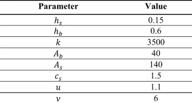
In this section, the numerical analysis of the equations obtained in sections 3 and 5 are presented. The values for input parameters are given in Table 1 (as given in Esmaeili, 2009). We also set the values of between 1 and 2 with steps of 0.1. The optimal values of order quantity and retail price,
Table 1 Parameters values
Parameter Value
ℎ 0.15
ℎ 0.6
3500 40 140 1.5 1.1 6
the profit of each parties in both coordinated and non-coordinated chain as well as the contractual parameters, are presented in Table 2.
Table 2 shows that by increasing the value of α, the surplus achieved by chain coordination is
increasing significantly. The percentage of improvement in chain’s income against different values of α, can be observed in Table 3. Having noted the structure of the problem, we can easily justify this trend. The greater value of α, the more price sensitive demand. Therefore, to improve the chain-wide profit, it may be necessary to reduce the retail price more than before to maintain a proper level for the demand. Since reducing the retail price, as the buyer's decision, has negative effect on buyer’s profit, he/she is not willing to make the necessary reduction without a side-payment contract. Sometimes, it is even necessary to set less than in order to achieve the maximum chain-wide profit. For example, in the last four rows of Table 2, ∗ is less than 6, which is the value
of from Table 1. Obviously, without side-payment contract, there is a loss for the buyer, but proper side-payments will compensate this loss and the buyer will agree to reduce the retail price significantly, if a proper profit allocation is suggested by the contract.
Another interesting trend can be observed in Table 2. It is seen that while changing α,
remains almost fixed. In fact, changes just a little, in order of the tenth decimal place. It is shown in section 3 that is the amount that the seller is willing to pay to increase the order quantity by one unit; therefore, it is expectable that changing the price elasticity does not have a significant influence on . Another reason for lack of sensitivity of to α,is the flatness of chain-wide profit function near the optimal quantity, as it can be easily observed from Figures 1 and 2. On the other hand, from table 2, is highly affected by the change in α. In fact, as the importance of price in the
demand realization increases, the amount which the seller is willing to pay to reduce the retail price by one unit increases, so this sensitivity is reasonable.
Table 2Numerical analysis results for seller-buyer supply chain
Before Coordination After Coordination
α ∗ ∗
1.1 72.81 64.61 68.64 2052.93 2121.57 25.48 220.39 118.13 2102.42 2220.55 16.573 0.218 -567.54 1.2 39.17 75.63 108.49 1377.83 1486.31 12.81 283.16 188.83 1458.17 1647.00 61.517 0.218 -1217.84 1.3 28.22 77.91 117.74 965.03 1082.78 8.98 313.96 215.26 1062.55 1277.81 118.27 0.218 -1745.8 1.4 22.83 76.47 111.89 692.43 804.32 7.16 329.74 217.79 798.33 1016.12 177.212 0.218 -2165.95 1.5 20.17 73.97 101.96 537.02 638.98 6.28 335.98 210.24 645.30 855.54 222.30 0.218 -2435.9 1.6 17.54 69.05 83.72 371.44 455.16 5.42 338.51 190.66 478.38 669.05 282.847 0.218 -2743.42 1.7 16.08 64.44 68.11 275.27 343.38 4.94 336.34 170.88 378.04 548.91 325.017 0.218 -2928.05 1.8 15.01 59.68 53.47 204.80 258.27 4.60 331.45 150.26 301.59 451.85 358.79 0.218 -3052.02 1.9 14.20 54.92 40.38 152.62 193.00 4.34 324.53 130.04 242.28 372.32 383.92 0.218 -3120.92
In Figures 1 and 2, the buyer’s income and the total chain’s income for α=1.9, respectively, are
plotted versus lot size. The concavity of the income functions, proved at Appendices, can be easily observed in these figures. All calculations and figures have been prepared by MATLAB 7.4.0 software.
To give an example for the quantity discount contract, suppose that α=1.7, therefore, we have
= = .
. = 0.689. Now, we have the following function which is more easier to implement
than the general side-payment contract:
( , ) = −40+ − 0.689 −180 − 0.0001 . 0.5 + 1.033
Table 3 Improvement percentage in chain-wide profit
α Improvement percentage
1.1 4.665412878 1.2 10.81133815 1.3 18.01196919 1.4 26.33280286 1.5 33.8915146 1.6 46.99226646 1.7 59.85497117 1.8 74.95256902 1.9 92.9119171
An important input parameter on the contract is . In Fig. 3, we can see the effect of demand constant ( ) on the improvement fraction achieved by the contract. As is clear from this figure, the greater , the greater improvement fraction achieved. This effect can be justified in a same way as we did for α: by increasing the influence of retail price on the demand will be increased. Then the
chain-wide income will be multiplied by a greater constant because the changes in retail price. It is shown that increasing the price effect, leads to an increase in improvement achieved by the contract, hence, this trend is justified. However, regarding to Fig. 3, the sensitivity of the contract to is much less than its sensitivity to α, because the relation between and αwith demand are linear and exponential, respectively.
As an example of parameter effects on decision variables, in Fig 4., it can be seen that the buyer’s unit inventory holding cost affects the optimal retail price. In fact, increasing ℎ will lead to an increase in ∗, because their relations are from the order of square root as it was shown by equations (18) and (20).
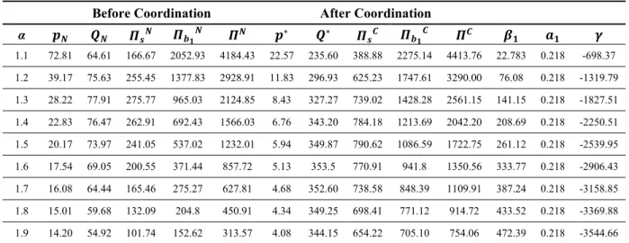
We conclude this section by representing the numerical analysis results for the contract developed
in section 5. The corresponding values of αcome from Table 2. The input parameters for seller and
buyer1 are taken from Table 1 and ℎ = 0.5، = 130 (near to values considered for buyer1)
and = 300 for buyer 2. The results are presented in Table 4.
It can be observed from Table 4 that the values related to buyer1, in non-coordinated chain, are the same as those in Table 2. This was expectable because the income structure of buyer1 and his/her relation with seller, is not affected by introducing buyer 2 to the chain. However, the income structure of the seller is highly affected by this change, as it was seen in Table 4, in form of changing his/her income.
Figure 1 Buyer income vs. lot size, in non-coordinated chain, = 1.9
0 100 200 300 400 500 600
0 20 40 60 80 100 120 140 160
Figure 2 Chain income vs. lot size in coordinated chain, = 1.9
0 500 1000 1500
0 50 100 150 200 250 300 350 400
2000 2200 2400 2600 2800 3000 3200 3400 3600 3800 4000 0.24 0.245 0.25 0.255 0.26 0.265 0.27 0.275
Figure 3 Improvement fraction vs. demand constant, = 1.4 −
0.2 0.3 0.4 0.5 0.6 0.7 0.8 0.9 1
6.4 6.6 6.8 7 7.2 7.4 7.6 7.8 8 ℎ ∗
Figure 4 Optimal retail price vs. unit inventory holding cost, = 1.4
It is also clear that the value is the same as α. We know that this parameter shows the amount that seller is willing to pay to reduce the buyer1 order quantity by one unit. Since there is no possibility to integrate buyers’ orders in this model, this value remains unchanged. Finally, we turn our attention to , the values suggested for this contractual parameter are always higher than those
Table 4 Numerical analysis results for two buyer-single seller chain
Before Coordination After Coordination
α ∗ ∗
1.1 72.81 64.61 166.67 2052.93 4184.43 22.57 235.60 388.88 2275.14 4413.76 22.783 0.218 -698.37 1.2 39.17 75.63 255.45 1377.83 2928.91 11.83 296.93 625.23 1747.61 3290.00 76.08 0.218 -1319.79 1.3 28.22 77.91 275.77 965.03 2124.85 8.43 327.27 739.02 1428.28 2561.15 141.15 0.218 -1827.51 1.4 22.83 76.47 262.91 692.43 1566.03 6.76 343.20 784.18 1213.69 2042.20 208.69 0.218 -2250.51 1.5 20.17 73.97 241.05 537.02 1232.01 5.94 349.87 790.62 1086.59 1722.75 261.12 0.218 -2539.95 1.6 17.54 69.05 200.55 371.44 857.72 5.13 353.5 770.91 941.8 1350.56 333.77 0.218 -2906.43 1.7 16.08 64.44 165.46 275.27 627.81 4.68 352.60 738.58 848.39 1109.91 387.24 0.218 -3158.85 1.8 15.01 59.68 132.09 204.8 450.91 4.34 349.25 698.41 771.12 914.72 433.52 0.218 -3369.88 1.9 14.20 54.92 101.74 152.62 313.57 4.08 344.15 654.22 705.10 754.06 472.39 0.218 -3544.66
suggested in Table 1, for the same α. Since we assume a common retail price for two buyers, a
reduction in this price will result in increasing both demands faced by each buyer. The seller has a demand equal to the sum of these two demands. Therefore, by reducing the retail price, he/she experiences a further increase in the demand, in comparison with a single buyer model. Since the
profit is in direct relation with demand and shows the amount that the seller is willing to pay to
decrease the retail price by one unit, this increase was expectable.
The results obtained from numerical analysis, summarized in figures and tables, in this section; verify the previously stated results about the functions shapes and the improvement achieved by using the contract. Therefore, depending on the input parameters values and the cost of acquiring the required information, this contract can be of great benefit in many settings.
7. CONCLUSION
In this paper, we developed a general side-payment contract for a seller-buyer supply chain. Under this contract, chain operates in its optimal state and due to the proper profit allocation imposed by the contract; both members gain more than the non-cooperative case. We also changed the contract into an easy to implement one, extended it to contain another buyer subject to some assumptions and showed the contract efficiency by numerical analysis.
Several extensions are possible for this model. This model only considers a small part of a supply chain, it seems necessary to extend that to study a chain with more echelons and/or to contain more sellers and buyers; an important special case is when several buyers compete in a common market. In our model, both buyer and seller are risk-neutral; but we know that the attitude of chain members toward risk, affects the negotiation power and so the allocation of profit (Nagarajan and Sosic, 2008). Thus a reasonable extension is to model the chain with members who are not risk-neutral. Another important improvement is to consider the demand as a random variable in this model.
REFERENCES
[1] Breiter A., Hegmanns T., Hellingrath B., Spinler S. (2009), Coordination in Supply Chain Management-Review and Identification of Directions for Future Research, In: Voß S. et al. (eds.); Logistik Management:Systeme, Methoden, Integration, first edition,Physica-Verlag; 1-36.
[2] Cachon G.P. (2003), Supply chain coordination with contracts, In: de Kok A.G., Graves S.C. (Eds.); Supply Chain Management: Design, Coordination and Operation, Elsevier, Amsterdam; 229–340. [3] Carter J.R., Ferrin B.G. (1995), The impact of transportation costs on supply chain management;
Journal of Business Logistics 16 (1); 189–212.
[4] Esmaeili M., Aryanezhad M.B., Zeephongseku P. (2009), A game theory approach in seller–buyer supply chain; European Journal of Operational Research 195; 442-448.
[5] Hezarkhani B., Kubiak W. (2010), Coordinating Contracts in SCM: A Review of Methods and Literature; Decision Making in Manufacturing and Services 4 (1–2); 5–28.
[6] Kanda A., Deshmukh S.G. (2008), Supply chain coordination: perspectives, empirical studies and research directions; International Journal of Production Economics115; 316-335.
[7] Lai G., Debo L.G., Sycara K. (2009), Sharing inventory risk in supply chain: The implication of financial constraint; Omega 37; 811-825.
[8] Lee W.J., Kim D., Cabot A.V. (1996), Optimal demand rate, lot sizing, and process reliability improvement decisions; IIE Transactions 28; 941–952.
[9] Leng M., Parlar M. (2010), Game-theoretic analyses of decentralized assembly supply chains: Non-cooperative equilibria vs. coordination with cost-sharing contracts; European Journal of Operational Research 204; 96-104.
[10] Leng M., Zhu A. (2009), Side-payment contracts in two-person nonzero-sum supply chain games: Review, discussion and applications; European Journal of Operational Research 196; 600-618. [11] Lemaire J. (2008), Cooperative game theory and its insurance applications; ASTIN Bulletin 21 (1);17–
40.
[12] Nagarajan M., Sosic G. (2008), Game-theoretic analysis of cooperation among supply chain agents: Review and extensions; European Journal of Operational Research 187; 719-745.
[13] Prakash L. Abad (1988), Determining optimal selling price and the lot size when the supplier offers all-unit quantity discounts; Decision Sciences 3 (19); 622–634.
[14] Rubin P.A., Carter J.R. (1990), Joint optimality in buyer–supplier negotiations, Journal of Purchasing and Materials Management 26(2); 20–26.
[15] Sarmah S.P., Acharya D., Goyal S.K. (2006), Buyer vendor coordination models in supply chain management; European Journal of Operational Research 175; 1-15.
APPENDICES A(1)
( ( ), )
( ) = 0.5ℎ , substituting from (3) and further simplification results in
= . that is the same as (5).
A(2)
Considering equation (3) we get
= − (A2-1)
from A(1), we have
( ( ), )
= − 0.5ℎ (A2-2)
by (A2-1) and (A2-2), we have ( ( ), )
= (−2 +
− 1( ))
We only need to show that −2 + ( ) < 0 holds. By substitution from (3)
−2 + = + ( ), which is always negative, given the assumption 1 < < 2.
A(3)
Substituting (3) into (5), we obtain
= 2
ℎ × ( − 1) × +
setting = × ( ) and rearranging results as
× =
Now, by assuming = and = , we come to the following equation which can be easily
solved numerically
× − = 0, the resulted can be used to calculate from (3).
Similar to A (1), we have
( ∗( ), )
= × ∗ ∗ − ∗ + ∗ − 0.5(ℎ + ℎ ) = 0
∗ (
∗
) = 0.5(ℎ + ℎ )
substituting from (18) and further simplification yields
∗= ∗
( ) , that is the same as (20).
A(5)
Using the same procedure as A (2), we obtain Π( ∗( ), Q)
= ∗
(−2 ∗+
− 1( ))
Now, it is enough to show that: −2 ∗+ ( ) < 0, substituting from (18) and simplification
yields −2 ∗+ = + ( ) , referring to the assumption 1 < < 2, this is always
negative.
A(6)
Substituting from (18) into (20) and simplification yields
∗= 2
(ℎ + ℎ )× ( − 1) × + ∗
Now, assume = ( )× ( ) , rearranging results as
∗ × ∗ =
if we put: = and = , then, we obtain the following equation
∗ × ∗ − = 0
This equation can be solved numerically and the resulted ∗ can be used to compute ∗from