Sharif University of Technology
Scientia IranicaTransactions A: Civil Engineering http://scientiairanica.sharif.edu
Predicting the eective stress parameter of unsaturated
soils using adaptive neuro-fuzzy inference system
H. Rahnema
a;, M. Hashemi Jokar
a;1, and H. Khabbaz
ba. Department of Civil and Environmental Engineering, Shiraz University of Technology, Shiraz, Iran. b. School of Civil and Environmental Engineering, University of Technology, Sydney (UTS).
Received 7 March 2017; received in revised form 29 August 2017; accepted 19 February 2018
KEYWORDS Unsaturated soils; Eective stress parameter; ANFIA;
Fuzzy clustering; Subtractive clustering; FCM clustering.
Abstract. The eective stress parameter () is applied to obtain the shear strength of unsaturated soils. In this study, two Adaptive Neuro-Fuzzy Inference System (ANFIS) models, including SC-FIS model (created by subtractive clustering) and FCM-FIS model (created by Fuzzy c-means (FCM) clustering), are presented for prediction of , and the results are compared. The soil-water characteristic curve tting parameter (), the conning pressure, the suction, and the volumetric water content in dimensionless forms are used as input parameters for these two models. By using a trial-and-error process, a series of analyses were performed to determine the optimum methods. The ANFIS models were constructed, trained, and validated to predict the value of . The quality of the ANFIS prediction ability was quantied in terms of the determination coecient (R2),
Root Mean Square Error (RMSE), and Mean Absolute Error (MAE). These two ANFIS models are able to eectively predict the value of with reasonable values of R2, RMSE,
and MAE. Sensitivity analysis was implemented to determine the eect of input parameters on prediction, and the results revealed that the conning pressure and the volumetric water content parameters had the most inuence on prediction.
© 2019 Sharif University of Technology. All rights reserved.
1. Introduction
Compacted soils, which are commonly used in geotech-nical engineering projects, such as earth dams, high-ways, embankments, and airport runhigh-ways, are mostly unsaturated. To achieve a safe design in all these projects, the stress state variable in soil plays a sig-nicant role. Any proposed model for the stress state variable should express its independence from the soil
1. Present address: Graduate University of Advanced Technology, Kerman, Iran.
*. Corresponding author. Tel/Fax: +98 713 7277656 E-mail addresses: [email protected] (H. Rahnema); [email protected] (M. Hashemi Jokar); [email protected] (H. Khabbaz)
doi: 10.24200/sci.2018.20200
properties [1]. In saturated soils, the eective stress is taken into account as the stress state variable [2]. Some researchers have attempted to nd the stress state variable for unsaturated soils the same as that for saturated soils with only one variable; however, they have noticed that the soil properties have been involved in the proposed models [3-6]. Therefore, in unsaturated soil, the stress state variable consists of two stress state variables [4]:
0= ( u
a) + (ua uw); (1)
where is the eective stress parameter. Parameter varies from 1 to 0 from saturated to dry soils, respectively, ua is the pore air pressure, ( ua) is the
net normal stress, and (ua uw) is the matric suction
denoted by S. Khalili and Khabbaz [7] solved as a function of suction ratio as follows:
= 8 < :
ua uw
ue
0:55
for ua uw> ue
1 for ua uw ue
(2) where ue(the air entry value) is a measure of suction,
showing the transition from the saturated state to the unsaturated state. Determining all of these parameters to quantify the value of is a dicult and time-consuming task and needs conducting many laboratory tests. In addition, theoretical studies have also shown that is highly nonlinear and may exceed unity [8].
The shear strength of unsaturated soil may be determined by means of the concept of the stress state variable. Bishop [4] proposed the following equation to calculate the shear strength of unsaturated soils:
= c0+ ( u
a) tan 0+ S tan 0; (3)
where c0 and 0 are the eective cohesion and the
internal friction angle, respectively.
According to the shear strength of saturated soils, Eq. (3) is presented by Fredlund et al. [9] to calculate the shear strength of unsaturated soils.
= c0+ ( u
a) tan 0+ S tan b; (4)
where b is the friction angle associated with changes
in S alone. The relationship between 0 and b is
presented by Escario and Saez [10] as follows: = tan b
tan 0: (5)
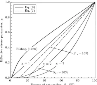
is generally assumed to be a function of the degree of saturation (Sr). This parameter has been proposed
through the best-t regression formulas conducted on some suitable experimental data. In the following equations, is presented as a function of Sr, which
is obtained from the best t of the experimental results [11,12]:
= Sk r =
s
k
; (6)
= Sr Srr
1 Srr =s rr; (7)
where Srr is the residual degree of saturation (the
saturation of water around the soil particle surfaces exists like tine lms), Sr is the degree of saturation
(at the moment of testing), , s, and r are the
volumetric, saturated, and residual volumetric water contents, respectively, and k is an optimized parameter, determined from the best t between measured and predicted values. Figure 1 shows Sr versus for the
various values of k and Srr [8].
An accurate prediction of can be achieved when improved approaches are utilized for a nonlinear
Figure 1. Sr versus for various values of k and Srr[8].
problem. Articial Intelligence (AI) based techniques have been useful as an alternative approach to replace the conventional techniques for the prediction of engi-neering problems. Some AI-based models have been recently used for the prediction of based on available empirical data [13-15].
Due to the nonlinearity of the relationship be-tween and related parameters, the prediction process can be complex. Therefore, a powerful model, such as the Adaptive Neuro-Fuzzy Inference System (ANFIS) model, should be employed to predict the process ac-curately. ANFIS models are well-known hybrid neuro-fuzzy networks for modeling complex systems [16]. Characterized by the learning capability from past experiences, ANFIS is going to be one of the pillars of scientic research [17].
In the eld of geotechnical engineering, the use of ANFIS is also in progress. Gokceoglu et al. [18] used the neuro-fuzzy system to estimate the defor-mation modulus of rock masses, and their neuro-fuzzy model exhibited a high performance. Kalkan et al. [19] developed ANFIS and Articial Neural Network (ANN) models to predict the Unconned Compressive Strength (UCS) of compacted granular soils, and the results of the ANFIS model were very encouraging, compared to the ANN model. Kayadelen et al. [20] used ANFIS to predict the swell percentage of compacted soils, and showed that ANFIS was a more reasonable method for predicting the swelling potential of soils. Cobaner [21] predicted the estimation of evapotranspiration (ET0) using climatic variables by two ANFIS models, based on grid partition (G-ANFIS) and subtractive clustering (S-ANFIS), and Multi-Layer Perceptron (MLP) model; it was found that S-ANFIS model showed better results than G-ANFIS and MLP models. Sezer et al. [22] successfully trained an ANFIS model to predict permeability based on 20 dierent
types of granular soils. Ikizler et al. [23] showed that neural network and adaptive neuro-fuzzy-based prediction models could satisfactorily be used to obtain the swelling pressure of expansive soils. Doostmoham-madi [24] used ANFIS model to predict time-dependent swelling pressure (SPf), compared the ANFIS results with ANN and multiple regression approaches, and proved that the ANFIS model was more eective in modeling the cyclic swelling pressure. Cabalar et al. [25] developed ANFIS models for (I) damping ratio and shear modulus of coarse rotund sand-mica mix-tures based on experimental results from Stokoe's res-onant column testing apparatus, (II) deviatoric stress-strain, pore water pressure generation-strain properties of coarse rotund sand-mica mixtures from triaxial testing apparatus, and (III) liquefaction triggering. Zoveidavianpoor [26] compared the capability levels of ANN and ANFIS for the prediction of compressional wave (p wave) velocity, and proved that ANFIS and ANN systems performed comparably well and accurate for the prediction of p wave.
2. Adaptive Neuro-Fuzzy Inference System (ANFIS)
Fuzzy Logic (FL), introduced by Zadeh [27], is com-monly applied with investigative knowledge and im-precise inputs to realize complicated functions. The membership grade with the numbers 0 or 1 is expressed in the classical logic; however, FL can have any number between 0 and 1. Membership grade of each member is determined by the membership functions. Fuzzy Inference System (FIS) is the same as a black box, which connects the input space to the output space through some fuzzy if-then rules. A fuzzy if-then rule can be shown as follows:
if x is A then y is B;
where A and B are linguistic values dened by fuzzy sets on the ranges (universes of discourse) X and Y , respectively. \x is A" is called antecedent or premise, and \y is B" is called consequent or conclusion [28]. Three well-known FIS models include Mamdani and Assilian [29], Takagi-Sugeno-Kang (TSK) [30], and Tsukamoto [31].
Neural Networks (NNs) [32] can learn from his-torical data and train themselves to achieve high per-formance, while extensive expertise is not mandatory. Among the most powerful data-driven methods, FL and NNs systems are able to monitor data pattern classication in diagnostic tasks. Adaptive Neuro-Fuzzy Inference System (ANFIS) [16] is a combination of FL and NNs. ANFIS applied a Takagi-Sugeno-Kang Fuzzy Inference System (TSK-FIS) to a set of input and output data. TSK-FIS if-then rules are simply presented as follows [33]:
Figure 2. A typical fuzzy model of TS type [16].
Figure 3. A typical ANFIS structure [58].
Rule 1 : if x is A1; y is B1then f1= p1x + q1y + r1;
Rule 2 : if x is A2; y is B2then f2= p2x + q2y + r2;
where Ai and Bi are the linguistic labels of the ith
rule. pi, qi, and ri are the consequent parameters in
the TSK-FIS [28].
TSK-FIS with 2 inputs (x and y) and one output (f) is presented in Figure 2.
ANFIS, as an optimization method, uses hybrid learning algorithms (gradient descent and least-squares method). The antecedent and consequent parameters will be adjusted with gradient descent and least-squares method, respectively [33]. Figure 3 shows the ANFIS structure that has ve layers of nodes including square nodes (adaptive nodes whose parameters will vary during training) and circle nodes (xed nodes whose parameters will not vary during training).
The layers of ANFIS are described as follows [16]:
In Layer 1, the fuzzy membership grade of the inputs may be obtained through Eq. (8) as follows:
O1;i= Ai(x) i = 1; 2;
O1;i= B(i 2)(x) i = 3; 4; (8)
where Ai and Bi are the grades of membership
functions of Aiand Bi, respectively, and are dened
by the membership function;
In Layer 2, the output of each node is multiplied by the input signals and represents the ring strength (the degree that the antecedent part of a fuzzy rule
is fullled) of a law.
O2;i= wi= Ai(x) Bi(y) i = 1; 2; (9)
where wi is the ring strength of the ith rule.
In Layer 3, the normalized ring strength, wi, is
presented as follows: O3;i= wi= w wi
1+ w2: (10)
In Layer 4, the contribution of the ith rule in the output is calculated with an adaptive function:
O4;i= wifi = wi(pix + qiy + ri) ; (11)
where fi is the linear function of the inputs.
Finally, in Layer 5, the summation of all input signals is calculated as follows:
O5;i=
X
iwifi=
P
iwifi
P
iwi : (12)
In this paper, to determine the membership grade, the Gaussian membership function is used as follows:
Ai(xj) = e
xj cji ji
2
; (13)
where xj is the input data variable; cji and ji are the
center (mean) and the width (standard deviation) of the membership function, respectively. Actually, cji and ji are the antecedent parameters of fuzzy rules for the Gaussian membership function.
3. Fuzzy clustering
Fuzzy clustering of data provides a division of the data space into fuzzy clusters and gives useful information by grouping data from a large dataset that represents a system behavior. In this way, each obtained cluster center represents a rule. There are several methods for clustering such as k-means clustering [34], fuzzy c-means clustering [35], and mountain and subtrac-tive clustering method, which is a non-iterasubtrac-tive algo-rithm [36]. In this paper, the initial FIS for ANFIS models is used, which is created by subtractive and fuzzy c-means clustering methods.
3.1. Subtractive clustering
In 1994, the Subtractive Clustering (SC) model was developed by Chiu [36,37]. This model is a fast, robust, and accurate algorithm for specifying the number of clusters and the cluster centers in a set of data. SC is an extension of the grid-based mountain clustering method [38]. Based on the density of surrounding data points, in the SC method, each data point is assumed to be a likely cluster center, and its potential is then calculated. The steps of the SC process for a collection of n data points, Y = fy1; y2; : : : ; yng, in d-dimensional
space can be summarized as follows [36]:
1. Normalize the dataset between 0 and 1 by calculat-ing the followcalculat-ing formulation for each dimension of data:
xl
i= y
l i ylmin
yl
max ylmin
i = 1; 2; :::; n l = 1; 2; :::; d; (14) where xl
i is the normalized value of the ith data
in the lth dimension, yl
i is the ith data in the lth
dimension, and yl
min and ymaxl are the minimum
and maximum values of data samples in the lth dimension.
2. Determine a potential value at each data point, xi:
pi= n
X
j=1
e kxi xjk2; (15)
= r42
a; (16)
where jj:jj is the Euclidean distance, xi and xj
are the normalized data points with d-dimensional space, and rais the positive constant between 0 and
1, representing a neighborhood radius.
The data points with many neighboring data points will have high potential value. The rst cluster center is chosen as the data point with the maximum potential value among all other data points;
3. Calculate the reduction potential value of each remaining data point as follows:
pi= pi p1e kxi x
1k2; (17)
= 4 r2
b; (18)
rb= ra; (19)
where x
1is the rst cluster center, p1is its potential
value, and is the squash factor with a constant value greater than 1.
The second cluster center is chosen as a data point with the maximum remaining potential;
4. Find the other cluster centers using the following equation:
pi= pi pke kxi x
kk2; (20)
where x
c is the kth cluster center, and pk is its
potential value data as a cluster center. Some conditions, such as Eqs. (21) to (23), must be checked in the SC process [33]:
p
k > "p1; (21)
p
dmin
ra +
p k
p
1 1; (23)
where " and " are accepted and rejected ratios, re-spectively, and dminis the shortest distance between
x
k and all the previously found cluster centers. xk,
as a cluster center, will be accepted, when Eq. (21) is satised; the clustering process will be completed if Eq. (22) is satised; consequently, Eq. (23) should be satised. Chiu [36] suggested that " = 0:5 and " = 0:15. The fourth step will be repeated until the above conditions are fullled and, then, the SC process is accomplished. The number of clusters and fuzzy rules is equal and will be changed by the value of ra. The great value of ra makes a fewer
number of cluster centers, and vice versa [33]. 3.2. Fuzzy c-means clustering
Fuzzy c-means (FCM) clustering was developed by Dunn [39] and improved by Bezdek [35]. In the FCM clustering, rstly, the number of clusters is chosen, and the sample data points are clustered into the chosen cluster numbers. This method can obtain the cluster centers directly. Let Y = fy1; y2; : : : ; yng be
the sample data points, and each data point has d-dimensions. These data points should be clustered into C clusters. The objective function for FCM is dened as follows:
Jm= n X i=1 c X j=1 um
ijkyi cjk2; (24)
where m is the weighting exponent and has a constant value greater than 1. Bezdek [35] suggested that m = 2, yi is the ith data point, cj is the jth center of cluster,
jj:jj is the Euclidean distance between yi and cj, and
uij is the membership degree of the ith data point in
the jth cluster.
uij and cj are calculated by the following
equa-tions [33]:
uij =P 1 c k=1
kyi cjk
kyi ckk
2
m 1; (25)
c = Pn
i=1umij yi
Pn
i=1umij ; (26)
In the clustering process, Eqs. (25) and (26) will be updated until the stopping condition (Eq. (27)) is fullled.
maxnu(k+1)ij u(k)ij o< "; (27) where " is a criterion value to stop clustering, and k is the iteration step.
The above formulation allows the objective func-tion (Jm) to converge to the possible minimum
value [33].
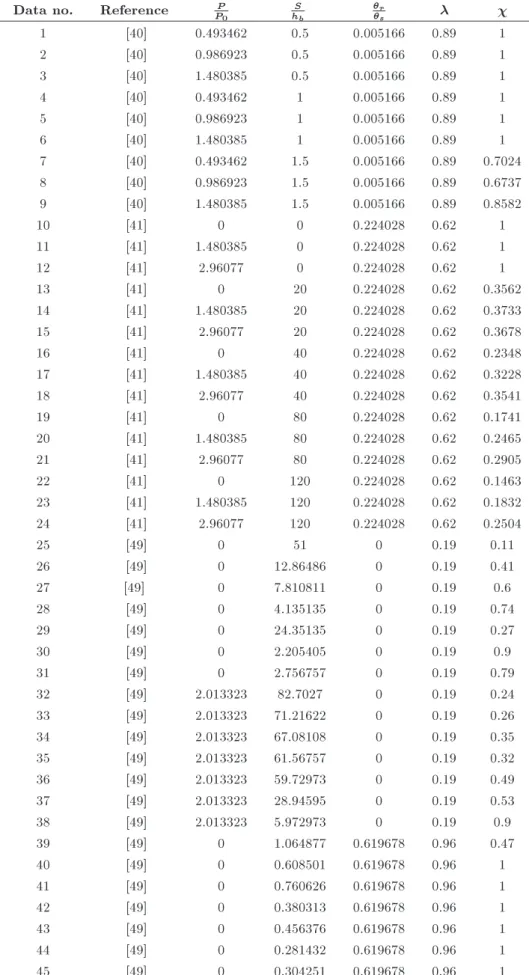
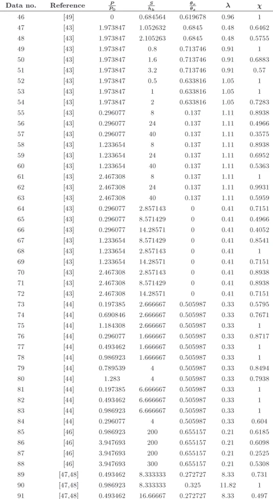
4. Used database for modeling
In this study, the datasets used to develop two ANFIS models were derived from 120 collected data from the literature [40-49]. These data were associated with the results of triaxial, shear, pressure plate, and lter paper tests. These datasets consist of seven characteristics of unsaturated soils: suction (S), bubbling pressure (hb), net conning pressure (P ), residual water content
(r), saturated volumetric water content (s),
soil-water characteristic curve tting parameter (), and eective stress parameter (). S, hb, P , r, and s
characteristics of data became dimensionless as follows:
P
P0 is the dimensionless conning pressure parameter
P0 = 101:325 kPa, hSb is the dimensionless suction
parameter, and r
s is the dimensionless volumetric
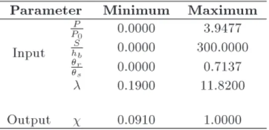
water content parameter (Table 1). Table 2 shows the range of P
P0,
S hb,
r
s, and .
The datasets were divided into three separate groups: the training dataset (used to train the ANFIS model) by 85 data (71%), the validation dataset (used to prevent overtting through training procedure) by 15 data (12%), and the testing dataset (used to verify the accuracy and eectiveness of the model) by 20 data (17%). The data were chosen randomly in each dataset. 5. Developing ANFIS models to predict
value
In order to develop the ANFIS model, rstly, the initial Fuzzy Inference System (FIS) was created and, then, trained by ANFIS. In this paper, two initial FIS models, SC-FIS and FCM-FIS, were created by the application of Subtractive Clustering (SC) and Fuzzy c-means (FCM) clustering, respectively. In other words, the TSK-FIS in these models was created by the SC and FCM clustering, respectively. The fuzzy if-then rules in TSK-FIS models for predicting are dened as follows: Rulec : 8 > > > > > > < > > > > > > :
If x1 is A1c and x2 is A2c and x3is A3c
and x4is A4c
Then fc = p0c+ p1cx1+ p2cx2
+p3cx3+ p4cx4
where x1, x2, x3, and x4 are hSb, PP0, rs, and ,
respectively. c is the cluster number (c = 1 C), A1c; A2c, A3c, and A4c are the linguistic labels (the
fuzzy membership functions) of the cth rule, fc is the
consequent of Rule c, and p0c, p1c, p2c, p3c, and p4c
are the consequent parameters for the cth rule. As mentioned earlier, the number of the clusters is equal to that of fuzzy rules and membership functions. To achieve the best solution to the problem with high
Table 1. The dimensionless data used for modeling . Data no. Reference P
P0
S hb
r
s
1 [40] 0.493462 0.5 0.005166 0.89 1
2 [40] 0.986923 0.5 0.005166 0.89 1
3 [40] 1.480385 0.5 0.005166 0.89 1
4 [40] 0.493462 1 0.005166 0.89 1
5 [40] 0.986923 1 0.005166 0.89 1
6 [40] 1.480385 1 0.005166 0.89 1
7 [40] 0.493462 1.5 0.005166 0.89 0.7024
8 [40] 0.986923 1.5 0.005166 0.89 0.6737
9 [40] 1.480385 1.5 0.005166 0.89 0.8582
10 [41] 0 0 0.224028 0.62 1
11 [41] 1.480385 0 0.224028 0.62 1
12 [41] 2.96077 0 0.224028 0.62 1
13 [41] 0 20 0.224028 0.62 0.3562
14 [41] 1.480385 20 0.224028 0.62 0.3733
15 [41] 2.96077 20 0.224028 0.62 0.3678
16 [41] 0 40 0.224028 0.62 0.2348
17 [41] 1.480385 40 0.224028 0.62 0.3228
18 [41] 2.96077 40 0.224028 0.62 0.3541
19 [41] 0 80 0.224028 0.62 0.1741
20 [41] 1.480385 80 0.224028 0.62 0.2465
21 [41] 2.96077 80 0.224028 0.62 0.2905
22 [41] 0 120 0.224028 0.62 0.1463
23 [41] 1.480385 120 0.224028 0.62 0.1832
24 [41] 2.96077 120 0.224028 0.62 0.2504
25 [49] 0 51 0 0.19 0.11
26 [49] 0 12.86486 0 0.19 0.41
27 [49] 0 7.810811 0 0.19 0.6
28 [49] 0 4.135135 0 0.19 0.74
29 [49] 0 24.35135 0 0.19 0.27
30 [49] 0 2.205405 0 0.19 0.9
31 [49] 0 2.756757 0 0.19 0.79
32 [49] 2.013323 82.7027 0 0.19 0.24
33 [49] 2.013323 71.21622 0 0.19 0.26
34 [49] 2.013323 67.08108 0 0.19 0.35
35 [49] 2.013323 61.56757 0 0.19 0.32
36 [49] 2.013323 59.72973 0 0.19 0.49
37 [49] 2.013323 28.94595 0 0.19 0.53
38 [49] 2.013323 5.972973 0 0.19 0.9
39 [49] 0 1.064877 0.619678 0.96 0.47
40 [49] 0 0.608501 0.619678 0.96 1
41 [49] 0 0.760626 0.619678 0.96 1
42 [49] 0 0.380313 0.619678 0.96 1
43 [49] 0 0.456376 0.619678 0.96 1
44 [49] 0 0.281432 0.619678 0.96 1
Table 1. The dimensionless data used for modeling (continued). Data no. Reference P
P0
S hb
r
s
46 [49] 0 0.684564 0.619678 0.96 1
47 [43] 1.973847 1.052632 0.6845 0.48 0.6462
48 [43] 1.973847 2.105263 0.6845 0.48 0.5755
49 [43] 1.973847 0.8 0.713746 0.91 1
50 [43] 1.973847 1.6 0.713746 0.91 0.6883
51 [43] 1.973847 3.2 0.713746 0.91 0.57
52 [43] 1.973847 0.5 0.633816 1.05 1
53 [43] 1.973847 1 0.633816 1.05 1
54 [43] 1.973847 2 0.633816 1.05 0.7283
55 [43] 0.296077 8 0.137 1.11 0.8938
56 [43] 0.296077 24 0.137 1.11 0.4966
57 [43] 0.296077 40 0.137 1.11 0.3575
58 [43] 1.233654 8 0.137 1.11 0.8938
59 [43] 1.233654 24 0.137 1.11 0.6952
60 [43] 1.233654 40 0.137 1.11 0.5363
61 [43] 2.467308 8 0.137 1.11 1
62 [43] 2.467308 24 0.137 1.11 0.9931
63 [43] 2.467308 40 0.137 1.11 0.5959
64 [43] 0.296077 2.857143 0 0.41 0.7151
65 [43] 0.296077 8.571429 0 0.41 0.4966
66 [43] 0.296077 14.28571 0 0.41 0.4052
67 [43] 1.233654 8.571429 0 0.41 0.8541
68 [43] 1.233654 2.857143 0 0.41 1
69 [43] 1.233654 14.28571 0 0.41 0.7151
70 [43] 2.467308 2.857143 0 0.41 0.8938
71 [43] 2.467308 8.571429 0 0.41 0.8938
72 [43] 2.467308 14.28571 0 0.41 0.7151
73 [44] 0.197385 2.666667 0.505987 0.33 0.5795
74 [44] 0.690846 2.666667 0.505987 0.33 0.7671
75 [44] 1.184308 2.666667 0.505987 0.33 1
76 [44] 0.296077 1.666667 0.505987 0.33 0.8717
77 [44] 0.493462 1.666667 0.505987 0.33 1
78 [44] 0.986923 1.666667 0.505987 0.33 1
79 [44] 0.789539 4 0.505987 0.33 0.8494
80 [44] 1.283 4 0.505987 0.33 0.7938
81 [44] 0.197385 6.666667 0.505987 0.33 1
82 [44] 0.493462 6.666667 0.505987 0.33 1
83 [44] 0.986923 6.666667 0.505987 0.33 1
84 [44] 0.296077 4 0.505987 0.33 0.604
85 [46] 0.986923 200 0.655157 0.21 0.6185
86 [46] 3.947693 200 0.655157 0.21 0.6098
87 [46] 3.947693 200 0.655157 0.21 0.2525
88 [46] 3.947693 300 0.655157 0.21 0.5308
89 [47,48] 0.493462 8.333333 0.272727 8.33 0.731
90 [47,48] 0.986923 8.333333 0.325 11.82 1
Table 1. The dimensionless data used for modeling (continued). Data no. Reference P
P0
S hb
r
s
92 [47,48] 0.986923 16.66667 0.325 11.82 0.694
93 [47,48] 0.493462 33.33333 0.272727 8.33 0.239
94 [47,48] 0.986923 33.33333 0.325 11.82 0.337
95 [47,48] 0.493462 66.66667 0.272727 8.33 0.091
96 [47,48] 0.986923 66.66667 0.325 11.82 0.155
97 [45] 0 6.382979 0.066577 0.73 0.4801
98 [45] 0 4.255319 0.066577 0.73 0.6481
99 [45] 0 2.12766 0.066577 0.73 0.9762]
100 [45] 0.493462 4.444444 0.168462 0.94 0.9069 101 [45] 0.493462 5.740741 0.168462 0.94 0.8053 102 [45] 0.493462 9.481481 0.168462 0.94 0.5376 103 [45] 0.986923 3.037037 0.168462 0.94 0.9953 104 [45] 0.986923 4.444444 0.168462 0.94 0.9335 105 [45] 0.986923 5.740741 0.168462 0.94 0.7744 106 [45] 0.986923 8.962963 0.168462 0.94 0.5621 107 [45] 1.480385 4.555556 0.168462 0.94 0.7937 108 [45] 1.480385 5.740741 0.168462 0.94 0.7434 109 [45] 1.480385 9.259259 0.168462 0.94 0.5313
110 [45] 1.973847 2.962963 0.168462 0.94 1
111 [45] 1.973847 5.592593 0.168462 0.94 0.7737 112 [45] 1.973847 8.962963 0.168462 0.94 0.5687 113 [45] 2.467308 2.962963 0.168462 0.94 0.8802 114 [45] 2.467308 4.444444 0.168462 0.94 0.8268
115 [45] 2.467308 5.481481 0.168462 0.94 0.811
116 [45] 2.467308 9.074074 0.168462 0.94 0.5748
117 [45] 2.96077 2.814815 0.168462 0.94 0.9265
118 [45] 2.96077 4.444444 0.168462 0.94 0.8002
119 [45] 2.96077 5.481481 0.168462 0.94 0.8218
120 [45] 2.96077 8.814815 0.168462 0.94 0.5715
Table 2. The range of datasets. Parameter Minimum Maximum
Input
P
P0 0.0000 3.9477
S
hb 0.0000 300.0000
r
s 0.0000 0.7137
0.1900 11.8200
Output 0.0910 1.0000
accuracy and optimize the clustering and training time consumption, nding the appropriate number of fuzzy rules is very important. A number of methods have been recommended to gain the optimum number of clusters such as the cluster validity measure [35,50,51], the compatible cluster merging [52,53], and the trial-and-error method by minimizing the prediction
er-ror [54]. In addition, the overtting may occur in the training process if the number of training epochs is not selected in the appropriated range, leading to misleading results [55].
The accuracy and performance evaluation of SC-FIS and FCM-SC-FIS models should be veried by testing datasets for their rst appearance in ANFIS models. Performance indices such as the determination coe-cient (R2), the Mean Absolute Error (MAE), and the
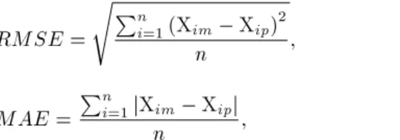
Root Mean Square Error (RMSE) were calculated to assess the accuracy of SC-FIS and FCM-FIS models. These performance measures are presented in Eqs. (28) to (30):
R2=
Pn
i=1XimXip
qPn
i=1Xim2
Pn
i=1Xip2
RMSE = sPn
i=1(Xim Xip)2
n ; (29)
MAE = Pn
i=1jXim Xipj
n ; (30)
where n is the number of data in each dataset, Xim is
the measured value, and Xip is the predicted value.
In the following sections, to predict parameter , the process of nding the optimum number of training epochs and fuzzy rules along with some other key features of the two ANFIS models is presented. 5.1. SC-FIS model
The initial FIS of SC-FIS model was created by SC. In order to determine the best epoch of training ANFIS, some FIS models were created by SC with a range of ra
between 0.1 and 1 and the random choice of Training, Validation, and Testing (TVT) datasets. Other SC chosen parameters include = 1:25, " = 0:5, and " = 0:15. Then, the number of epochs for training was set to 1000. In each epoch, the RMSE was calculated for training and validation sets as an error tolerance. When the designated epoch number was reached, the
error tolerance was plotted. Some error tolerance plots were tried in dierent raand random datasets. Figure 4
represents the plots of four examples of error tolerance for training and validation datasets. In Figure 4(a) and (b), after about 200 epochs, the error tolerance nearly gets constant, and no considerable decrease occurs. As shown in Figure 4(c), overtting occurs after about 400 epochs. Figure 4(d) is an example of when the overtting occurs in the initial epochs and the training is not good; then, in order to prevent overtting, the TVT datasets can be randomly chosen, and the appropriate dataset is obtained to train the model. The best number of epochs for the training process is about 200 to 300 epochs, and it is normally enough for the training process.
The value of ra strongly aects the number of
fuzzy clusters. As raincreases, the fuzzy rules decrease,
and vice versa. Therefore, nding the best ra is
very important for achieving a suitable solution to the problem. To get the best rain SC-FIS model, the
trial-and-error method is used and the code is written in MATLAB software with the following conditions.
The TVT datasets were created randomly, and the range of ra was chosen between 0.1 and 1. This
Figure 4. Examples of the number of epochs versus error tolerance for training and validation datasets for the fuzzy model with the initial SC-FIS model.
range was divided into 25 intervals. The initial FIS was created at each ra interval, and the number of
clusters corresponding to ra intervals was determined.
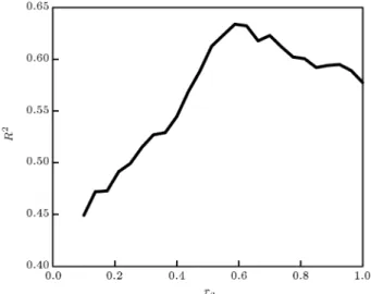
Then, the initial FIS was trained with an epoch equal to 300. For each ra, R2 value was calculated for
the TVT datasets. The above steps were repeated for the specied iterations. For each ra interval, the
average of all R2s and cluster numbers was calculated
and obtained in each iteration corresponding to the ra interval. The ra versus average R2 is plotted in
Figure 5. As can be seen in Figure 5, R2 has the
highest value when ra is determined to be between 0.5
and 0.65. Figure 6 shows the ra versus the number of
clusters. As can be seen in this gure, an increase in ra
decreases the number of clusters. Figure 7 shows the number of clusters versus R2 for SC. In the range of
ra= 0:5 0:65, there are 5 to 10 clusters.
After nding a proper range of ra, the SC-FIS
model was developed to predict value. For this purpose, SC parameters were chosen as follows: = 1:25, " = 0:5, and " = 0:15, ra = 0:5 0:65 by
Figure 5. Variable raversus average R2.
Figure 6. Variable raversus the number of clusters.
Figure 7. Number of clusters versus R2.
dividing into 25 intervals, epoch = 300, and initial R2
= 0. The TVT datasets were randomly created. For each ra interval, the initial FIS was also created and
trained by ANFIS; accordingly, the value of R2 was
calculated for the TVT and the total dataset. Then, the new R2 for the total dataset was compared to
the previous R2. If R2 was greater than the previous
R2, the ANFIS was stored and, then, continued at
the next ra interval. After nishing all ra intervals,
the next iteration and the other TVT dataset were randomly selected, and the above process was repeated. This process continued until the model was not able to nd any greater R2. The best R2 for the
SC-FIS model was found in ra = 0:55 with 9 rules.
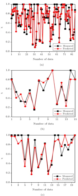
The membership functions before and after training are shown in Figure 8 for the SC-FIS model. The comparison results of the predicted and measured values for the TVT datasets are shown in Figure 9(a) to (c). The measured versus predicted values and, also, the line by R2 = 1 for the TVT datasets are
shown in Figure 10(a) to (c). As can be seen in these gures, there is good agreement between measured and predicted values obtained by the SC-FIS model in the training, validation, and testing datasets.
5.2. FCM-FIS model
The initial FIS of the FCM-FIS model was created by the FCM clustering. In order to assign a proper epoch according to the random TVT datasets, a number of FIS models were created by the FCM clustering, and the number of epochs for training was adjusted to 1000. Figure 11 shows four error tolerance examples in epochs for training and validation datasets by the FCM clustering and initial FIS. As can be seen in Figure 11(a) to (c), after about 100 to 200 epochs, the error tolerance reaches a plateau. This situation was also considered in many other error tolerance gures for various ANFIS training models. Figure 11(d) is an
Figure 8. The membership functions: (a) Before and (b) after training for SC-FIS model.
example of overtting (after about 200 epochs). The number of epochs for the model by the initial FCM-FIS is assumed as 200 epochs.
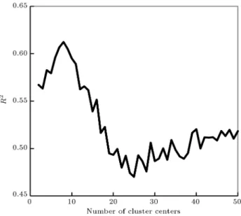
In order to determine the best number of clusters, a MATLAB code was written and used. In this code, for each iteration, the number of clusters was taken to be between 2 and 50, and the data points for the TVT datasets were selected randomly from the total dataset. Then, for each number of cluster intervals, the initial FIS was created and trained by ANFIS with 200 epochs. R2 was calculated according to each
number of cluster intervals. After reaching the last interval of clusters, the next iteration should start; then, the TVT datasets are selected randomly, and these steps are repeated. Following the termination of the desired iteration of selecting random datasets,
the average value of R2 was calculated for each cluster
interval. Then, the number of cluster intervals was plotted versus average R2. Next, the range of the best
number of clusters was selected according to the highest R2. Figure 12 shows the number of clusters versus R2.
According to Figure 12, R2 has the highest value in 7
to 10 clusters.
To develop the FCM-FIS model, a MATLAB code was written. The number of clusters was chosen to be between 7 and 10. For the rst iteration, it was assumed that R2 = 0 and the epoch was taken to
be 200. For each cluster interval, TVT datasets were created randomly, and the initial FIS was created by the FCM clustering and trained by ANFIS. The value of R2 was calculated according to TVT and total
Figure 9. Comparison of the predicted values by SC-FIS model for (a) training, (b) validation, and (c) testing datasets.
compared with the previous R2. If R2 was greater
than the previous R2, the ANFIS was stored and, then,
continued at the next number of cluster intervals. After completing all cluster intervals, other TVT datasets were randomly selected, and the process above was repeated. This process continued until the model failed to nd any greater R2. The FCM-FIS model
found the best R2 in 9 clusters. The membership
Figure 10. The measured versus predicted values by SC-FIS model and, also, the line by R2= 1 for (a)
training, (b) validation, and (c) testing dataset.
functions before and after training of the FCM-FIS model are shown in Figure 13. A comparison of the predicted and measured values for the TVT datasets is represented in Figure 14(a) to (c). The measured versus the predicted values and the line by R2= 1 for
training, validation, and testing datasets are plotted in Figure 15(a) to (c), respectively.
6. Sensitivity analysis
Figure 11. Four examples of the most observed samples of the number of epochs versus error tolerance for training and validation datasets for the fuzzy model with the initial FCM-FIS model.
Figure 12. Number of clusters versus R2.
on value, sensitivity analysis was conducted for all major input parameters. The Cosine Amplitude Method (CAM) [56] was used to obtain the relationship between inputs and outputs. Hence, matrix Z that
contains the data points is considered as follows: 8
> > > < > > > :
Z = fZ1; Z2; :::; Zng
Zk = fzIkzOkg k = 1; 2; :::; n
zIk = fzk1; zk2; :::; zkmg
zOk= fzk1; zk2; :::; zkog
(31) where n is the number of data points; for each data point, zIk is the input vector with lengths of m, ZOk
is the output vector with a length of o, and Zk is the
vector with a length of m + o. In other words, the dataset can be represented by n data points in m + o dimensional space.
rij is considered as the relative inuence of each
input on each output: rij =
n
P
k=1zkizkj
s
n
P
k=1z 2 ki
n
P
k=1z 2 kj
i = 1; 2; :::; m j = 1; 2; :::; o: (32) In this paper, m = 4 (for input measured pa-rameters: P
P0,
S hb,
r
Figure 13. The membership functions: (a) Before and (b) after training for FCM-FIS model.
measured parameter: ). The sensitivity analysis of input parameters is represented in Figure 16. As can be seen, P
P0 and
r
s are the most inuential parameters,
whereas S
hb has the least eect on value.
7. Results and discussion
The values of R2, RMSE, and MAE for SC-FIS and
FCM-FIS models are given in Table 3. The total dataset in Table 3 consists of the TVT datasets. Table 3 also contains the values of R2 for the GEP
model, as proposed by Johari et al. [15]. Figure 17 shows the charts of R2, RMSE, and MAE with respect
to the developed ANFIS models and GEP R2s. As
shown in Table 3 and Figure 17, both ANFIS models were compared with the GEP model and presented good predictions of value, while the FCM-FIS model yielded a relatively better prediction than that of the SC-FIS model. R2 value for the FCM-FIS model was
Table 3. The values of performance indices for the two proposed models and R2 for the GEP model developed by
Johari et al. [15].
Model
Dataset SC-FIS FCM-FIS GEP
P
erformance
index
R2
Training 0.8396 0.8948 0.8100 Validation 0.8659 0.9077 {
Testing 0.8515 0.8505 0.8300 Total 0.8462 0.8830 {
RMSE
Training 0.1085 0.0588 { Validation 0.0972 0.0331 { Testing 0.1106 0.0387 { Total 0.1075 0.0939 {
MAE
Training 0.0884 0.0286 { Validation 0.0729 0.0061 { Testing 0.0933 0.0107 { Total 0.0873 0.0662 {
Figure 14. Comparison of the predicted and the measured values by FCM-FIS model for (a) training, (b) validation, and (c) testing datasets.
greater than and closer to 1 in comparison with the SC-FIS model. According to Smith [57], if the proposed model gives R2> 0:8, there will generally be a strong
correlation between measured and estimated values over all available data in the database.
The sensitivity analysis of input parameters is represented in Figure 17. This gure shows that P
P0
and r
s are the most eective parameters, and
S hb has
the least eect on value.
Figure 15. The measured versus predicted values by FCM-FIS model and, also, the line by R2= 1 for (a)
training, (b) validation, and (c) testing datasets.
8. Conclusions
The value of the eective stress parameter, , is im-portant while dealing with unsaturated soil mechanics. In this paper, two ANFIS models were developed to predict the most eective stress parameter. These models include SC-FIS and FCM-FIS ones, and the initial FIS of these models was created by Subtractive Clustering (SC) and Fuzzy c-means (FCM) clustering, respectively. The datasets used for developing the two ANFIS models were collected from the literature and,
Figure 16. Sensitivity analysis of input parameters of models.
Figure 17. The charts of R2, RMSE, and MAE for the
developed ANFIS models.
also, the results of 120 triaxial, shear, pressure plate and lter paper tests. The key inputs of the model included the dimensionless suction parameter (S
hb),
the dimensionless conning pressure parameter (P P0),
the dimensionless volumetric water content parameter (r
s), and the soil water characteristic curve tting
parameter (). In order to develop the models with the highest generalization capability, ra in SC, the
number of the cluster in the FCM clustering, and the ANFIS training epochs were optimized by the trial-and-error method. Performance indices, such as R2,
MAE, and RMSE, were calculated to compare the eciency of ANFIS models. The results of ANFIS models were compared with the Gene Expression Pro-gramming (GEP) model, presented by Johari et al. [15]. Sensitivity analysis was carried out to determine the eect of model inputs (S
hb,
P P0,
r
s and ) on the model
output (). The following concluding remarks can be drawn from the results of this study:
1. Both ANFIS models have shown the capability to reasonably predict parameter in the ANFIS modeling;
2. R2s of SC-FIS and FCM-FIS models for the
to-tal datasets were 0.8462 and 0.8830, respectively. These values showed that the ANFIS models were able to be used to predict value;
3. The RMSE of SC-FIS and FCM-FIS models for the total dataset were 0.1075 and 0.0939, respectively, which were small and acceptable values for the prediction of ;
4. FCM-FIS model provided relatively better results than SC-FIS model did;
5. ANFIS model's results were better than the GEP model results, as presented by Johari et al. [15];
6. Sensitivity analysis results showed that P P0 and
r
s
were the most sensitive parameters, while S hb had
the least eect on value.
In summary, using the proposed methods would decrease the number of laboratory tests; therefore, considerable cost and time could be saved.
References
1. Fredlund, D.G. and Morgenstern, N.R. \Stress state variables for unsaturated soils", Journal of Geotech-nical and Geoenvironmental Engineering, 103(5), pp. 447-466 (1977).
2. Terzaghi, K., Theoretical Soil Mechanics, London: Chapman and Hall Limited: John Wiley and Sons, Inc. New York (1943).
3. Croney, D., Coleman, J.D., and Black, W.P.M., Stud-ies of the Movement and Distribution of Water in Soil in Relation to Highway Design and Performance, Transport and Road Research Laboratory (1958).
4. Bishop, A.W. \The principle of eective stress", pub-lished in Teknisk Ukeblad, 106(39), pp. 859-863 (1959).
5. Richards, B. \The signicance of moisture ow and equilibria in unsaturated soils in relation to the design of engineering structures built on shallow foundations in Australia", In: Symposium on Permeability and Capillarity, ASTM, Atlantic City, NJ. Richards, L.A (1966).
6. Aitchison, G.D. \Moisture equilibria and moisture changes in soils beneath covered areas: a symposium in print", Engineering Concepts of Moisture Equilibria and Moisture Changes in Soils, Statement of the review panel, G.D. Aitchison, Ed., 8(1), pp. 7-21 (1965).
7. Khalili, N. and Khabbaz, M. \A unique relationship of chi for the determination of the shear strength of unsaturated soils", Geotechnique, 48(5), pp. 681-687 (1998).
8. Lu, N. and Likos, W.J., Unsaturated Soil Mechanics, John Wiley & Sons (2004).
9. Fredlund, D., Morgenstern, N., and Widger, R. \The shear strength of unsaturated soils", Canadian Geotechnical Journal, 15(3), pp. 313-321 (1978).
10. Escario, V. and Saez, J. \The shear strength of partly saturated soils", Geotechnique, 36(3), pp. 453-456 (1986).
11. Vanapalli, S., Fredlund, D., Pufahl, D., and Clifton, A. \Model for the prediction of shear strength with re-spect to soil suction", Canadian Geotechnical Journal, 33(3), pp. 379-392 (1996).
12. Fredlund, D.G., Xing, A., Fredlund, M.D., and Bar-bour, S. \The relationship of the unsaturated soil shear to the soil-water characteristic curve", Canadian Geotechnical Journal, 33(3), pp. 440-448 (1996).
13. Kayadelen, C. \Estimation of eective stress param-eter of unsaturated soils by using articial neural networks", International Journal for Numerical and Analytical Methods in Geomechanics, 32(9), pp. 1087-1106 (2008).
14. Ajdari, M., Habibagahi, G., and Ghahramani, A. \Pre-dicting eective stress parameter of unsaturated soils using neural networks", Computers and Geotechnics, 40, pp. 89-96 (2012).
15. Johari, A., Nakhaee, M., and Habibagahi, G. \Pre-diction of unsaturated soils eective stress parameter using gene expression programming", Scientia Iranica, 20(5), pp. 1433-1444 (2013).
16. Jang, J.-S. \ANFIS: adaptive-network-based fuzzy in-ference system", Systems, Man and Cybernetics, IEEE Transactions on, 23(3), pp. 665-685 (1993).
17. Kar, S., Das, S., and Ghosh, P.K. \Applications of neuro fuzzy systems: A brief review and future outline", Applied Soft Computing, 15, pp. 243-259 (2014).
18. Gokceoglu, C., Yesilnacar, E., Sonmez, H., and Kayabasi, A. \A neuro-fuzzy model for modulus of deformation of jointed rock masses", Computers and Geotechnics, 31(5), pp. 375-383 (2004).
19. Kalkan, E., Akbulut, S., Tortum, A., and Celik, S. \Prediction of the unconned compressive strength of compacted granular soils by using inference systems", Environmental Geology, 58(7), pp. 1429-1440 (2009).
20. Kayadelen, C., Taskran, T., Gunaydn, O., and Fener, M. \Adaptive neuro-fuzzy modeling for the swelling potential of compacted soils", Environmental Earth Sciences, 59(1), pp. 109-115 (2009).
21. Cobaner, M. \Evapotranspiration estimation by two dierent neuro-fuzzy inference systems", Journal of Hydrology, 398(3), pp. 292-302 (2011).
22. Sezer, A., Goktepe, A., and Altun, S. \Adaptive neuro-fuzzy approach for sand permeability estimation", Environ Eng Manag J, 9(2), pp. 231-238 (2010).
23. Ikizler, S.B., Vekli, M., Dogan, E., Aytekin, M., and Kocabas, F. \Prediction of swelling pressures of expansive soils using soft computing methods", Neural Computing and Applications, 24(2), pp. 473-485 (2012).
24. Doostmohammadi, R. \Cyclic swelling estimation of mudstone using adaptive network-based fuzzy infer-ence system", Middle-East Journal of Scientic Re-search, 11(4), pp. 517-524 (2012).
25. Cabalar, A.F., Cevik, A., and Gokceoglu, C. \Some applications of adaptive neuro-fuzzy inference system (ANFIS) in geotechnical engineering", Computers and Geotechnics, 40, pp. 14-33 (2012).
26. Zoveidavianpoor, M. \A comparative study of arti-cial neural network and adaptive neurofuzzy inference system for prediction of compressional wave velocity", Neural Computing and Applications, 25(5), pp. 1-8 (2014).
27. Zadeh, L.A. \Fuzzy sets", Information and Control, 8(3), pp. 338-353 (1965).
28. Jang, J.S.R. and Gulley, N., Fuzzy Logic Toolbox: User's Guide, The Mathworks", Inc (2000).
29. Mamdani, E.H. and Assilian, S. \An experiment in linguistic synthesis with a fuzzy logic controller", International Journal of Man-Machine Studies, 7(1), pp. 1-13 (1975).
30. Takagi, T. and Sugeno, M. \Fuzzy identication of systems and its applications to modeling and control", Systems, Man and Cybernetics, IEEE Transactions on, 1, pp. 116-132 (1985).
31. Tsukamoto, Y. \An approach to fuzzy reasoning method", Advances in Fuzzy Set Theory and Appli-cations, 137, p. 149 (1979).
32. Rumelhart, D.E. and McClelland, J.L., Parallel Dis-tributed Processing, Cambridge, MA, MIT Press: IEEE (1988).
33. Hashemi Jokar, M. and Mirasi, S. \Using adaptive neuro-fuzzy inference system for modeling unsaturated soils shear strength", Soft Computing, 22(13), pp. 1-18 (2017).
34. Steinhaus, H. \Sur la division des corp materiels en parties", Bull. Acad. Polon. Sci, 4(12), pp. 801-804 (1956).
35. Bezdek, J.C., Pattern Recognition With Fuzzy Objec-tive Function Algorithms, Kluwer Academic Publishers (1981).
36. Chiu, S.L. \A cluster estimation method with exten-sion to fuzzy model identication", In Proceedings of 1994 IEEE 3rd International Fuzzy Systems Confer-ence, IEEE, pp. 1240-1245 (1994).
37. Chiu, S. \Fuzzy model identication based on cluster estimation", Journal of Intelligent and Fuzzy Systems, 2(3), pp. 267-278 (1994).
38. Yager, R.R. and Filev, D.P. \Generation of fuzzy rules by mountain clustering", Journal of Intelligent and Fuzzy Systems, 2(3), pp. 209-219 (1994).
39. Dunn, J.C. \A fuzzy relative of the ISODATA process and its use in detecting compact well-separated clus-ters", J. Cybernet., 3(3), pp. 32-57 (1973).
40. Rahardjo, H., Heng, O.B., and Choon, L.E. \Shear strength of a compacted residual soil from consolidated drained and constant water content triaxial tests", Canadian Geotechnical Journal, 41(3), pp. 421-436 (2004).
41. Lee, I.-M., Sung, S.-G., and Cho, G.-C. \Eect of stress state on the unsaturated shear strength of a weathered granite", Canadian Geotechnical Journal, 42(2), pp. 624-631 (2005).
42. Rassam, D.W. and Williams, D.J. \A relationship describing the shear strength of unsaturated soils", Canadian Geotechnical Journal, 36(2), pp. 363-368 (1999).
43. Khalili, N., Geiser, F., and Blight, G. \Eective stress in unsaturated soils: review with new evidence", International Journal of Geomechanics, 4(2), pp. 115-126 (2004).
44. Miao, L., Liu, S., and Lai, Y. \Research of soil-water characteristics and shear strength features of Nanyang expansive soil", Engineering Geology, 65(4), pp. 261-267 (2002).
45. Thu, T.M., Rahardjo, H., and Leong, E.-C. \Eects of hysteresis on shear strength envelopes from constant water content and consolidated drained triaxial tests", Unsaturated Soils, pp. 1212-1222 (2006).
46. Rampino, C., Mancuso, C., and Vinale, F. \Ex-perimental behaviour and modelling of an unsatu-rated compacted soil", Canadian Geotechnical Jour-nal, 37(4), pp. 748-763 (2000).
47. Russell, A.R. and Khalili, N. \A bounding surface plas-ticity model for sands exhibiting particle crushing", Canadian Geotechnical Journal, 41(6), pp. 1179-1192 (2004).
48. Russell, A. and Khalili, N. \A unied bounding surface plasticity model for unsaturated soils", International Journal for Numerical and Analytical Methods in Ge-omechanics, 30(3), pp. 181-212 (2006).
49. Bishop, A.W. and Blight, G.E. \Some aspects of eective stress in saturated and partially saturated soils", Geotechnique, 13(3), pp. 177-197 (1963).
50. Gath, I. and Geva, A.B. \Unsupervised optimal fuzzy clustering", Pattern Analysis and Machine Intelli-gence, IEEE Transactions on, 11(7), pp. 773-780 (1989).
51. Pal, N.R. and Bezdek, J.C. \On cluster validity for the fuzzy c-means model", Fuzzy Systems, IEEE Transac-tions on, 3(3), pp. 370-379 (1995).
52. Krishnapuram, R. and Freg, C.-P. \Fitting an un-known number of lines and planes to image data through compatible cluster merging", Pattern Recog-nition, 25(4), pp. 385-400 (1992).
53. Kaymak, U. and Babuska, R. \Compatible cluster merging for fuzzy modelling", Fuzzy Systems, 1995. International Joint Conference of the Fourth IEEE International Conference on Fuzzy Systems and The Second International Fuzzy Engineering Symposium., Proceedings of 1995 IEEE Int, 2(1), pp. 897-904 (1995).
54. Alvarez Grima, M. and Babuska, R. \Fuzzy model for the prediction of unconned compressive strength of rock samples", International Journal of Rock Mechan-ics and Mining Sciences, 36(3), pp. 339-349 (1999).
55. Pradhan, B., Sezer, E.A., Gokceoglu, C., and Buchroithner, M.F. \Landslide susceptibility mapping by neuro-fuzzy approach in a landslide-prone area (Cameron Highlands, Malaysia)", Geoscience and Re-mote Sensing, IEEE Transactions on, 48(12), pp. 4164-4177 (2010).
56. Monjezi, M., Ghafurikalajahi, M., and Bahrami, A. \Prediction of blast-induced ground vibration using ar-ticial neural networks", Tunnelling and Underground Space Technology, 26(1), pp. 46-50 (2011).
57. Smith, G.N., Probability and Statistics in Civil Engi-neering: An Introduction, Collins London (1986).
58. Jang, J.S.R. and Gulley, N. \Fuzzy logic toolbox user's guide", The Mathworks Inc, Natick (2000).
Biographies
Hossein Rahnema is an Assistant Professor in Civil and Environmental Engineering at Shiraz University of Technology. He received all of his educational degrees in Shiraz, Iran. He obtained a PhD in Geotechnical Engineering from Civil Engineering Department of Shiraz University, Shiraz, Iran in 2002. His research eld was centered on unsaturated soil. Currently, his primary eld of research interest is natural hazards engineering. Within this broad eld, he has interests in geotechnical earthquake engineering, including soil-structure interaction and surface wave method as well as seismic hazard analysis, damage detection and land subsidence. He is interested in fabricating a new seismic apparatus and performing eld seismic tests
with numerical and analytical modelling to investigate his aforementioned research interests.
Mehdi Hashemi Jokar received a BS degree in Civil Engineering from Tabriz University and MSc degree in Geotechnical Engineering from Graduate University of Advanced Technology, rst rank student in both degrees. He is currently a PhD candidate in Geotech-nical Engineering at Shiraz University of Technology, Shiraz, Iran. Because he was the best student among the Iranian top students, he was accepted in Iranian government's scholarship in 2013. He is interested in determination of the characteristics of soil, especially soft clays, experimental work on soil, modelling and evaluation of the soil samples and also design, and construction of cells for soil experiments. During his MSc program, he studied the cells that measure soils' characteristics (besides, he worked on his thesis about designing and constructing a cell for determination of soil characteristics such as swelling parameters with dierent moisture and pressure levels and also deter-mination of structures foundation reaction built on expansive soils). He has some experience in designing a cell able to measure soils' characteristics, especially in various moisture and pressure levels. Some part of the cell has been completed; however, it has not been completed yet. He has exclusively studied Fuzzy Logic and Adaptive Neuro-Fuzzy Inference System (ANFIS).
He is adept at MATLAB software and has written MATLAB codes that are able to solve engineering problems on optimum condition of ANFIS. It is possi-ble to predict soil characteristics by ANFIS wrote codes with high accuracy.
Hadi Khabbaz is an Associate Professor in Geotech-nical Engineering at the University of Technology Sydney (UTS). He received his PhD degree from University of New South Wales in 1997, Australia. Since graduation, he has taken an active role in conducting practical research on problematic soils and ground improvement techniques. His research has been focused on soft soils, expansive soils, granular particles, and unsaturated porous media. His fundamental and pioneering research on unsaturated soil mechanics has been considered as a signicant contribution to the eld. His research output and publications on geotech-nical aspects of rail track formation are also extensive, as he was a CRC-Rail researcher at University of Wollongong, Australia over ve years. He is an assessor and a technical reviewer of the Australian Research Council and the Oce for Learning and Teaching grants and many international journals. Since 2013, he has been the Deputy Chair and Chair of the Australian Geomechanics Society (Sydney Chapter). In 2011, he received the Australian Learning and Teaching Council Award for his innovative teaching at UTS.
![Figure 3. A typical ANFIS structure [58].](https://thumb-us.123doks.com/thumbv2/123dok_us/8365934.2221862/3.892.457.803.358.529/figure-a-typical-anfis-structure.webp)