Anatomy Segmentation
Bimba ShresthaUNC Chapel Hill
Computer Science Senior Honors Thesis
Advisor: Marc Niethammer
Table of Contents
1 Introduction . . . 2
2 Background . . . 4
2.1 Classical Segmentation Methods . . . 4
2.1.1 Region Based Approaches . . . 4
2.1.2 Classier Approaches . . . 7
2.2 Convolutional Neural Networks . . . 7
2.2.1 Convolutional Neural Network Basic Components . . . 7
2.2.2 The Learning Process . . . 8
2.2.3 Pixel-Patch Segmentation . . . 9
2.2.4 Fully Convolutional Networks . . . 9
2.2.5 U-Net: An Encoder Decoder CNN . . . 9
2.3 Recurrent Neural Networks . . . 11
3 Curvature-Sensitive Segmentation . . . 12
3.1 Contribuitions Overview . . . 12
3.2 The Method . . . 13
3.2.1 Task . . . 13
3.2.2 Centerline Prediction . . . 13
3.2.3 Patch Segmentation . . . 15
3.2.4 Segmentation . . . 15
4 Experiments . . . 16
4.1 Synthetic Data . . . 16
4.2 Clinical Data . . . 17
4.3 Competing Methods . . . 17
4.4 Evaluation . . . 17
5 Results . . . 18
5.1 Overview . . . 18
5.2 Memory Usage . . . 18
5.3 Traininig Data Size . . . 18
6 Conclusion . . . 19
7 References . . . 19 Abstract Segmenting tubular anatomies from medical images is a dif-cult task. In addition to all the obstacles typically encountered in the general task of medical image segmentation (obstacles like high inter-subject variability, noise, intra-model dierences, etc.), tubular anatomies also have complications which stem from their intrinsic topology. Structures like the airway, aorta, colon, and spine curve in space in unpredictable ways. While this is a challenge in its own right, the problem is perpetuated because this characteristic greatly amplies the eects of the other diculties already mentioned (especially anatomical variability).
The state-of-the-art in medical image segmentation over the last half decade has been convolutional neural networks. They have dramatically outperformed conventional approaches like multi-atlas segmentation. How-ever, in the context of tubular anatomy segmentation, there is still room for improvement. Our experiments with synthetic data show that the popular convolutional neural network architecture, U-Net struggles to handle the segmentation of long, highly curved tubes, often predicting fragmented seg-mentations even with considerable training data.
In this thesis, we present a new method for handling segmentation of tubular structures that uses both deep learning and conventional techniques in a curvature-sensitive way. Specically, our method 1) uses a recurrent neural network tounraveltubular anatomies along their centerlines, thereby simplifying the segmentation task and 2) uses classical segmentation tech-nique, region growing in combination with convolutional neural networks to carry out segmentation while maintaining connectivity. We show the eectiveness of our method on synthetic data and on a dataset of high resolution pediatric airway CT scans.
1 Introduction
The most revolutionary advancements have undeniably taken place in the realm of medical image segmentation [11]. Many would argue that seg-mentation is the most seminal aspect of medical image analysis because it is often the pre-requisite for any form of complex quantitative analysis [13]. We agree and further add that the quality of analysis usually depends in great part on the quality of the segmentation that backs it. That is why it is all the more exciting to see such rapid innovation taking place in this sub-eld.
Having said that however, as groundbreaking and useful as the tech-niques for segmentation derived from this new research have been, they are still far from perfect. While it is true that neural networks have replaced many conventional approaches to medical image segmentation by dramat-ically outperforming them, they still have their fair share of shortcomings. The shortcoming that we're concerned with in this thesis has to do with the segmentation of tubular anatomies.
One of the most popular state-of-the-art methods for handling the gen-eral task of medical image segmentation is a convolutional neural network architecture named U-Net [2]. The inventors of U-Net were inspired by the success of fully convolutional neural networks in the task of 2D image segmentation [17] and extended the same principles to the segmentation of 3D biomedical images. Today, their architecture is the go-to method when a dicult segmentation task arises.
Our group's primary work concerns the fully automatic construction of a pediatric airway atlas from CT scans. Up until now, we had been making use of conventional segmentation approaches that frequently relied on manual guidance and correction. While these techniques were ne when the project began a little over four years ago, the number of CT scans in our dataset has increased considerably and it is no longer feasible to manually correct each scan by hand. Hence, we considered using U-Net because we wanted automatic segmentation.
Our experiments with U-Net on our pediatric airway CT scans is what motivated the primary contribution of this paper. We discovered that U-Net did a reasonable job of learning the high level topology of the airway. Simple and non-curved regions of the airway such as the trachea region were segmented close to perfectly. Complications only came when we examined the results near the sinuses where the anatomy both curves and becomes considerably more complex at the same time. In this area, U-Net struggled and failed to predict accurate and connected segmentations.
More concretely, theexact contributionsof the work presented in this thesis are: 1) the use of a recurrent neural network to reparameterize and unravel tubular structures along their centerlines to make the segmentation task similar and 2) the combination of a classical region growing segmen-tation approach with U-Net for a novel segmensegmen-tation scheme that respects anatomy connectivity. In other words, we propose a segmentation scheme that is sensitive to both the curvature of tubular anatomies as well as their connectivity requirements.
In the rest of the thesis, we will cover the background necessary for understanding our method, a formulation of ourcurvature sensitive seg-mentationmethod and theresultsof theexperimentsthat we conducted validating our method.
2 Background
A large amount of work has already been done concerning the task of medical image segmentation [13]. First, we present some of the classical techniques employed to segment medical images. Then, we move to describing the recent developments in the sub-eld, most notably the introduction of con-volutional neural network architectures like U-Net [2]. And nally, we also provide a brief introduction to recurrent neural networks as they are an integral component of our method [3].
2.1 Classical Segmentation Methods
Classical medical image segmentation approaches can be divided into four categories: region-based methods, clustering methods, classier methods, and hybrid methods [13]. In the following sections, we describe the nature of region-based and classier methods and provide the details for a few implementations when we see that it is relevant to our project. We don't elaborate on clustering and other hybrid methods because our project does not make use of them.
2.1.1 Region Based Approaches
Thresholding:Thresholding is perhaps the simplest and denitely the fastest segmentation method. Techniques that fall into this class assume that images are formed from regions with dierent voxel intensity values. That is, regions corresponding to real anatomies can be discriminated simply by considering the intensity values of the voxels.
In the simplest case, consider the problem of binary segmentation where the task is to discriminate between background voxels and foreground voxels. Now suppose that the histogram of voxel intensity values from a particular image looks like Fig.1. The threshold in this case is the value on thex axis of the histogram that divides the intensities into two groups, the
rst part being the foreground and the second being the background.
Fig. 1.
More formally, this can we written as:
g(x; y; z) =
foreground iff(x; y; z)T
background iff(x; y; z)< T
where f(x; y; z)is the voxel intensity in the(x; y; z)position andT is the
threshold value. Ideally,T should discriminate between two sets of anatomy
regions. This is a simple binary case, but the same idea can be extended to multiple regions using multiple threshold values to dene ranges of voxel intensities for each region of interest.
Local Thresholding:What we described above is an example of global thresholding. Sometimes, this is not adequate. In the binary case, the distinc-tion between background and foreground may not be consistent throughout the image. A common extension of global thresholding is the local variant where the image is divided into several subimages and a custom threshold is used for each subimage. These local segmentations are then merged to form the full segmentation. We won't get into the details of how the merging or the threshold selection takes place as the approaches range from simple to highly complex but suce to say, local thresholding generally is more robust to variability than global thresholding.
The method assumes that the segmentation task is a binary one. The motivation behind Otsu's method is to formulate the threshold selection process as a minimization problem. More specically, the goal is to minimize the intra-class variance of background and foreground voxels. We dene intra-class variance as
w2(t) =q1(t)12(t) +q2(t)22(t);
where the weightsqiare the probability for each class as estimated by
q1(t) =
X
i=1 t
P(i); q2(t) =
X
i=t+1 I
P(i):
The individual class variances are dened as
12(t) =
X
i=1 t
(i¡u1(t))2P(i)
q1(t); 2
2(t) = X
i=t+1 I
(i¡u2(t))2P(i)
q2(t) where
u1(t) =
X
i=1 t
i P(i) q1(t)
; u2(t) =
X
t=t+1 I
i P(i) q2(t)
:
Now the threshold valuetthat minimizesw2 is the optimal Otsu's threshold.
Region Growing: Region growing is a segmentation method which in the simplest case, relies on the initialization of a seed point in the image. The technique then expands the region based on some pre-dened rules often formulated so the homogeneity of the region is preserved from the seed point to its neighboring voxels until no further expansion can take place. The critical step in this approach is the denition of a homogeneity criteria as even slight modications to this can result in wildly dierent segmentations.
Region growing is an integral part of our method for ensuring connec-tivity in tubular segmentation so we will provide an example of a simple region growing algorithm with one seed in Algorithm.1.
Algorithm 1 Input (seed point) (1) Region r = [seed] (2) While r.neighbors=/ []
(a) For each voxel xin r.neighbors:
ifjf(x)¡urj< T, then addxtor. (3) Return r
2.1.2 Classier Approaches
Classication is a pattern recognition technique which uses training data to nd patterns. In the context of segmentation, training data is often just tuples of images and corresponding target labels. This technique is also sometimes referred to as a supervised learning technique because it involves using training data that is often manually annotated to guide the learning process. We won't go into the details of conventional classier approaches like k-nearest neighbors and maximum likelihood because 1) the are not directly relevant to our project and 2) have now become superseded almost entirely by machine learning and deep learning methods which we will cover next.
2.2 Convolutional Neural Networks
As previously mentioned, convolutional neural networks have stolen the show in recent years when it comes to image segmentation tasks. The his-tory of the recent rise of CNNs as they are often called is a fascinating and well documented one. We don't go into the details of every important innovation in the past decade. We instead, highlight the key contributions that are useful and relevant for understanding our method of segmenting tubular anatomies.
We rst start with a description of the basics of convolutional neural networks as they are essential to understanding deep learning based image segmentation.
2.2.1 Convolutional Neural Network Basic Components
CNNs are a class of deep learning models that attempt to compute high level representations of data using multiple layers of nonlinear transforma-tions. They mimic the visual information processing system of the brain by applying local lters to the input. These lters are then adjusted using training data to extract various local features. The most powerful aspect of CNNs is their ability to learn a hierarchical representation.
A typical CNN is constructed by stacking various kinds of layers including convolutional layers, pooling layers, soft max layers and so on. A convo-lutional layer uses a set of learnable lters to produce a output. Each lter has a small receptive eld (the number of neurons in the previous layer that the lter covers) and is applied in a sliding way on the input to gen-erate an activation map called the feature map. Feature maps can be thought of as layers that give the response of those lters at every spatial posi-tion. More specically, if the kth feature map at a given location is hk and the corresponding lter contains the weightWk and the bias term bk, then the output feature maphk is obtained by
where xis the input vector from the previous layer, is the inner product of two vectors and f is a nonlinear activation function like the sigmoid or
ReLU.
Another important component of CNNs are pooling layers. Pooling layers generate output feature maps by applying lters without trainable para-meters. The most common pooling layer is known as a max pooling layer in which the output at each location(i; j ; k)is simply the maximum value
of a neighborhood surrounding it in the previous layer. These layers are highly popular and typically help achieve invariance to visual and spatial distortions by ignoring positional information.
Soft max layers are another important component of CNNs. Typically implemented as the last layer of a network, its function is usually to trans-form outputs of the previous layer to be in the range[0;1]. For example, for
aK dimensional vectorx, the formula for soft max is the following
f(xi) = e xi P
j=1 K exi:
Finally, while transpose convolution layers are not necessarily a basic com-ponent of CNNs, we mention them here because of their extreme relevance to the task of image segmentation. The easiest way to conceive of transpose convolutions is as a form of image upsampling but with learnable parame-ters. The details for how they work as well as the details pertaining to the vast list of other important components of CNNs have been omitted from this thesis for the sake of conciseness but can be found in the references at the end.
2.2.2 The Learning Process
The learning process for CNNs generally consists of two steps: a forward pass and a backward pass. In the forward pass, information moves in the forward direction starting from the input nodes, through the hidden nodes to the output nodes of the neural network. In the backwards pass, often called backpropagation, a loss between the output of the CNN and the ground truth is computed. Then using the gradient of the loss function with respect to all parameters in the network, the weights and biases are updated to minimize the loss function iteratively. One of the most commonly used loss functions and one that is very useful in the image segmentation task is the cross-entropy loss.
L() =¡X
i=1 K
where p is the ground truth vector and q is the the output vector of the
CNN. The training of the CNN is eectively just the process of carrying out the two steps of the forward and backward pass iteratively using an optimizer function of some kind like stochastic gradient descent until a suf-ciently small loss value has been achieved or until the loss value can not be reduced any further.
Next, we move to describing the application of CNNs to image segmen-tation. The rst substantial movement took place in the computer vision eld in the task of image classication which later became extended to segmentation.
2.2.3 Pixel-Patch Segmentation
Its important to note that the application of CNNs to the image segmen-tation task was inspired in large part by the success of image classication methods that used them. The most notable of these classication methods is AlexNet [14] which demonstrated groundbreaking results on a popular dataset of images and their corresponding labels.
The simplest extension of classication to segmentation is to use image patches to predict pixel-wise labels. In other words, the segmentation task is simply considered to be a classication task at each pixel of the image [15]. Hence, each pixel is separately classied into classes using a patch of image around it.
2.2.4 Fully Convolutional Networks
In 2014, fully convolutional networks, which diered from the existing networks by having no fully connected or dense layers in the network, became popularized for dense predictions tasks like image segmentation [17]. This technique allowed segmentation maps to be generated for images of any size and was also much faster compared to the patch classication approach. Almost all the subsequent state-of-the-art approaches to image segmenta-tion rely on this paradigm.
As previously mentioned, pooling layers in CNNs are there to disregard the spatial information about the image. While this is useful in the context of image classication, segmentation requires the exact alignment of class maps and thus, needs the location information lost when pooling to be preserved somehow. Over the years, two dierent classes of architectures have been developed to handle this exact issue: encoder-decoder networks [2, 17] and dilation convolution networks [16]. We are only going to describe the former as that is what we use in the project.
The encoder decoder architecture has two components: an encoder part and a decoder part. The encoder gradually reduces the spatial dimension with pooling layers and decoder gradually recovers the object details and spatial dimensions. There are usually shortcut connections known as skip connections in the literature from encoder modules to decoder modules to help the decoder recover some of the spatial information that was lost during pooling. The most popular framework for image segmentation that makes use of this paradigm is U-Net [2] (Fig.2).
Fig. 2.
The U-Net architecture was designed for the task of biomedical image segmentation and is a core component in our method. Hence we describe it in slightly more detail here.
Contraction/Encoder: In each encoder step, two convolutional layers with 33 kernels (and ReLU activation) followed by a22 max pooling are applied. This works to extract high level features and to reduce the size of the feature maps.
Expansion/Decoder:At each step of the decoder, a22upsampling is followed by consecutive convolutions using a33kernel. The motivation here is to reduce the location information into semantic information. After each upsampling operation, there is also a concatenation of feature maps from the encoder step to help connect the localization information. Finally, the last step is to apply a11 kernel convolution.
Next, we move to describing recurrent neural networks.
2.3 Recurrent Neural Networks
Not all problems can be converted into one with xed length inputs and outputs. Problems like speech recognition or time-series prediction require a system to store and use context information in an iterative fashion [3]. This is where the utility of recurrent neural networks becomes apparent.
Recurrent neural networks or RNNs take the previous output or the hidden states as they are often called as inputs. The composite input at timethas some historical information about the happenings at timeT < t.
RNNs are useful as their intermediate values (state) can store information for a time that is not xed a-priori. RNNs are powerful because they combine the two following properties: 1) they have a distributed hidden state that allows them to store a lot of information about the past eciently and 2) they have non-linear dynamics that allow them to update their hidden state in complicated ways. RNNs are an integral component of our method so we describe them in more detail below.
The idea behind RNNs is to make use of sequential information. In a tradi-tional neural network, we assume that all inputs and outputs are independent of each other. But for many tasks like the ones mentioned above, this is not the best model. Fig.3 below shows a RNN being unfolded into a full network.
Fig. 3.
xtis the input at time stept. For example,x1could be a vector encoding of the second word of sentence if the task at hand is text generation.otis the output at stept. stis the hidden state at timet and eectively represents the memory of the network. stcan be obtained as follows
st=f(Ux1+Wst¡1)
This concludes our background section. In next section, we will describe our method for tubular anatomy segmentation in more detail.
3 Curvature-Sensitive Segmentation
Convolutional neural network (CNN) architectures are the current state-of-the-art in medical image segmentation [2], They have outperformed conven-tional methods over the past decade but in the context of tubular anatomy segmentation, there is still room for improvement. Our experiments using U-Net [2], a popular segmentation CNN variant, highlight the two primary shortcomings of CNNs: 1) that they struggle to handle the segmentation of long, highly curved tubular structures without large amounts of training data and 2) that they often predict fragmented segmentations on these same anatomies. We hypothesize that both issues stem from the tendency of tubular topology to amplify the eects of anatomical variability. Our experiments using synthetic data support this hypothesis.
Segmentation methods that specically target tubular structures can be divided into two types: shape model based approaches and non shape model based approaches. Shape model based approaches like [4,5,6] have achieved impressive results but they rely on the a-priori denition of a model and as [4] points out, still struggle with elongated structures. Non shape model based approaches like [1] also rely on information about topology but in general, are not as robust to anatomical variability as shape model based approaches or CNNs [1,4].
Approaches that use CNNs to iteratively segment (that is, approaches that do not predict segmentations in one shot) have seen recent success in the segmentation of the aorta [8]. Pace et al. have demonstrated the superiority of an iterative approach over a direct U-Net one when limited training data is available and when severe topological and morphological deformations exist in the anatomy. Our approach expands on theirs by taking the anatomy cen-terline explicitly into consideration for the segmentation task. Furthermore, the philosophy of iterative improvement has been employed by computer vision and medical image experts for segmentation tasks for some time now with high rates of success [9,10].
3.1 Contribuitions Overview
Contributions: Specically, RavelNet 1) uses a recurrent neural net-work (RNN) to unravel the tubular anatomy along its centerline, thereby simplifying the segmentation task and 2) uses a combination of U-Net and region growing to segment unraveled patches while maintaining connectivity. Our scheme outperforms U-Net on various synthetic data and in our dataset of high resolution pediatric airway CT scans while using less training data, maintaining segmentation connectivity and using less memory.
3.2 The Method
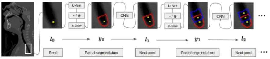
RavelNet relies on two trained machine learning models: a RNN and a U-Net. Once both have been trained, the segmentation process works as illus-trated in Fig.4. First, an initial seed on the anatomy centerline is dened. Currently, the seed is obtained via clinician placed landmark points but future work will automate this initialization. Next, our U-Net predicts a partial segmentation of the anatomy near the seed. This predicted segmen-tation is then used by the RNN to predict the next centerline point and the process continues forT iterations. After termination, the full segmentation is reconstructed from the partial ones. In the following sections, we describe this process more formally.
Fig. 4. The locationl0is used the predict the segmentation y0(U-Net +
region growing) which is then used to predict the next location (RNN).
3.2.1 Task
Given an input imageI, we seek a binary segmentationywhere anatomy
voxels are assigned a 1 and all other voxels are assigned a 0. We break the task into two steps: centerline prediction and patch segmentation. Each step is handled using an independently trained deep model.
3.2.2 Centerline Prediction
The goal of this sub-task is to learn to predict tubular anatomy center-lines from their segmentations.
Each location vector lt has a corresponding segmentation patch yt obtained by rst, rotating the segmentation y about the centerline point
such that the cross sectional normal is parallel to thezaxis and by second,
cropping a 166464 patch centered at the same point from the rotated segmentation. This patch needs to be large enough to hold the anatomy and may be adjusted depending on the image size.
Hence, given a segmentation and a point on the centerline, the infer-ence task is the compute p(ltjy0;l0). We assume that the location vectors
fltgfollow a rst order Markov chain. That is:
p(ltjy0; ::::; yt¡1;l0; ::::; lt¡1) =p(ltjyt¡1; lt¡1) (1)
Learning: We learn a representation of p(ltjyt¡1;lt¡1) using an RNN given a training dataset of centerline location vectors and corresponding seg-mentation patches. Centerlines are extracted from the segseg-mentations [7] and location vectors are sampled uniformly from them. Specically, we consider a training dataset of N segmentations fyigiN=1¡1, each of which has a
cor-responding sequence of location vectorsl0i; ::::lTi and segmentation patches
y0i; ::::;yTi. The paramter value to be learned by the RNN islcorresponding to p(ltjyt¡1; lt¡1;l). In practice, we split the location vector into its location partltlo cand its orientation partltoriand seek the parameter value that minimizes the mean squared error of the location and the angle-in-between of the orientation. Hence, our loss function is
L(l) =
X
t=1 T
ltlo c 0
¡ltlo c 2
+arccos ltori 0
ltori
kltori 0
k kltorik
!
(2)
where ltlo c 0
and ltori 0
come from the model prediction given yt¡1; lt¡1; l. Note that maximizing the likelihood of observed sequences in this way is known as teacher forcing and has the added benet of decoupled time steps.. That is, the output at each time step only depends on the previous time step's output.
Inference: Under the rst order Markov chain asusmption (1), we can write our inference task as:
p(ltjy0;l0) =
X
t¡1
p(ltjyt¡1; lt¡1)p(ltjy0;l0) (3)
Computing this using recursion is intractable because the summation goes over all possilbe centerlines and corresponding segmentation patches. We follow the widely accepted practice of using the most likely location vector
lt¡1and corresponding segmentation patchyt¡1as input to the subsequent computation:
RNN: We implement our centerline prediction model as a RNN which is formed by connecting copies of identical CNNs (Fig.3) trained to estimate
lt given yt¡1 and lt¡1. Thus, paramteres are shared both spatially and temporally. TThe CNN is simply 2 layers of 333 convolutions and ReLU followed by 2 fully connected layers with 512 and 6 units respectively. In practice, we combineyt¡1andlt¡1by setting the voxel containing the cen-terline location equal to¡1, thereby cuing the RNN as to where the origin for calculating the location displacement to the next centerline point should be.. At each time step, our CNN inputs the most likely segentation from the previous stepaugmented as describedto predict the next location vector. This respects the Markov property as there are no connections between successive RNN steps.
3.2.3 Patch Segmentation
The goal of this sub-task is to predict partial segmentations given a location and orientation on the anatomy centerline.
U-Net: We use the original U-Net as a rst pass for segmentation. Along with a segmentation patch, each location vector also has a corre-sponding image patchItextracted fromIin the same way the segmentation patch is extracted. We consider a training dataset of N T image patches
fIigi=0
NT¡1 and corresponding segmentation patches fy igi=0
NT¡1 extracted
fromN images and segmentations atT centerline points. We train to
mini-mize the binary cross-entropy between the prediction and the ground truth. Hence, our losss function is
L¡Y ; Y0=¡ 1
N T X
b=1 NT
1
2YblogYb 0
(6)
whereY andY0denote the attened prediction and ground truth
segmen-tations of thebthimage.
We are concerned with predicting segmentation bounds. Thus, we take the logical complement of the segmentation and dilate it to getbi=A(:
yi)where Ais the cube structuring element of size 555.
Region Growing: We use region growing as a second pass. Starting at the centerline point, we grow our region infIigto its 6 connected voxels with the criteria that each new voxel intensity must be withinaof the mean
region intensity. We do not grow to voxels that are inbiand we determine
aand by randomly sampling 100 values for each and selecting the values
that maximize the average Dice coecient of segmentations obtained from
fIigonfyig.
Once the U-Net and RNN are trained, the segmentation is completely automatic given the initial seed. At each time step of the RNN, we extract an image patchIt¡1from our imageI usinglt¡1 and get its segmentation
yt¡1. Our RNN then uses the location augmentedyt¡1to predictlt. After
T iterations, we have overlaping segmentation patches for every point along
the centerline and the full segmentation y can be reconstructed (Fig.4).
Patch overlap is ensured by sampling centerline points suciently close to each other while keeping in mind the patch size.
4 Experiments
4.1 Synthetic Data
We use two dierent sets of synthetic data: one designed to mimic the airway and another designed to mimic the colon. Both are of size 128128128. We rst dene a canonical centerline for each by hand. Specically, we dene landmark points for the centerline and subsequently spline interpolate a smooth curve through uniformly perturbed versions of the landmark points for each sample. We then generate the anatomy by connecting circles of varying radii at each centerline point.
The circle radii for the airway increase from the trachea (Uniform(6, 8)) to the nose tip (Uniform(9, 18)) while they stay the same throughout for the colon (Uniform(6, 15)). We augment the data by rotating the volumes along each axis randomly between [0, 300]. To generate the medical image, we create a volume where each voxel is Uniform(0,1). We then set voxels corresponding to the anatomy equal to 0 and apply a Gaussian blur withs= 3. Additionally, for the airway, we also add noise in the form of Uniform(2, 5) spheres of radius 5 uniformly placed within 20 voxels of the nose tip to model the sinuses. We generate 50 of each synthetic anatomy and use 40 for training and 10 for testing (Fig.5).
4.2 Clinical Data
We use pediatric airway CT scans of size (512¡591)(512¡582)(162¡1021) and resolution (0.25¡0.74)(0.25¡0.74)(0.3¡0.9)mm3per voxel for evalu-ation. We normalize the intensities of each image such that the 0.1 percentile and the 99.9 percentile are mapped to {0, 1} and clamp values that are smaller and larger to 0 and 1 respectively. We have 30 CTs and corre-sponding human-guided segmentations. Human-guided in this case means that the segmentations were obtained by carrying out manual operations such as clipping undesired parts and correcting under-segmented bits but are not necessarily fully hand annotated. We use 25 for training and 5 for testing. Centerlines are inferred from the airway segmentations based on the heat distribution along the airway ow as solved by a Laplace equation [7].
4.3 Competing Methods
We compare four dierent methods of tubular anatomy segmentation. DIR-UNET uses the original U-Net to predict segmentations directly from down-sampled versions of the medical image. We down-sample to 12812864 because 3D convolutions have high memory demands and full sized images do not t on our GPU. PATCH-UNET predicts segmentations using over-lapping tiles of size 12812864 as in the original U-Net [2]. Patches are sampled so that each voxel (except those near the border) is covered by 8 patches. Reconstruction simply takes the average of the 8 predictions for the voxel. RAVELNET-R is our method as described above. And nally, RAVELNET-NR is our method as described above but without the region growing step. That is, we use the output of the U-Net directly to reconstruct and to predict the next centerline point.
4.4 Evaluation
We evaluate each method using three metrics: 1) Dice coecient to mea-sure the accuracy of the nal segmentation, 2) memory consumption during training, and 3) number of connected components in the segmentation (ide-ally this should be 1). We also run each trial using 100% of the training data and 50% of the training data (50% to simulate a scenario with limited segmentation annotations).
5 Results
5.1 Overview
The evaluation results on the synthetic and pediatric airway test sets are shown in Tab.1. RAVELNET-R outperformed PATCH-UNET on all trials by an average Dice coecient margin of 3.75. Most notably, RAVELNET-R outperformed all other tested approaches on the airway dataset when using 100% of the training data. This strongly supports our hypothesis that unraveling the anatomy along the centerline simplies the segmentation task by bringing it into a more natural image space (Fig.6).
While both RAVELNET approaches demonstrated similar overall average Dice scores, RAVELNET-R outperformed RAVELNET-NR on the airway dataset by an average Dice coecient margin of 0.5. Furthermore, RAV-ELNET-R demonstrated the lowest average number of connected components at 1, indicating that it has eectively eliminated the need for post-pro-cessing to ensure connectivity.
Fig. 6. Synthetic airway getting unraveled by the RNN to make the seg-mentation task simpler. The left image shows the original volume. The top image shows the unraveled volume along the centerline. The bottom image shows the segmentation.
5.2 Memory Usage
RAVELNET approaches use 326464 patchs centered at centerline points to train U-Net whereas both UNET approaches use 12812864 patches. RAVELNET includes an additional CNN but the memory costs of 2 layers of 333 convolutions and 2 fully connected layers are negligible in com-parison to the U-Nets. Hence, the UNET approaches have approximately 8 times as many model parameters as RAVELNET and thus, consume approx-imately 8 times as much memory during training.
5.3 Traininig Data Size
os are similar, RAVELNET approaches outperformed UNET approaches when 50% of the training data was used by an average Dice coecient margin of 8. Note that both RAVELNET approaches using 50% of the training data still outperformed the DIR-UNET approaches using 100% of the training data in all conducted trials.
DIR-UNET PATCH-UNET RAVELNET-R RAVELNET-NR S-Col 1 Dice: 75Comps: 1.53 Dice: 88Comps: 1.85 Dice:Comps:901 Dice:Comps:901
S-Col 5 Dice: 71Comps: 1.68 Dice: 82Comps: 2.03 Dice:Comps:881 Dice:Comps: 1.0488
S-Air 1 Dice: 84Comps: 1.88 Dice: 89Comps: 2.03 Dice: 92Comps:1 Dice:Comps: 1.1193
S-Air 5 Dice: 82Comps: 2.29 Dice: 87Comps: 2.32 Dice:Comps:911 Dice:Comps: 1.1291
Air 1 Dice: 71Comps: 9.44 Dice: 81Comps: 13.19 Dice:Comps:881 Dice: 86Comps: 2.33
Air 5 Dice: 59Comps: 8.39 Dice: 69Comps: 16.32 Dice: 72Comps:1 Dice:Comps: 4.0173
Table 1.Dice and connected components evaluation of DIR-UNET, PATCH-UNET, RAVELNET-R and RAVELNET-NR methods on synthetic and airway test datasets. Both Dice and number of connected components are averaged over all test samples.
6 Conclusion
We presented RavelNet, a novel scheme for segmenting tubular structures that is sensitive to anatomy curvature and connectivity. Not only did Rav-elNet outperform state-of-the-art segmentation methods on synthetic tubular structures and pediatric airways, it did so using less training data, less memory and while maintaining segmentation connectivity. Our work demon-strates that unraveling tubular structures along their centerlines simplies the segmentation task by bringing the task into a more natural domain. Future work will investigative training RavelNet end-to-end.
7 References
1. Mohan V., Sundaramoorthi G.: Tubular Surface Segmentation for Extracting Anatomical Structures From Medical Imagery. TMI, vol. 12 (2010)
3. Goodfellow, I., Bengio, Y., Courville, A.: Deep Learning. MIT Press, Cambridge (2016)
4. Cohen L., Descamps T.: Segmentation of 3D tubular objects with adaptive front propagation and minimal tree extraction for 3D medical imaging, Comput Methods Biomech Biomed Engin, vol. 10 (2007)
5. Behrens T., Rohr K., Stiehl S.: Robust Segmentation of Tubular Struc-tures in 3-D Medical Images by Parametric Object Detection and Tracking, IEEE Trans Syst Man Cybern, Part B (2003)
6. Bruijne M., Ginneken B., Viergever M., Niessen W.: Adapting Active Shape Models for 3D Segmentation of Tubular Structures in Medical Images, Information Processing in Medical Imaging (2003)
7. Hong Y., Niethammer. M, Johan A., Kimbell J., Pitkin E., Superne R., Davis S., Zdanski C., Davis B.: A Pediatric Airway Atlas and its Appli-cation to Subglottic Stenosis, ISBI (2013)
8. Pace D., Dalca V., Brosch T., Geva T., Powell A., Weese J., Moghari M.: Iterative Segmentation from Limited Training Data: Applications to Congenital Heart Disease, DLMIA 2018 (2018)
9. Li. K, Hariharan B., Malik J.: Iterative Instance Segmentation, CVPR (2016)
10. Roychowdhury S., Koozekanani D., Parhi K.: Iterative Vessel Seg-mentation of Fundus Images, IEEE Trans Biomed Eng, vol. 62 (2015)
11. Stoyanov D., Taylor Z.: Deep Learning in Medical Image Analysis and Multimodal Learning for Clinical Decision Support, Springer Nature (2018)
12. Schlemper J., Caballero J., Hajnal J., Price A., Rueckert D.: A Deep Cascade of Convolutional Neural Networks for Dynamic MR Image Recon-struction, IEEE Transactions on Medical Imaging (2018)
13. Norouzi A., Saba T., Ehsani A.: Medical Image Segmentation Methods, Algorithms, and Applications, IETE Technical Review (2014)
14. Krizhevsky A., Sutskever I. Hinton G.: ImageNet Classication with Deep Convolutional Neural Networks, Advances in Neural Information Pro-cessing Systems (2012)
15. Ciresan D., Giusti A., Gambardella L., Schmidhuber J.: Deep Neural Netoworks Segment Neuronal Membranes in Electron Microscopy Images (2014)
16. Yu F., Koltun V.: Multi-Scale Context Aggregation by Dilated Con-volutions, ICLR (2016)