Abstract. The focus of this thesis is on estimation of the in-degree distribution in directed networks from sampling network nodes or edges. A number of sampling schemes are con-sidered, including random sampling with and without replacement, and several approaches based on random walks with possible jumps. When sampling nodes, it is assumed that only the out-edges of that node are visible, that is, the in-degree of that node is not observed. The suggested estimation of the in-degree distribution is based on two approaches. The inversion approach exploits the relation between the original and sample in-degree distributions, and can estimate the bulk of the in-degree distribution, but not the tail of the distribution. The tail of the in-degree distribution is estimated through an asymptotic approach, which itself has two versions: one assuming a power-law tail and the other for a tail of general form. The two estimation approaches are examined on synthetic and real networks, with good performance results, especially striking for the asymptotic approach.
1. Introduction
Driven by the explosion of data on a host of real world networks, the last few years have seen vigorous activity from a number of communities including computer science, statistical physics and the social sciences to develop methodology to explore large scale networks as well as formulate network models to understand the emergence of various properties of real world systems such as the high degree of clustering, heavy tailed degree distribution and so on Albert and Barab´asi (2002); Newman (2018).
One particular corner of this vast field of great importance is the setting of directed net-works. Real world examples include:
(i) Information and social networks: Canonical examples of these objects include the internet at the webpage level with a directed edge from page A toB if webpage
A has a link toB Broder et al. (2000); Brin and Page (1998) or Twitter networks at various levels including edges from person A to B if person A follows B or Twitter event networks over a fixed duration where one follows particular hashtags and there is an edge fromAtoB ifAretweetsB in the time interval of interest Beguerisse-D´ıaz et al. (2014); Golder and Yardi (2010). One need not overstate the impact of the above networks both for every day activities as well as in determining politics and world events such as the Arab Spring Khondker (2011).
(iii) Citation networks: Here the data object consists of papers in a single discipline such as condensed matter physics or across multiple disciplines Redner (2004); Vazquez (2001). While the data can be parsed as both directed or undirected networks at various resolutions, one canonical object of interest is via a directed network where we put an edge from paperAtoB if paperAcitesB. Analysis range from exploration and clustering into sub-communities (see Barab´asi et al. (2002); Newman (2004) and the references therein) to detecting emerging areas or understanding the evolution of these networks over time.
(iv) Trophic networks in ecology: Here one is interested in feeding relationships amongst species with directed edge from A to B if species A preys on B (in many cases vertex sets can be more general than species ranging from “taxonomically related groups of species to whole kingdoms . . . or even non-living organic matter” Pascual and Dunne (2005)). Questions of interest include estimation of such food webs from data, stability of the resulting systems to invasion of new species or fluctuations in density of existing species, robustness including the number of secondary extinctions triggered by loss of primary species as well as classification of keystone species.
For many real directed networks, the in-degrees (i.e. the number of in-edges) of nodes and their distribution are of particular interest. To fix ideas, consider, for example, the Amazon product co-purchasing network Leskovec et al. (2007), where a directed edge from product
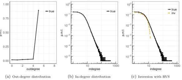
A to product B indicates that after buying A, a customer also would often purchase B,1 after the latter appears in the Amazon recommendation feature “Customers Who Bought This Item Also Bought This.” The number of recommended products B to purchase along with A is generally small. As a result, the out-degree of a node (product) A is limited (in the considered dataset, it is limited by 5), and the out-degree distribution is not particularly interesting, as depicted in Figure 1(a). For this network, the in-degrees and their distribution are of greater interest. For example, the nodes with high in-degrees are the products B that are also purchased when buying other products. The range and the shape of the in-degree distribution could also be of interest. The in-degree distribution for the Amazon product co-purchasing network is depicted in Figure 1(b), on the log-log scale, and the straight tail suggests, in particular, that the distribution has a power-law tail. Similar observations apply to many other directed networks, for example, citation networks that will also be considered for illustration in this thesis, or web link networks.
Furthermore, many real directed networks are extremely large, with large numbers of nodes and edges. Even the Amazon product co-purchasing network discussed above, which can be considered on the “smaller” side, already has 262,111 nodes and 1,234,877 edges. The Internet at the webpage level is estimated to have over 1.5 billion nodes (webpages). For such networks, it may be prohibitively expensive to gather all the information necessary to produce the in-degree distribution. To overcome this issue, sampling of nodes or edges seems to be a natural approach where the quantity of interest (the in-degree distribution in our case) would have to be inferred from the sampled data. Not surprisingly, sampling has been used extensively to deal with large networks and to infer their various quantities of interest but the in-degree distribution has received less attention yet. Some related references are discussed below, after we first describe our methods in some detail.
1There seems to be some confusion in the literature on whether to callBco-purchased withA, or the other
0.00 0.25 0.50 0.75 1.00
0 2 4 6 8
outdegree
p
.m.f
.
true
(a)Out-degree distribution
10−5 10−4
10−3 10−2 10−1 100
10 1000
indegree
p
.m.f
.
true
(b)In-degree distribution
10−5 10−4 10−3 10−2 10−1 100
10 1000
indegree
p
.m.f
.
true inv
(c)Inversion with RVS
Figure 1. Amazon product co-purchasing network.
We are thus interested in inference of the in-degree distribution through sampling network nodes and edges. Several key issues arise that we shall discuss briefly, with the goal of indicating our contributions as well:
• Inherent difficulty of the problem: the latent nature of node in-degrees.
• Sampling schemes to use: novel schemes based on random walks.
• Inference approaches from statistical standpoint: application of penalized inversion approach and a new asymptotic approach.
An inherent difficulty in inferring the in-degree distribution is that, for example, when sam-pling a node, its in-degree is not observed but rather only its out-edges are seen, which contribute to the sample in-degrees of its neighbors. For example, this is very different from inferring the out-degree (or just the degree for undirected networks) distribution since the true out-degree of a sampled node is observed.
the extensive use of random walks to sample networks can be found below. We should also note that though related, the PageRank distribution is not the in-degree distribution.
Inference approaches: application of penalized inversion approach. Turning to statistical inference, the problem of inference for the in-degree distribution from sampled data is that of statistical inversion. More specifically, ifd= (d(j), j = 0, . . . , J), is the in-degree distribution of a network andds = (ds(j0), j0 = 0, . . . , J0) is its sample counterpart, we first
show that
ds =Psd
for a specified matrixPs which depends on the chosen sampling scheme. Part of our
contri-butions is deriving the analytical expressions forPs under the considered sampling schemes.
An inversion estimator ofdis defined as db=Ps+dbs, wherePs+ is a suitable inverse of Ps and
b
ds refers to the distribution of sample in-degrees. A penalized version of this “naive”
esti-mator will also be considered, following the work of Zhang et al. (2015), in order to improve on its performance. The performance of this penalized estimator for the Amazon product co-purchasing network is illustrated in Figure 1(c), when using RVS with the node sampling probability of 15%.
Inference approaches: a new asymptotic approach. As can be seen from the latter figure, the inversion approach does not work well in the tail of the in-degree distribution due to the inherent difficulty of the problem described above. To address estimation in the tail, we also study an asymptotic approach, assuming either an arbitrary or power-law tail of the in-degree distribution. This approach essentially involves a suitable rescaling of the sample in-degree distribution. See, for example, Figures 2–4 for illustration. The asymptotic approach for the Amazon product co-purchasing network is depicted in Figure 5. The inver-sion and asymptotic approaches, when combined together, can estimate the whole in-degree distribution.
Concerning related work, sampling-based estimation of degree distribution in undirected networkswas considered by many researchers, for example, Stumpf and Wiuf (2005), Leskovec and Faloutsos (2006), Ribeiro and Towsley (2010, 2012), Gjoka et al. (2011), Kurant et al. (2011), Lee et al. (2012), Zhang et al. (2015), to name but a few. Various sampling schemes and associated inference approaches for this task were considered, most often based on dif-ferent forms of random walks. Other characteristics studied under sampling in undirected networks include global clustering coefficient (e.g. Ribeiro and Towsley (2010)), network size (e.g. Katzir et al. (2011)), number of triangles (e.g. Wu et al. (2016)), and others.
Turning todirected networks, Henzinger et al. (2000) and Bar-Yossef and Gurevich (2008) add reversed links when sampling a directed network through random walks to avoid being “trapped” and in this way, build over it an undirected network, which is then used to sample nodes at random. Ribeiro et al. (2012) also follow this idea by introducing a Directed Unbiased Random Walk (DURW), which combines the usual random walk on a directed network with occasional jumps. See also Murai et al. (2017). One of the random walks considered in this work is similar to DURW. Sampling algorithms in directed networks based on PageRank are studied in Leskovec and Faloutsos (2006), Salehi and Rabiee (2013). Out-degree distribution was among network characteristics studied under some of these sampling schemes. But as noted above, inference of the in-degree distribution has seemingly not been addressed yet (though discussed in e.g. Ribeiro et al. (2012)).
the in-degree distribution through statistical inversion is studied in Section 3. The section is divided into a number of parts based on the sampling scheme used. The asymptotic approach is described in Section 4. The proposed estimation methods are examined on synthetic and real networks in Section 5. Conclusions can be found in Section 6.
2. Sampling framework and sampling schemes
2.1. Directed graphs. Let Gd = (V, Ed) be a (simple) directed graph representing the
network of interest with Nv = |V| number of vertices (nodes) and Ne = |Ed| number of
directed edges. We denote a generic vertex as v, v0 or u or, if more than one vertex is considered, as vi, etc. Similarly, the notation for edges is e, e0, ei, etc. The subscripts “v”
and “e”, on the other hand, will indicate that the corresponding quantities (e.g.Nv and Ne)
are associated with vertices and edges, respectively. A directed edge from a vertex u to a vertex v will be denoted by (u, v), that is, (u, v)∈Ed. We shall also denote a directed edge
as (u → v), to contrast it with edges in undirected graphs that will also be considered in some instances below. We assume that each vertex in Gdhas at least one (either in- or out-)
edge. For notational simplicity, we shall also sometimes write v ∈ Gd (rather than v ∈ V)
and e∈Gd (rather thane∈Ed).
2.2. In-degree and other quantities of interest. We focus throughout this work on the in-degree of a vertex v, that is,
X(v) :=|{u: (u, v)∈Ed}|=
Nv
X
k=1
1{(uk,v)∈Ed} (1)
and the in-degree distribution of the graph Gd, that is,
d(j) := PJD(j)
j=0D(j)
:= |{v:X(v) =j}|
Nv
=
PNv
k=11{X(vk)=j} Nv
, j= 0,1, . . . , J, (2)
where D(j) is the number of vertices having in-degree j, referred to as an in-degree count, and J(≤Nv −1) is the maximal in-degree in Gd. Note that D(0) is non-zero if Gd contains
vertices with out-edges but no in-edges.
We are interested in estimating the in-degree distribution (2) through sampling. This is also equivalent to estimating the in-degree counts D(j). We will sample either vertices or edges, which we shall refer to as sampling objects. When sampling a vertex, we assume importantly that onlyout-edges and out-neighbors of the vertex are “visible.” This is a common scenario encountered with real networks. The corresponding out-edges make the sampling information retained for that sampled vertex. When sampling an edge, we assume the edge to be directed and to be the sampling information retained for that sampled edge. We shall denote the (possibly repeated) sampled objects as si, i = 1, . . . , n, further writing si = vi, n = nv for
vertices and si=ei,n=ne for edges. The various sampling schemes considered in this work
are discussed in Section 2.3.
For a collected sample of size n, let
b Xs(v) =
n
X
i=1
wheresi,i= 1, . . . , n, refer to the sampled objects (i.e. vertices or edges), and
b Ds(j0) =
Nv
X
k=1
1{ b
Xs(vk)=j0}, j
0 = 0,1, . . . , J0. (4)
The quantitiesXbs(v) and Dbs(j0) are the sample analogues of X(v) in (1) and D(j0) in (2),
respectively, as suggested by the subscript “s”. Note that J0 in (4) need not be the same as
J and could even be larger as in sampling with replacement (discussed in this section below). The quantitiesDbs(j0)’s will be modified in Sections 3 and 4 below to yield suitable estimators
b
D(j)’s ofD(j)’s.
It will also be convenient to think about X(v) in (1) and Xbs(v) in (3) for a typical vertex v, namely, a vertex chosen (uniformly) at random. Thus, we also let X=X(v∗) denote the in-degree of a vertexv∗ chosen at random. Note that
P(X =j) =d(j). (5)
Additionally, letXs =Xbs(v∗) be the sample in-degree of a vertexv∗ chosen at random from
the graph after sampling. We also set
ds(j0) :=P(Xs =j0), Ds(j0) =Nvds(j0). (6)
Note that
EDbs(j0)
Nv
=E1{Xbs(v∗)=j0} =P(Xs=j 0
) =ds(j0) =
Ds(j0)
Nv
. (7)
Note also that we do not put a hat on Xs and that Ds(j0) involves normalization by Nv
(rather than, for example, by the average number of sampled vertices).
2.3. Sampling methods. We consider several sampling schemes. At the highest level, we shall distinguish between sampling with replacement (WR) and sampling without replacement (NR), the latter an acronym for “No Replacement.” In sampling without replacement, only distinct sampled objects (vertices or edges) are included in the retained information. In sampling with replacement, the same sampled objects (vertices or edges) can be included in the retained information. Samplings with and without replacement are expected to be different only when the number of sampled vertices (edges) is relatively large compared to the total number of vertices (edges). This is often the case in the setting of sampling networks where the percentage of sampled vertices (edges) have ranged in 10%-30% of the total population Zhang et al. (2015).
2.4. Random walk samplings. We introduce below three random walk sampling (RWS) schemes: RWS1, RWS2 and RWS3. In a “stationary” regime, RWS1 will correspond to RVS-WR, and RWS2 and RWS3 to RES-WR. Before presenting their constructions and to facilitate the reading, we should also indicate several of their aspects that should not be surprising. Note that without any modification, a random walk on a directed graph might be “trapped” at a vertex without out-edges. This is often rectified by allowing the random walk to “backtrack,” that is, to walk on the directed edge backwards, thus essentially making it undirected Bar-Yossef and Gurevich (2008). With our RWS schemes, we shall thus be building undirected graphs on top of the directed graph as the walk progresses. In addition, it is also common to introduce the possibility of jumps with RWS Murai et al. (2017). We shall allow for jumps as well and their exact role will be discussed further below. In particular, the key difference between RWS2 and RWS3 is that the walk jumps to edges in RWS2 and to vertices in RWS3.
RWS1. We construct here a RW on a suitable graph whose stationary distribution is uniform over the graph vertices, and thus corresponds to RVS-WR. Then, a sample of vertices can be selected by using such a RW and the estimation methods for RVS discussed in Sections 3 and 4 can be applied.
In addition to the directed graph Gd, our random walk constructs and uses an undirected
multigraph constructed from Gd, which we denote by Gi at step i. The walk will also make
occasional jumps to vertices chosen at random in the graphGd, the probability (rate) of which
will be associated with a parameter w ≥ 0. The case w = 0 corresponds to no jumps, and
w=∞ to jumps only. The construction of the walk is summarized in the pseudo Algorithm 1. The set S gathers the sampled, possibly repeated vertices and R the previously visited vertices. In Step (1), the undirected graphGi−1 is augmented toGiby including all out-edges from a vertexv added to the sampleS. Step (2) selects a candidate vertex u, which in Step (3) is either selected as the next vertex v to be added in the sample or the same vertex v
is repeated in the sample. After the algorithm is run, the information kept consists of the out-edges seen from the vertices collected inS.
A number of further comments are in place regarding Algorithm 1. We think of Gi as
an undirected multigraph which asi increases, becomes the undirected multigraphG∞ con-structed from Gd by making all directed edges undirected. The selection of u in Step (2)
corresponds to the transition probabilities
Pi(v, u) =
1{(v,u)∈Gi} w+ degi(v) +
w w+ degi(v)
1
Nv
, (8)
when selecting u for a given v. The stationary distribution of these transition probabilities (in the limit of large i) is not uniform on the vertices. But it could be made uniform in a standard way through a Metropolis-Hastings (MH) algorithm as in Step (3) by noting that
w+ degi(v)/w+ degi(u) appearing in that step is the MH acceptance function. Indeed, this follows by noting that
Pi(u, v)
Pi(v, u)
=
1{(u,v)∈Gi} w+ degi(u) +
w w+ degi(u)
1
Nv
. 1{(v,u)∈Gi} w+ degi(v) +
w w+ degi(v)
1
Nv
= w+ degi(v)
Algorithm 1: RWS1
Initialization: Choose a vertexv at random from Gd. Setw,nv,i= 1,G0 =∅ and
S={v} (for the sample),R=∅ (for the previously visited vertices).
Loop: Whilei < nv:
(1) Gi=Gi−1∪ {(v, v0) : (v →v0)∈Gd, v /∈R}.
(2) GenerateU1 uniformly on (0,1) and let degi(v) be the degree of the vertex v inGi. IfU1 <degi(v)/(w+ degi(v)), choose the potential next vertex u at random from
the neighbors of vin Gi. Otherwise, chooseu at random from the vertices of G d.
(3) GenerateU2 uniformly on (0,1). If U2 <(w+ degi(v))/(w+ degi(u)), updatev asu. Otherwise, repeatv as the next vertex. (If u /∈Gi, degi(u) should be read as zero.) (4) R←S,S←S∪ {u}.
(5) i←i+ 1.
Output: S (the sample of size nv).
As noted above, this argument should be viewed withi=∞ on G∞, that is, in the limit of largei.
We also note that a burn-in period could be added in Algorithm 1 where the sample starts being collected only after a certain number of stepsiin the algorithm have been completed. The proposed random walk, without the MH correction, is also related to the DURW studied by Ribeiro et al. (2012).
Remark 2.1. There are several reasons why jumps are used in RWS1. By varying w (from
w= 0 corresponding to no jumps tow=∞ associated with jumps only), their effect can be assessed on the performance of the estimation methods. For example, our inversion methods are quite insensitive to the proportion of jumps but the asymptotic approaches require a fairly large proportion of jumps. A related question is why not use only jumps or, equivalently, RVS, if such sampling is possible. From a practical perspective, RWs without any jumps would be preferred over RVS, since this is how real networks are typically explored. RWS schemes are thus viewed as primary approaches, which are supplemented by jumps to improve performance if needed. Another potential advantage of RWs with jumps over RVS is that jumps could be imposed only to an available subset of the graph vertices or even only to vertices from the undirected graph built from the RW.
We turn next to RWs where in a “stationary” regime, edges will be sampled at random and hence the estimation based on RES-WR can be used. We consider two RW versions, RWS2 and RWS3 below, depending on whether a jump in RW chooses an edge or a vertex at random, respectively.
RWS2. A pseudo algorithm for this sampling scheme is given in Algorithm 2. We again think of Gi as an undirected multigraph which as i increases, becomes G∞, the undirected multigraph constructed from Gd by making all directed edges undirected. Several further
Algorithm 2: RWS2
Initialization: Choose an edge (v1→v2) at random from Gd. Setw,ne,i= 1,G0 =∅,
S={(v1 →v2)}(for the sample), R=∅ (for the previously visited vertices) and jump= 1.
Loop: Whilei < ne:
(1) Gi=Gi−1∪ {(v1, v) : (v1→v)∈Gd, v1 ∈/ R} ∪ {(v2, v) : (v2 →v)∈Gd, v2 ∈/ R}.
Edges are added as undirected but their directionality inGd is kept as an attribute.
Also update R←R∪ {v1, v2}.
(2) Ifjump= 1, choose v asv1 orv2 at random and setjump= 0. Otherwise, set
v=v2.
(3) GenerateU uniformly on (0,1). IfU <1/(1 +w), set (v1 →v2) as an edge selected at random from {(v, u)∈Gi}with directionality determined by the attribute inGi. Otherwise, update (v1 →v2) as an edge selected at random fromGd, and set
jump= 1.
(4) S←S∪ {(v1 →v2)}.
(5) i←i+ 1.
Output: S (the sample of size ne).
undirected but they are also attributed the edge direction fromGd. We need to keep track of
the direction in the collected sample since we are interested in the in-degree distribution and use the RES estimation that employs directional edges. In Step (1), the undirected graph
Gi−1 is augmented to Gi by adding all out-edges from the two vertices v1 and v2 of the directed edge (v1 →v2) added to the sample. In Step (2), if the vertex (v1 →v2) was jumped
to (thus jump= 1), one of its vertices v1 orv2 is chosen at random as v through which the RW will further explore the graph. On the other hand, if the vertex (v1 → v2) was chosen through a non-jump step of the RW (jump= 0), this means that the RW previously visited the edge where v2, was one of the vertices – in this case, the RW will further explore the graph through the vertexv=v2.
The motivation for selecting a new directed edge into the sample in Steps (3) and (4) is as follows. For largei, we can think of Gi as the undirected multigraph G∞, defined from Gd
as above. The graphsG∞ and Gd have the same edges, except that in Gd, these are made
directional. The key observation then is that our algorithm samples edges at random from
G∞, and hence once attributes are added, also directed edges at random fromGd. Indeed, to
prove this key observation, it is enough to show that the stationary distribution of our RW on edges is uniform. For this, note that according to our algorithm, the transition probability for the RW on G∞ is
P((v1, v2),(u1, u2)) =
1 X
k=0
P((v1, v2) to (u1, u2)|jump=k)P(jump=k)
=P0((v1, v2),(u1, u2))
1
1 +w +P1((v1, v2),(u1, u2)) w
1 +w, (10)
with
P0((v1, v2),(u1, u2)) =
1{(u1,u2)∈N∞(v2)}
deg∞(v2)
1 1 +w+
2 vol(G∞)
w
and
P1((v1, v2),(u1, u2)) = 1 2
2 X
j=1
1{(u1,u2)∈N∞(vj)}
deg∞(vj)
1 1 +w+
2 vol(G∞)
w
1 +w !
,
where deg∞(v) stands for the degree ofvinG∞,N∞(v) refers to the neighborhood ofvinG∞
(that is, the edges connected tov), and vol(G∞) =P
v∈G∞deg∞(v) is also twice the number
of edges in the multigraphG∞. With some abuse of the notation and to keep notation simple, if there are two edges inG∞ between two vertices u1 and u2, we denote both of these edges
as (u1, u2). The uniform distribution π((v1, v2)) = 2/vol(G∞) on the edges is the stationary distribution for the RW sinceP
(v1,v2)P((v1, v2),(u1, u2)) = 1 (i.e. P is a doubly stochastic
transition matrix). This follows fromP
(v1,v2)Pk((v1, v2),(u1, u2)) = 1 for k= 0,1 since, for
example, fork= 1,
X
(v1,v2)
P1((v1, v2),(u1, u2)) = X
(v1,v2)
1 2
2 X
j=1
1{(u1,u2)∈N∞(vj)}
deg∞(vj)
1 1 +w +
2 vol(G∞)
w
1 +w !
= X
(v1,v2)=(u1,u2)
1 2 2 X j=1 1 deg∞(vj)
+ X
v1=u1,(v1,v2)6=(u1,u2)
1 2deg∞(v1)
+ X
v2=u2,(v1,v2)6=(u1,u2)
1 2deg∞(v2)
!
1 1 +w+
w
1 +w
= 1 2 2 X j=1 1 deg∞(uj)
+deg∞(u1)−1 2deg∞(u1)
+deg∞(u2)−1 2deg∞(u2)
!
1 1 +w +
w
1 +w
= 1
1 +w + w
1 +w = 1. (11)
RWS3. We finally turn to a random walk for sampling edges where jumps will be to ran-dom vertices rather than edges. Jumping to ranran-dom vertices might be preferred within the architecture of many real networks. A pseudo algorithm for RWS3 is included as Algorithm 3, and we comment on its steps and motivation next.
As in RWS2, for largei, we think ofGias the undirected multigraphG∞constructed from
Gd by making its directed edges undirected. Let also deg∞(v) be the degree of a vertexv in G∞. When Algorithm 3 acts onG∞, we shall argue that it selects the edges ofG∞at random (and hence also the edges of Gd at random, with the directionality kept as an attribute in
Algorithm 3). To make such an argument, we add an “imaginary” vertexgtoG∞and connect it to each vertex ofG∞through an edge that carries a weightw≥0. Other edges in G∞ are then assumed to have weight 1. The resulting multigraph with the added “imaginary” vertex and edges is denotedGe∞. The edge weight,wor 1, plays a role only when sampling randomly
from a collection of edges, in which case their weights determine the sampling probabilities. For example, two edges with weights 1 and w = 2 would be sampled with the respective probabilities 1/(1 +w) = 1/3 andw/(1 +w) = 2/3.
Now, note that Step (3) of Algorithm 3 can be reformulated forGe∞by stating that an edge
is selected randomly from{(v, u)∈Ge∞}, with the edge weights determining sampling
Algorithm 3: RWS3
Initialization: Choose a vertexv at random from Gd. Setw,ne,i= 1, G0 =∅,S=∅
(for the sample) andR=∅ (for the vertices visited by RW).
Loop: While|S|< ne:
(1) Gi=Gi−1∪ {(v, u) :v /∈R, (v→u)∈Gd}. Edges are added as undirected but their
directionality inGd is kept as an attribute.
(2) R←R∪ {v}.
(3) GenerateU uniformly on (0,1) and let degi(v) be the degree of the vertexv inGi. If
U <degi(v)/(degi(v) +w), choose an edge (v1→v2) at random from {(v, u)∈Gi}
with directionality determined by the attribute inGi. UpdateS←S∪ {(v1 →v2)}
and v byv2. Otherwise, update v by a vertex selected at random from Gd, without
updatingS. (4) i←i+ 1.
Output: S (the sample of size ne).
with the probabilityw/(deg∞(v) +w). In the latter case, note that the next selection would
be an edge selected at random (with equal probabilities) from the “imaginary” edge back to a random vertex inGd. This is now captured in Step (3) of Algorithm 3 through a uniform
random variableU.
LetSebe the sample of edges collected through this reformulated Algorithm 3 acting onGe∞,
that is,Seis the sampleS supplemented by the sampled edges connecting to the “imaginary”
vertex. It is then enough to argue thatSeconsists of edges selected at random fromGe∞since in
that case, the edges of its subsetS would also be selected at random but now fromG∞. What needs to be shown is somewhat trivial given that edges are selected fromGe∞by traveling from
a vertex to one of its neighbors chosen according to a weighted degree distribution. Indeed, this simply follows by observing that such a RW on edges has its transition probabilities as
P((v1, v2),(u1, u2)) =
weight of (u1, u2)
g
deg∞(v2)
1{(u
1,u2)∈Ne∞(v2)} (12)
and one trivially has P
(v1,v2)P((v1, v2),(u1, u2)) = 1, where Ne
∞(v) refers to the
neighbor-hood ofv inGe∞ and
g
deg∞(v) = X
(v,v0)∈
e
N∞(v)
(weight of (v, v0))
to a weighted degree ofv∈Ge∞.
3. Estimation by inversion
We consider inference of the in-degree distribution separately for sampling without replace-ment (Section 3.1) and sampling with replacereplace-ment (Section 3.2). All the proposed estimators will involve a matrix inversion in one of their key construction steps, hence the reference to estimation by inversion. Inversion can and usually should also be supplemented by a suitable weighted least-squares approach with penalization, as explained in Section 3.3 below.
sampling schemes listed in Section 2, that is, RVS, RES and RWS. The estimator Dbs(j) in
(4) is biased for the in-degree countD(j), as well as Xs(v) in (3) forX(v) (for the latter, see
also Remarks 3.2 and 3.4 below). In fact, for the considered sampling schemes, by using (7), we have that
Ds(j0) =EDbs(j0) =NvP(Xs=j0) =Nv
J
X
j=1
P(Xs=j0|X=j)P(X=j)
=
J
X
j=1
P(Xs=j0|X=j)D(j), j0 = 0, . . . , J0, (13)
and in a matrix form
EDbs =PsD, (14)
whereDbs= (Dbs(0), . . . ,Dbs(J0))T,D= (D(0), . . . , D(J))T andPs= (Ps(j0, j)) is a (J0+ 1)×
(J + 1) matrix specific to a sampling scheme, withPs(j0, j) =P(Xs =j0|X = j) in view of
(13). The latter probability should be read as: assuming that a vertex hasj in-edges, what are the chances thatj0 of these j in-edges will be selected through sampling?
In general, Ps is not a square matrix. This suggests that an unbiased estimator of the
in-degree countsDshould be defined as
b
D=Ps+Dbs, (15)
whereDb = (Db(0), . . . ,Db(J))T and Ps+= (PsTPs)−1PsT is the (left) generalized inverse ofPs,
provided thatPs has full column rank.
3.1. Sampling without replacement. The matrices Ps for the RVS and RES schemes are
specified below. The section concludes with several remarks shedding further light on the estimator (15).
RVS. For random vertex sampling without replacement, the maximum observable in-degree isJ0= min(J, nv) and the entries of the matrixPs are
Ps(j0, j) =
(j
j0)(
Nv−j
nv−j0)
(Nv
nv)
, if j= 0, . . . , J, j0 = max{0, nv−Nv+j}, . . . ,min{j, nv},
0, otherwise.
(16)
Indeed, with the interpretation of Ps(j0, j) around (13)–(14), for a vertex to have in-degree
j0 after sampling, it has to have in-degree j ≥ j0 in the original graph, and then j0 of its j
in-neighbors have to be sampled andnv−j0 vertices have to be sampled from the remaining
Nv−jvertices of the graph. The upper bound min{j, nv}onj0 is used because the maximum
observed value of j0 is the smaller of the sample size nv and the value of the in-degree j.
Also, ifnv > Nv−j, at least in-degreenv+j−Nv is observed. In practice, one typically has
J < nv, and therefore Ps is a square matrix of dimension (J+ 1)×(J+ 1). Note also that
the columns of the matrixPscorrespond to the hypergeometric distribution with parameters
RES. As above, we have J0 = min(J, ne) andPs has entries
Ps(j0, j) =
(j
j0)(
Ne−j
ne−j0)
(Ne
ne)
, if j= 0, . . . , J, j0 = max{0, ne−Ne+j}, . . . ,min{j, ne},
0, otherwise.
(17)
We note that the counts Dbs(j0) defined in (4) and entering (15) are just the in-degree
counts of the sampled graph, that is, the graph obtained by connecting the graph vertices by the directed edges retained in the used sampling procedure.
Remark 3.1. As noted above, the matrixPsin (16) or (17) is usually a square (J+ 1)×(J+ 1)
matrix when sampling real networks. It is then upper triangular, and so is its inverse Ps−1
used in the definition of the estimator (15). In particular,Db(j) will be zero for thosej such
that Dbs(j0) = 0 for j0 ≥ j. This suggests that (15) should be used with J replaced by the
largest in-degree obtained after sampling, which does not require the a priori knowledge of
J. But note that a priori knowledge (or an estimate) of Nv and Ne would be required to
compute (16) and (17).
We show in Appendix A that the inverse of a square matrixPs in e.g. (16) for RVS can be
expressed for generalJ as
Ps−1(j0, j) =
(−1)j0+j(
Nv−nv+j−j0−1
j−j0 )(
Nv
j0)
(nv
j)
, if 0≤j≤J, 0≤j0≤j,
0, otherwise.
(18)
A similar expression can be written for RES by replacingNvandnvbyNeandne, respectively.
When J is large, the numerical inversion of Ps actually differs slightly from the theoretical
inverse of Ps given in (18), and the resulting estimators (15) are also numerically slightly
different.
Remark 3.2. It is interesting to contrast the estimators defined above to the so-called Horvitz-Thompson (HT) estimation often employed in sampling without replacement (see e.g. Thomp-son (2012), Till´e (2006)). We noted above that the estimatorXbs(v) in (3) is biased forX(v).
In fact, an unbiased estimator is the HT estimator defined as
b
XHT(v) =
n
X
i=1
1{si has out-edge to v} π(si)
, (19)
whereπ(si) is the probability that objectsi (i.e. vertex or edge) is included in the sampling
procedure. (As there are Nnv−v−11
samples that may be chosen to include a given vertex v
without replacement, it follows thatπ(v) = Nnv−v−11/ Nv
nv
=nv/Nv is the probability that the
vertex is included in the sample; similarly, we haveπ(e) =ne/Ne.) It then seems reasonable
to set
b
DHT(j0) =
Nv
X
k=1
1{b b
XHT(vk)c=j0} (20)
as an estimator for D(j0), where b·c denotes the “floor” integer part. But the estimator
b
DHT(j0) will be biased forD(j0) as well. In fact, if developed, the whole inference procedure
would essentially be the same as that described above in the section. Assuming π(si) ≡ π,
note that
b
that is, the vector of DbHT(j0) would consist just of the (1/π) times repeated values of the
vector ofDbs(j). One could write a formula for the vector of DbHT(j0) analogous to (14) but
the corresponding probability matrix would similarly repeat the rows of the matrix Ps. To
make an inverse, the repeated rows of the probability matrix (and the corresponding repeated entries ofDbHT(j0)) would have to be removed and the resulting inversion approach would be
no different from that for Dbs(j) presented above.
3.2. Sampling with replacement. We now turn to sampling schemes with replacement. The matrices Ps for RNS, RES and RWS are specified below.
RVS. For random vertex sampling with replacement, the maximum in-degree isJ0=nv and
the (nv+ 1)×(J+ 1) matrix Ps has the entries
Ps(j0, j) =
(
nv
j0
j
Nv
j0
Nv−j
Nv
nv−j0
, ifj≥1, j0 ≥0 orj= 0, j0 ≥1,
1, ifj= 0, j0 = 0.
(21)
Indeed, with the interpretation ofPs(j0, j) around (13)–(14), note that njv0
selectsj0of thenv
sampled vertices that point to a vertex with in-degree j, withj/Nv being the probability of a
sampled vertex pointing to the vertex with in-degreejand (Nv−j)/Nv being the probability
of the complementary event. Note that the columns of the matrix Ps correspond to the
binomial distribution with parametersnv andj/Nv.
RES. As above,J0=ne andPs is a (ne+ 1)×(J+ 1) matrix with the entries
Ps(j0, j) =
(
ne
j0 j
Ne
j0
Ne−j
Ne
ne−j0
, ifj≥1, j0 ≥0 orj= 0, j0 ≥1,
1, ifj= 0, j0 = 0.
(22)
We note that the countsDbs(j0) defined in (4) and entering (15) can be thought here as the
in-degree counts of the sampled multigraph, that is, the multigraph obtained by connecting the graph vertices by the directed and possibly repeated edges retained in the used sampling procedure.
Remark 3.3. In contrast to Remark 3.1, we do not have an explicit form of the inverse of the matrixPs(assuming it is square). Additionally, note that the choice ofJ in (15) is somewhat
arbitrary. In practice, we take J to be the largest in-degree observed in the sample. We also note that a priori knowledge (or an estimate) of Nv and Ne would be required to compute
(21) and (22).
Remark 3.4. It is interesting to contrast the estimators defined above to the so-called Hansen-Hurwitz (HH) estimation often employed in sampling with replacement (see e.g. Till´e (2006), Thompson (2012)). For example, an unbiased estimator forX(v) is the HH estimator defined as
b
XHH(v) = 1
n
n
X
i=1
1{si has out-edge to v} p(si)
, (23)
where p(si) to the probability of sampling si at step i (i.e. a vertex vi is sampled with
probability 1/Nv and an edgeei with probability 1/Ne) . One could then set
b
DHH(j0) =
Nv
X
k=1
1{b b
as an estimator forD(j0). The estimatorDbHH(j0) will be biased. In fact, the whole inference
procedure would essentially be the same as that described above in the section. Assuming
p(si)≡p, note that
b
DHH(j0) =Dbs(bpj0c).
Then, the situation is analogous to that discussed in Remark 3.2, and similar conclusions can be drawn.
Remark 3.5. Our distinction between samplings with and without replacement might appear somewhat restrictive in the following sense. Note that a sampling procedure with replacement can be carried out (e.g. random vertex sampling with replacement) but then only distinct sampled objects be kept for inference under “sampling without replacement,” with the latter referring rather to how collected information is used. In fact, one could develop an analogous inversion approach for such sampling schemes as well, with their own probability matrices
Ps. But we found “sampling without replacement” inference for these sampling schemes to
be slightly inferior to those with replacement when all sampled information collected without replacement is used. To be more specific, consider the first sample obtained through vertex sampling with replacement but where only distinct vertices are kept for inference, and the second sample where all vertices are kept for inference. For these two samples, we found inference for the second to be slightly superior. This probably should not be too surprising but might also go against some of the current practices (e.g. Zhang et al. (2015)) where inference is made on sample graph (see discussion below Eq. (22)) even if vertices/edges repeat in sampling with replacement as when using a random walk. For the above reason and for simplicity sake, we decided not to include sampling schemes with replacement where only distinct sampled objects are kept for inference.
RWS. The inversion results of this section for RVS and RES can be used in the case of RWS1 and RWS2/3, respectively, since vertices and edges are sampled uniformly at random in their “stationary” regimes.
3.3. Penalized inversion. The performance quality of the estimator (15) is rather poor in our sampling settings because the condition numbers of the matrices Ps are generally quite
large. See Section 2.1 in Zhang et al. (2015) for a related discussion. For example, the condition number of the matrix Ps in (21) is approximately 4.1×1074 when Nv = 40,000,
nv = 2,992 and J = 185 (see also Section 5.2).
The quality of the estimation can be improved by considering a penalized estimation. We follow here the constrained, penalized weighted least-squares approach for this problem con-sidered in Zhang et al. (2015), Section 3, used for undirected graphs and different sampling methods. More specifically, the penalized estimator is defined as the solution to the optimiza-tion problem
argmin
D
(PsD−Dbs)TC−1(PsD−Dbs) +λkDDk22 (25)
subject to (withD= (D(0), . . . , D(J))T)
D(j)≥0, j = 0, . . . , J,
J
X
j=0
D(j) =Nv. (26)
(2015), namely,
D =
1 −2 1 0 . . . 0 0 0 0
0 1 −2 1 . . . 0 0 0 0
..
. ... ... ... . .. ... ... ... ...
0 0 0 0 . . . 1 −2 1 0
0 0 0 0 . . . 0 1 −2 1
(27)
and used to have smoother solutions, and C is a suitable weight matrix. Following Zhang et al. (2015), we take
C = diag(Dbs) +
max(Dbs)
20 I. (28)
The optimization problem (25)–(26) is implemented by rewriting the objective function as a quadratic function ofD, and then solving it through the function solve.QP in the R package quadprogTurlach and Weingessel (2013).
The penalty parameter λis chosen based on the SURE (Stein’s unbiased risk estimation) method introduced in Eldar (2009). The use of the SURE method in a context analogous to (25)–(26) is explained in Zhang et al. (2015), Section 3.2, which we refer the reader to for more details. We also use the same tuning parameters as discussed in Section 4.1 of Zhang et al. (2015).
4. Asymptotic approach
The estimators introduced in Section 3 perform poorly for the in-degree distribution tail (as already noted in Section 1 and can be seen from the numerical results in Section 5). Estimation in the tail could be addressed through an asymptotic approach, which can then be combined with the inversion to recover the in-degree distribution over its full range. We shall first explain the basic idea behind the asymptotic approach, and then describe two methods inspired by this approach (Section 4.1). Some of the constants in one of the methods will be specific to the sampling scheme and will be derived separately for sampling without replacement (Section 4.2) and sampling with replacement (Section 4.3).
4.1. Basic idea and methods. To explain the basic principle of the asymptotic approach, recall the two random variablesX andXs introduced in Section 2 representing the in-degree
and sample in-degree of a “general” vertex, respectively. Moreover, recall the relations (5) and (7) relating these random variables to the in-degree and sample in-degree distributions. Now note that
Xs= X
X
i=1
Bi, (29)
whereBi are Bernoulli random variables with parameterp corresponding to the probability
that one of theXin-edges is sampled. For example,p=nv/Nv for RVS without replacement.
Depending on the sampling scheme, the variables Bi are independent (when sampling with
replacement) or dependent (when sampling without replacement). The relation (29) can be expressed as
Xs=pX+ X
X
i=1
(Bi−p) =pX 1 +
r
1−p pX
1
p
Xp(1−p)
X
X
i=1
(Bi−p)
=:pX
1 +
r
1−p pX ZX
. (30)
For large X and independentBi, the termZX is expected to be approximately normal and
hence p(1−p)/(pX)ZX be negligible. A similar conclusion is also expected when Bi are
“weakly” dependent. More specifically, as long as 1
√
pX ≤ or X ≥
1
p2 (31)
for some prescribed small level, one would in fact expect that
Xs≈pX (32)
and also
P(Xs > j)≈P(pX > j) (33)
forj ≥1/(p2). In fact, under mild assumptions on X and Bi, the asymptotic relation (33)
as j→ ∞ follows from Theorem 3.2 in Robert and Segers (2008).
The relation (33) is at the center of our asymptotic approach. It states that the distribution tail of interestP(X > j) (again, recall (5)) can be approximated byP(Xs> pj), which can be
estimated in practice (again, recall (7)). We shall, however, also have a number of refinements of (33) that are needed for our purposes here. These have to do with:
1. Working with a p.m.f. rather than a complementary CDF in (33). 2. Dealing with the “flat” part of the tail of the p.m.f. of in-degrees. 3. Accounting for the way the sample in-degrees are collected. 4. Assuming and modeling of a power-law distribution tail. These points are explained next.
Related to the first point above and similar to the inversion approach, we shall work with the in-degree counts D(j) = NvP(X = j) and Ds(j0) = NvP(Xs = j0) (which is equivalent
to working with the in-degree distributions). The relation (33) is expected to yield Ds(j)≈
p−1D(p−1j) or
D(j)≈pDs(pj). (34)
An explanation and a word of caution here is that by writing (34), we treat D(j) andDs(j)
as “densities” so that (34) follows by differentiating both sides of (33). This “density” view will affect how the results are interpreted. More specifically, the resulting estimators ofD(j)’s should not be treated as what is expected for fixed j’s but rather as an estimated “density” for D(j)’s from which the in-degrees of a given graph were sampled. Note also that this perspective is slightly different from that for the inversion approach where the estimator of
D(j) is obtained for that fixedj.
Related to the second point above, most real networks are such that a range of large in-degrees occurs in the network exactly once. That is,
D(j) = 1, for a range of j’s fromτ toJ (35)
and similalrly
Ds(j0) = 1, for a range of j0’s from τs toJ0. (36)
In connection to the third point above, we note that (34) cannot be expected to be used to capture (35). This has nothing to do with the way (34) was derived or its validity but rather with the way the sample in-degrees are collected. That is, note that after sampling, one would similarly haveDbs(j0) = 1 for a range of largej0 and, rescaling these twice bypas in
(34) would not give (35) becausep also multiplies Ds(pj) in (34). This should be contrasted
with the sampling of Xs according to (29) for independent copies of X and Bi’s, assuming
X follows the distribution satisfying (35). In this case, as we checked numerically but will omit details for shortness sake, the relation (34) would also recover the behavior (35). Our asymptotic methods will need to account for these observations, by modeling (35) separately.
Finally, related to the fourth point above, some of our methods will be based on the assumption that the in-degree distribution has a power-law tail, namely,
D(j)≈cαj−α−1, for largej up toτ , (37)
where α >0 and τ appears in (35). We use the approximation sign “≈” here and below to indicate that our arguments are not completely rigorous mathematically (though that could also be formalized but at the expense of cumbersome technicalities). It is well known that the in-degree counts in many real networks follow a power-law behavior (37) (see e.g. Leskovec and Faloutsos (2006), Gjoka et al. (2011) and Murai et al. (2017)).
We next present two methods inspired by the asymptotic approach discussed above: the ASYM method and the LINE method. The LINE method will be constructed by assuming the power-law behavior (37), whereas this assumption will not be made in the ASYM method.
ASYM method: As discussed around (34), the asymptotic approach suggests setting
b
D(j) =pDbs(pj), for largej up to p−1bτs, (38)
where bτs is an estimator forτs in (36), given by
b
τs= argmin j0
{Dbs(j0) :Dbs(j0)>0} (39)
(if the argmin results in several j0’s, the minimum of these is taken for bτs). In order, to
account for the fact that the “flat” part of the distribution in (35) also contributes to Dbs(j0)
even for j0 up to bτs after sampling, we shall use
b
D(j) =p
b
Ds(pj)−
1
p
, for largej up to p−1bτs. (40)
The idea here is that through sampling, the flat “density” at value 1 translates into another flat “density” but at value 1/p: it is this part which is subtracted fromDbs(pj). For the “flat”
part of the distribution, we shall take
b
D(j) =Dbs τbs+ b Js−bτs
b J−p−1
b τs
(j−p−1τbs) !
, forj from p−1bτs toJ ,b (41)
whereJbsis the observed largest sample in-degree andJbis an estimator forJ. In view of (32),
we take
b J = Jbs
That is, using (41) we shall just take the “flat” part of Dbs(j0) and stretch it over p−1τbs to
b
J. By doing so, the goal is to capture possibly any variability in the “flat” part ofD(j) that would be reflected in that forDbs(j0).
LINE method: At the level of CDF, the relation (33) shows that the power-law is pre-served after sampling and also vice versa. To be more rigorous (since (33) does not imply an analogous result for the p.m.f.’s in general), we will show that (37) implies
Ds(j0) =EDbs(j0)≈Cs(j0)cαj0−
α−1
, for largej0 up to τs (43)
and
Cs(j0)≈Cs, for largej0. (44)
The quantitiesCs(j0),Cs will depend on the sampling method used. Though note also that
in view of (33), one expects
Cs=pα. (45)
Consider now some estimatesCdscandαbmodeling the in-degree counts satisfying (43)–(44),
namely,
b
Ds(j0)≈Cdscαjb 0−b
α−1
, for largej0 up to bτs, (46)
where bτs is defined by (39). For example, for αb, one could use the maximum likelihood
estimator of Clauset et al. (2009) that is part of the R package igraph Csardi and Nepusz (2006). The relation (37) then suggests that the tail of the power-law in-degree distribution could be estimated as
b
D(j) = dCsc
Cs(j)b
αj−αb−1, for largej up to
b
τ, (47)
where the use ofCs(j) instead ofCswill make the results slightly more precise in practice for
moderatej. The estimator bτ is defined as follows, by relatingτ and τs, write
b
τ =K1bτs, (48)
for a constant K1. Then, we expect from (37) that
1 =D(τ)≈cατ−α−1≈cα(K1bτs)
−α−1≈ K −α−1 1 Cs(bτs)
b
Ds(bτs) (49)
and, hence,
K1≈
1
Cs(τbs) b Ds(bτs)
1/(αb+1)
. (50)
We also need to define an estimator for the behavior (35), which we take as
b
D(j) = 1, forj from bτ toJ .b (51)
where Jbis defined as in (42). Following (34), by writing (51), we actually view Db(j) as a
Remark 4.1. In view of (31), the ASYM method is expected to be particularly powerful when the largest in-degree J is large. Indeed, for example, with = 0.1 and p = 0.1, note that (31) becomesX≥1000. Furthermore, we stress again that the ASYM method applies to any distribution tail, whereas the LINE method to a power-law tail only. On the other hand, the LINE method seems to work well even for smallerJ, whenever a power-law tail is present.
The following sections will provide the forms of the quantities Cs(j0),Cs in (43)–(44).
4.2. LINE method: sampling without replacement. As in Section 3.1, we consider separately the RVS and RES schemes.
RVS. We will show that
Cs(j0) =
nv
Nv
α
1 +a−2α−1 2j0a
a(j0+1/2)−α−1
×1 +a−α
anv
α−a(1+nv)+1/2
1 + a+ 1 2a(nv−j0)
a(nv−j0+1/2) , (52)
wherea= 1/(1−nv/Nv), which for large j0 and nv approachesCs=pα=
nv
Nv
α
as in (45). Indeed, observe from (14) and (16) that
Ds(j0) =EDbs(j0)≈cα
Nv−1
X
j=j0
j j0
Nv−j nv−j0
Nv
nv
j
−α−1, for largej0. (53)
By using the normal approximation to the hypergeometric distribution (Feller (1968), p. 194, Eq. (7.5)), we have
j j0
Nv−j nv−j0 Nv nv ≈ 1 r 2πnvj
Nv
1−Nj v
(1−t) exp −a
j0−nvj Nv
s
2nvj
Nv
1− j Nv !2 =ϕ
j0;nvj
Nv
,nvj Nv
1− j Nv
a
r
2πnvj
Nv
1−Nj v
a−1
√
1−t , (54)
wherea= 1/(1−nv/Nv), t=nv/Nv and ϕ(x;µ, σ2) is the p.d.f. of the normal distribution
with mean µ and variance σ2. In order to proceed with the asymptotic analysis, we shall replace ϕ(j0;nvj/Nv, nvj/Nv(1− j/Nv) with the p.m.f. of the binomial distribution with
parametersnv andj/Nv (see also Remark 4.2 below). Therefore, by substituting (54) in (53)
and using the binomial replacement, we have
EDbs(j0)∼cαNv−α−1
r
(2πnv)a−1
1−t
nv
j0
a Nv−1 X
j=j0
j Nv
j0a+a−21−α−1
1− j Nv
(nv−j0)a+a−21
≈cαNv−α r
(2πnv)a−1
1−t
nv
j0 aZ 1
j0/N v
xj0a+a−21−α−1(1−x)(nv−j 0)a+a−1
2 dx
≈cαNv−α r
(2πnv)a−1
1−t nv j0 a h B
1, j0a+a−1
2 −α,(nv−j
0
)a+a−1 2 + 1
−Bj0/Nv, j0a+
a−1
2 −α,(nv−j
0)a+a−1
2 + 1
i
≈cαNv−α r
(2πnv)a−1
1−t
nv
j0 a
B1, j0a+ a−1
2 −α,(nv−j
0)a+a−1
2 + 1
≈cαj0−α−1
nv
Nv
α
1 +a−2α−1 2j0a
a(j0+1/2)−α−1
1 +a−α
anv
α−a(1+nv)+1/2
×1 + a+ 1
2a(nv−j0)
a(nv−j0+1/2)
(55)
≈cαj0−α−1
nv
Nv
α
, (56)
where (55) follows from nk∼ √ nn+1/2
2πkk+1/2(n−k)n−k+1/2 and B(x, y)∼
√
2π(xxx+−y1/)2x+yyy−−11//22 by using
Stirling’s approximation. The relations (56) and (55) justifies the form ofCs(j0) in (52) and
Cs, respectively.
Remark 4.2. In the argument given above, we approximated a hypergeometric distribution by a normal distribution which we then replaced by a binomial distribution. In fact, by using directly another well-known binomial approximation to the hypergeometric distribution (see e.g. Feller (1968), p. 172, Problem 35), we obtain different Cs(j0) that perform worse in
practice and the same constantCs.
RES. Similarly, we have that
Cs(j0) =
ne
Ne
α
1 +a−2α−1 2j0a
a(j0+1/2)−α−1
×1 +a−α
ane
α−a(1+ne)+1/2
1 + a+ 1 2a(ne−j0)
a(ne−j0+1/2) , (57)
wherea = 1/(1−ne/Nv), which for largej0 and ne approaches Cs =pα =
ne
Ne
α
. Indeed, observe from (14), (17) and (37) that
Ds(j0) =EDbs(j0)≈cα
Ne
X
j=j0
j j0
Ne−j ne−j0
Ne
ne
j
−α−1 (58)
which implies (57) as in (53)–(55).
4.3. LINE method: sampling with replacement. As in Section 3.2, we consider sepa-rately the RVS, RES and RWS schemes.
RVS. We will show thatCs(j0) is given by
Cs(j0) =
nv
Nv
α
e1−α+ 1 j0
j0−α−1/2
1− α nv
α−nv+1/2
(59)
and for large j0 and nv approachesCs=pα=
nv
Nv
α
. Indeed,
Ds(j0) =EDbs(j0)≈cα
nv
j0
Nv−1 X j=1 j Nv j0
1− j Nv
≈cαNv−α
nv
j0 Z 1
0
xj0−α−1(1−x)nv−j0dx
=cαNv−α
nv
j0
B(j0−α, nv−j0+ 1)
≈cαj0−α−1
nv
Nv
α
e1−α+ 1 j0
j0−α−1/2
1− α nv
α−nv+1/2
(60)
≈cαj0−α−1
nv
Nv
α
. (61)
RES. We have that
Cs(j0) =
ne
Ne
α
e
1−α+ 1 j0
j0−α−1/2
1− α ne
α−ne+1/2
(62)
which for largej0 andne is approximatelyCs=pα=
ne
Ne
α
. Indeed, observe from (14), (22)
and (37) that
Ds(j0) =EDbs(j0)≈cα
ne
j0 Ne
X
j=1
j Ne
j0
1− j Ne
, ne−j0
j−α−1, (63)
which then can be dealt with by the same reasoning as in the derivation of (61).
RWS. The asymptotic results of this section for RVS and RES can be used in the case of RWS1 and RWS2/3, respectively.
5. Data study
In this section, we first present a simulation study to illustrate and to compare the perfor-mances of the estimators introduced in Sections 3 and 4, on networks simulated from random directed graph models. We then examine the proposed estimation methods on two real-world directed networks. The study of this section was performed with the help of the R package igraphCsardi and Nepusz (2006).
5.1. Normalizations. Under RVS-WR, nv vertices are sampled, with each one having on
averageNe/Nv out-edges. In order to have approximately the same number of sampled edges
as for RES-WR, we set ne = nvNe/Nv. We assume that Nv and Ne are known or can be
estimated from suitable sample quantities of the sample graph using generalizations of the Horvitz-Thompson estimator as e.g. in Kolaczyk (2009), Chs. 5.4 and 5.5. The comparison of RVS-WR and RES-WR against RVS-NR and RES-NR could be performed using a normaliza-tion based on a budget with different costs of sampling and re-sampling a vertex (edge) but this will not be pursued here. Any differences between sampling with and without replace-ment should be observable when the number of sampled vertices (edges) is large compared to the total number of vertices (edges) (say,p >0.15).
10−5 10−4 10−3 10−2 10−1 100
10 1000
indegree +1
p
.m.f
.
true inv asym line
(a) RVS-WR
10−5 10−4 10−3 10−2 10−1 100
10 1000
indegree +1
p
.m.f
.
true inv asym line
(b) RWS1 (jump rate: 30%)
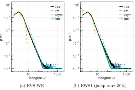
Figure 2. Power-law networks and random vertex based sampling (p= 0.2).
of the constructed undirected graphGi through w/( ¯d
i+w), where ¯di is the mean degree of
the graph. Finally, we note that typical sampling proportions p used in the literature vary between 0.1 and 0.3.
5.2. Synthetic directed networks. We generated 30 directed scale-free networks where the in-degree and the out-degree distributions follow a power law. The expected numbers of nodes, edges, in-degree exponent and out-degree exponent, are 105, 3×10⁵, 1.5 and 1.5, respectively. For each directed network, we estimated the in-degree distribution in the largest component using the inversion and asymptotic approaches under sampling methods with replacement. The proportionp of vertices (edges) sampled is 0.2 and the jump rate for the RWS algorithms is set to 30%.
Figures 2(a)–2(b) show the estimation results for RVS-WR and RWS1, respectively, where vertices are sampled uniformly (in the limit for the RW). The “true” line corresponds to the average of the p.m.f.’s of the 30 generated networks. The average of the estimates from the in-version approach with penalization (25)–(26), labeled “inv,” can recover the beginning (bulk) of the distribution with some bias for the in-degree zero. We note that without penalization, the variance of the unbiased estimator (15) is so large that the estimator of the distribution is impractical. The penalization parameterλin (25) has the effect of shrinking the estimates of the in-degree distribution, that leads to a substantial reduction in the variance, at the expense of increasing the bias. This approach also controls the variance in the tail by forcing the estimates to be equal to zero.
The comparison between Figures 2(a) and 2(b) shows that RWS1 with a moderate jump rate can approximate RVS-WR (which can be viewed as RWS1 with jumps only).
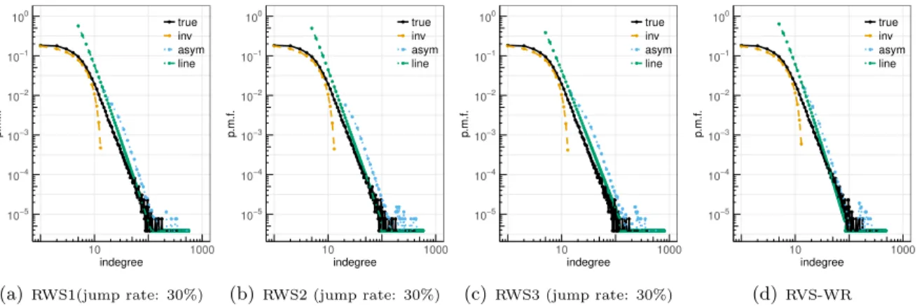
Figures 3(a)–3(c) present the (average) estimation of the in-degree distribution for RES-WR, RWS2 and RWS3, respectively, where edges are sampled uniformly (in the limit for the RWs). The inversion approach shows the same behavior as in Figure 2, with more bias for the smallest in-degrees in the case of the RWS. We note that the analysis developed in Section 4 for the LINE and ASYM methods is based on rescaling the tail of the sample in-degree distribution. For RWS1, the tail of the sample in-degree distribution tends to be smaller compared with RWS2/3 due to MH algorithm which avoids high-degree vertices; on the other hand the tail of the sample distribution tends to be smaller with RWS2 than with RWS3 because of the jumps of the former to random edges instead of vertices which somehow produce a more uniform sample (this explains the differences in Figures 2(b) , 3(b) and 3(c) for the LINE and ASYM methods). The ASYM method is accurate for large in-degree values. We also found that the estimation with the inversion approach for all sampling methods is less sensitive to changes in the jump rate than when using the asymptotic approach.
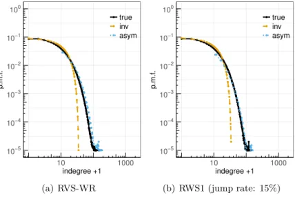
Figure 4 shows the (average) results of 30 generated random directed graphs with ex-ponential in-degree distribution for RNS-WR and RWS1, where we decreased the sampling probability and jump rate. The number of vertices and edges generated are the same as in the power-law networks above. Only the inversion and ASYM method are used to estimate the in-degree distribution. The inversion approach shows better performance over the power-law networks above due to the form of the p.m.f. at the beginning (decreasing slowly with the in-degree). A better fit is also shown with the ASYM method for the tail. We omit the plots for RES-WR and RWS2/3 but similar conclusions can be drawn.
5.3. Real-world directed networks. We examine here the suggested estimation methods on two real directed networks. The first network is the Amazon product co-purchasing net-work discussed in Section 1. Figures 5(a)-5(c) depict the performance of estimation using our RWS schemes on this network withp= 0.15 and jump rate 30%. Due to the particular form of the bulk of the in-degree distribution, the inversion method works well for the beginning of the distribution range. For the LINE method, the parameterα in (47) is estimated from the sample in-degree distribution (and the same for the HEP-PH network below). The discussion concerning the power-law networks in Section 5.2 above and more specifically on the differ-ences of the RWS schemes for the asymptotic approach applies here as well. For reference and for comparison to RWS1 in Figure 5(a), we also include in Figure 5(d) the estimation results for RWS-WR. When combined together, the inversion and asymptotic approaches approaches estimate the whole underlying in-degree distribution.
The second network is a citation network known as HEP-PH (high energy physics phe-nomenology) from the e-print arXiv originally described in Gehrke et al. (2003). The dataset covers all the citations in the area for a period of ten years withNv = 34,546 papers, Ne =
10−5 10−4 10−3 10−2 10−1 100
10 1000
indegree +1
p
.m.f
.
true inv asym line
(a) RES-WR
10−5 10−4 10−3 10−2 10−1 100
10 1000
indegree +1
p
.m.f
.
true inv asym line
(b) RWS2 (jump rate: 30%)
10−5 10−4 10−3 10−2 10−1 100
10 1000
indegree +1
p
.m.f
.
true inv asym line
(c) RWS3 (jump rate: 30%)
Figure 3. Power-law networks and random edge based sampling (p= 0.2).
10−5
10−4
10−3
10−2
10−1
100
10 1000
indegree +1
p
.m.f
.
true inv asym
(a) RVS-WR
10−5
10−4
10−3
10−2
10−1
100
10 1000
indegree +1
p
.m.f
.
true inv asym
(b) RWS1 (jump rate: 15%)
Figure 4. Non power-law network and random vertex based sampling (p= 0.15).
10−5 10−4 10−3 10−2 10−1 100 10 1000 indegree p .m.f . true inv asym line
(a)RWS1(jump rate: 30%)
10−5 10−4 10−3 10−2 10−1 100 10 1000 indegree p .m.f . true inv asym line
(b) RWS2 (jump rate: 30%)
10−5 10−4 10−3 10−2 10−1 100 10 1000 indegree p .m.f . true inv asym line
(c)RWS3 (jump rate: 30%)
10−5 10−4 10−3 10−2 10−1 100 10 1000 indegree p .m.f . true inv asym line (d)RVS-WR
Figure 5. Amazon network with RWS (p= 0.15).
10−4 10−3 10−2 10−1 100 10 1000 indegree +1 p .m.f . true inv asym line
(a) RWS1 (jump rate: 30%)
10−4 10−3 10−2 10−1 100 10 1000 indegree +1 p .m.f . true inv asym line
(b) RWS2 (jump rate: 30%)
Figure 6. ArXiv HEP-PH network (p= 0.1).
6. Discussion
The estimation of the in-degree distribution was formulated as a linear inverse problem, that involved a matrix dependent on the sampling scheme (RVS or RES) and relating the sample in-degree distribution to the true underlying in-degree distribution of the network. Due to the inherent difficulty in observing the node in-degree, the matrices of the sampling schemes tended to be ill-conditioned for small sampling rates. To deal with ill-conditioning, a penalized weighted least-squares estimation was proposed. An asymptotic approach was also developed to estimate directly the tail of the in-degree distribution. This analysis relied on a probabilistic asymptotic equivalence between the true and sampled in-degree distribution tails. It is much less computationally intensive than using inversion. Two asymptotic methods were presented: the LINE method which assumed a power-law behavior found in many real networks, and the ASYM method which was distribution free.
Finally, our simulations on synthetic networks of different topologies and applications to real networks showed that the inversion combined with the asymptotic approach can recovered the true in-degree distribution over its full range under sampling rates in the range 15%–20%. We found that the inversion approach was less sensitive to the RW sampling scheme and jump rate used. On power-law networks, the random walk which sampled nodes uniformly (RWS1) performed better in the estimation of the tail with the asymptotic approach, where jump rates of 30% seemed to work well in practice. The jump rates could be smaller in the case of non power-law networks.
As future problems related to this work, for example, it would be interesting to adapt the suggested methodology for quantities of interest in networks other than the in-degree distribution; to get a better sense of how the suggested methodology depends on network characteristics; or to use graph sketching (a sketch is a compact representation of data) in conjunction with sampling to infer even the same in-degree distribution.
Acknowledgment
I would like to thank Prof. Serhan Ziya and Prof. Shankar Bhamidi for introducing me to the fascinating world of statistical research. I would also thank Wang Bang, who is currently finishing his Ph.D. in statistics at University of Pittsburgh, for his contribution in this project. Finally, I offer my sincerest appreciation to Prof. Vladas Pipiras and Prof. Nelson Antunes for their guidance, expertise, and tolerating me.
Appendix A. Proof of the inverse matrix in Eq. (18)
We will throughout assume that the maximal in-degree J < nv, the number of samples.
Further to simplify notation, we writeN := Nv and n := nv. Recall the expressions of the
original matrixPs(·,·) from (16) and the corresponding asserted inversePs−1 from (18). The
assertion follows from the following two observations:
I. Diagonal entries of the product: For all 0≤k≤J one has Ps(k,·)Ps−1(·, k) = 1.
Proof: Using the expressions for the two matrices one has
Ps(k,·)Ps−1(·, k) = k k
N−k
n−k
N n
×
N−n−1
0
N
k
n k
= 1.
II. Off diagonal entries of the product: For allk1 6=k2