An Improved Technique for Multi-Dimensional Constrained Gradient Mining

(1)

AN IMPROVED TECHNIQUE FOR

MULTI-DIMENSIONAL CONSTRAINED GRADIENT MINING

O.J. ELUGBADEBO*1_{, A.S. SODIYA}2_{, O. FOLORUNSO}2

1_{Federal College of Education, Osiele, Abeokuta, Ogun State, Nigeria.} 2_{University of Agriculture, Abeokuta, Ogun State, Nigeria.}

[email protected], [email protected] *Corresponding author: [email protected]

businesses leverage the knowledge hidden in their own data by adjusting their business strategies accordingly.

Analyzing large amount of data collected through daily operation is a non-trivial task, let alone analyzing data from a dimensional point of view. Thus, multi-dimensional data analysis has been the focus of recent research in the field of data mining. It pursues a systematic approach in data analysis and helps businesses leverage the knowledge hidden in their own data by adjusting their business strategies accordingly (Tomasz et al., 2002). Also,

multi-ABSTRACT

Multi-dimensional Constrained Gradient Mining, which is an aspect of data mining, is based on mining constrained frequent gradient pattern pairs with significant difference in their measures in transactional database. Top-k Fp-growth with Gradient Pruning and Top-k Fp-growth with No Gradient Pruning were the two algorithms used for Multi-dimensional Constrained Gradient Mining in previous studies. How-ever, these algorithms have their shortcomings. The first requires construction of Fp-tree before searching through the database and the second algorithm requires searching of database twice in finding frequent pattern pairs. These cause the problems of using large amount of time and memory space, which retrogressively make mining of database cumbersome. Based on this anomaly, a new algorithm that combines Top-k Fp-growth with Gradient pruning and Top-k Fp-growth with No Gradient pruning is designed to eliminate these drawbacks. The new algorithm called Top-K Fp-growth with support Gradient pruning (SUPGRAP) employs the method of scanning the database once, by search-ing for the node and all the descendant of the node of every task at each level. The idea is to form projected Multidimensional Database and then find the Multidimensional patterns within the projected databases. The evaluation of the new algorithm shows significant improvement in terms of time and space required over the existing algorithms.

Keywords: Data mining, Association rules, Frequent itemsets, Multidimensional, Constraints,

Gradient.

INTRODUCTION

Data mining, also called Knowledge Dis-covery, is a multi-disciplinary field including database, artificial intelligence (especially machine learning) and statistics. In general, data mining is defined as the process of automatic extraction of implicit, novel, use-ful and understandable patterns in large da-tabases (Guozhu et al., 2001). The task of data mining, which is finding hidden and predictive information from large amount of data collected through daily operation, has been a major concern of today’s busi-ness world. Data mining pursues a system-atic approach in data analysis and helps

Journal of Natural Sciences, Engineer-ing and Technology ISSN - 2277 - 0593

(2)

change between two multi-dimensional enti-ties (patterns in transaction database).

The main objectives of this work are the technical issues of frequent pattern mining, identifying and analyzing algorithms for min-ing Multi-dimensional Constrained Gradient in Transactions database, developing an im-proved technique (SUPGRAP) that will combine two different pruning strategies: (support pruning and gradient pruning) as they are currently treated independently, test-ing and evaluattest-ing the new algorithm.

The rest of this paper is organized as fol-lows: section two presents review of existing literature on mining association rule in trans-actional databases. Section three discusses the improved algorithm. The implementa-tion and evaluaimplementa-tion were described in secimplementa-tion four. In section five, suggested future work were highlighted and the work is concluded in section six.

REVIEW OF LITERATURE Agrawal et al. (1993), mining association rules in databases has been a topic of choice among researchers. Since then, tremendous results have been recorded in developing different algorithms to mine frequent item-sets and association rules.

Frequent Pattern and Association Rule Mining

Frequent pattern mining is one of the achieve research themes in data mining. It is a process of applying data mining algorithm to find frequent patterns in a large database. The frequent pattern is a set of items that occurs frequently in a database (Ibrahim, 2004).

Association rule mining discovers interesting relationships among items in a given data set dimensional constraint gradient in

Transac-tional Database is basically used to correct the problem encountered in transactional database environment, most especially in finding pairs of frequent patterns with sig-nificant difference in their measures (Joyce Man, 2001).

Nowadays, data are usually collected in ta-bles stored in relational database systems. Each table has a schema. An attribute in the schema can be treated as a dimension. For example, a “Customer Category” attribute can be treated as a dimension with its own set of unique values and possibly a concept hierarchy for organizing values into differ-ent levels of granularity. Data having multi-ple dimensions can be arranged into a lat-tice of data cubes and viewed in a multi-dimension way. Similarly, in a transaction database, each tuple records the items (or products) bought in a transaction. Often it records other auxiliary information about a transaction such as the time the transaction happened and the location the transaction took place in. Attributes representing this auxiliary information can be treated as di-mensions. In this case we can view a trans-action as multi-dimensional. (Guozhu et al., 2001).

Constraints are user-specified conditions or restrictions that an answer must satisfy (Agrawal et al., 1993). There are restrictions indicating users’ interest in seeing what to report. Otherwise, returning a large answer set might overwhelm the users and report-ing unusable answers is a waste of computa-tion time.

In this work, we adopt the “gradient” defi-nition in a previous related work (Joyce Man, 2001) such that its magnitude, ex-pressed as a ratio of measures, indicates the

(3)

dominant time-consuming step. Thus, most research effort has been dedicated into find-ing efficient algorithms to mine frequent itemsets (or patterns). Below, we will discuss two influential algorithms, Apriori and FP-growth, in finding all frequent itemsets. For details in generating association rules from the frequent itemsets, please refer to (Agrawal et al., 1993).

Agrawal et al. (1993), Apriori has become the classic algorithm for finding frequent item-sets. With an iterative level-wise search ap-proach, it uses frequent k-itemsets to explore frequent (k+1)-candidate itemsets through join and prune steps. In general, first the set of frequent 1-itemsets, L1, is found. L1 is used to find the set of frequent 2-itemsets L2, which is used to find L3, and so on. This algorithm terminates when no further fre-quent k-itemsets Lk can be found. In the process of finding each Lk, one full scan of the database is required. To improve the effi-ciency of this iterative level-wise approach, the Apriori heuristic is used for pruning to nar-row down the search space. The anti-monotonic Apriori heuristic (Agrawal et al., 1994) states that if any length k pattern (itemset) is not frequent, its length (k+1) super-pattern can never be frequent. This is based on the observa-tion that if an itemset I do not satisfy the minimum support threshold, then I is not frequent and any superset of I will also be infrequent.

Ansari and Sadreddini (2009), in their re-search titled “An Efficient Approach to Min-ing Frequent Itemsets on Data Streams” which is also an aspect of this work used the approach “Sructured Frequent Itemsets on Data Streams (SFIDS) algorithm” for the implementation of Frequent Itemsets on Data Streams (FIDS) whereby the most fre-quent itemsets on data streams were derived (Guozhu et al., 2004). The basic concept can

be illustrated under the context of Market Basket Analysis. Imagine you are a retail store manager who wants to analyze your customers’ buying behavior. Let I = {i1, i2, …, im} be a set of items or products in your store. Let T be a set of task-relevant trans-actions where each t єT is a set of items such that t I. Each t has a unique trans-action identifier TID. Let A and B be item-sets, i.e. sets of items. (An item set is also called a pattern.) An item set containing k items is called a k-itemset. A transaction t contains an itemset A if and only if A t An association rule is of the form A => B with support s and confidence c where A I, B I and A ∩ B = Ø, where A and B are itemsets. Support s is defined as the percentage or absolute num-ber of transactions in T that contain A υ B, i.e. probability P (A υ B). Of all the transactions in T which contain A, confidence c indicates the percentage or absolute num-ber of these transactions which also contain B, that is the conditional probability P(B | A). To determine the interestingness of an association rule, minimum support thresh-old (min_sup) and minimum confidence threshold (min_conf) are used. An interest-ing or strong association rule must satisfy both minimum thresholds. Association rule mining is a two-step process Wang et al. (2006).

 Find all frequent itemsets (i.e. itemsets which occur at least in min_sup number of transactions). These frequent item-sets are also called large itemitem-sets (or pat-terns),

 Generate strong association rules from these frequent itemsets.

In this two-step process, the first step is the

∩

(4)

using one search method and it is one – di-mensional approach while our own proach tailored on multi – dimensional ap-proach because it involves two phases em-bedded in one algorithm called Support Gradient Prunning (SUPGRAP). The first phase involves searching for the most fre-quent itemsets in a transactional database and the second involves the extraction of the most profitable frequent itemsets from the resultof the first phase.

More often, there are some challenges in-herent in frequent pattern mining. There is a challenge of how to reduce the multiple scanning of the transaction database so as to improve system’s performance. There are challenges of how to reduce the massive number of candidates generated during the processes and to totally eliminate the tedi-ous workload of support counting of the generated candidates. These ideas lead to diverse options enhancements of the Apri-ori algApri-orithm (Nehinbe, 2004)

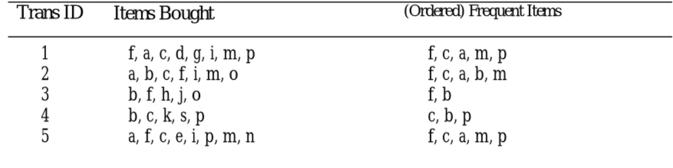
As described above, the disadvantages of Apriori algorithm are its expensive candi-date generation process that results in a huge number of candidates and the require-ment of scanning the entire database once at each level. Focusing on this weakness, FP -growth (Jiawei et al., 2000) minimizes the candidate generation process to only those most likely to be frequent and adopts a compact prefix tree data structure, FP-tree, to avoid repetitive scanning of the database. In this section, we examine FP-growth algo-rithm with an example since it is used in multi-dimensional constrained gradient mining in transaction databases (refer to Section 3). The following example is taken from (Jiawei et al., 2000) to illustrate the working of FP-growth. Assume transaction database T is shown in Table 1 and the

minimum support threshold is 3.

First, perform one scan of the transaction database T to find all frequent 1-itemsets. During scanning, frequency count for each item is tracked and compared with the mini-mum support threshold to determine if it is frequent. Only frequent items are of interest to us. Then we sort these frequent 1-itemsets in descending order of their frequency counts: <(f:4), (c:4), (a:3), (b:3), (m:3), (p:3)> (The number after “:” denotes the frequency count of an itemset. Then items in each transaction are sorted in this same order be-fore being inserted into the FP-tree, as shown in the column “(Ordered) Frequent Items”. This facilitates maximal sharing of nodes since items with higher frequencies appear closer to the root. Thus, the size of FP-tree created will be small. A second scan of T is required to create this compact FP-tree structure. After reading the first transac-tion, we insert each item into the tree and construct the first branch: <(f:1), (c:1), (a:1), (m:1), (p:1)>. After reading the second trans-action in T <f, c, a, b, m>, we find that it shares a common prefix path <f, c, a> with the existing branch <f, c, a, m, p> in the tree. Therefore, the count for each node in the prefix path is incremented by 1 and a new node (b:1) is created and linked as the child of node (a:2). Another new node (m:1) is created and linked as the child of (b:1). Figure 1 shows the FP-tree after insertion of two transactions.

Each subsequent transaction is scanned and inserted into the FP-tree. If a common pre-fix path already exists in the tree, the count in these common nodes are incremented. Otherwise, new nodes are created and in-serted into the FP-tree to accomplish inser-tion of a new transacinser-tion. Figure 2 shows the complete FP-tree for database T.

(5)

Table 1: Transaction table, with ordered frequent items

Trans ID Items Bought (Ordered) Frequent Items

1 f, a, c, d, g, i, m, p f, c, a, m, p 2 a, b, c, f, i, m, o f, c, a, b, m

3 b, f, h, j, o f, b

4 b, c, k, s, p c, b, p

5 a, f, c, e, i, p, m, n f, c, a, m, p

root

f: 1

a: 1 a:1

m:1

P:1

root

c: 2 f: 2

a: 2

b: 1 m:1

m:1 P:1

Figure 1: FP-tree after insertion of two transactions

(6)

root

f:4 c:1

c:3 b:1

a:3

p:1

p:2 m:2

b:1

m:1

Header Table

Item ID Node link

f

c

a

b

m

p

To facilitate tree traversal, a frequent-item header table is built during FP-tree construc-tion. Each entry consists of an item ID and the head of a node-link sequence to keep track of the first occurrence of each item in the tree. Items are arranged in descending frequency order in the header table. Each node in the tree has a link to the next oc-currence of the same item. By traversing this sequence of node-links, one can visit all occurrences of the same item in the tree. FP -growth mining algorithm starts with the

item having the least frequency count in the header table. In this example, we start with item as the initial suffix pattern. Imme-diately from the header table, we generate the frequent itemset <p:3>. By traversing the node links for item , we extract its prefix patterns, namely <f:2, c:2, a:2, m:2> and < c:1, b:1>. These prefix patterns form ’s conditional pattern base (i.e. the sub-pattern base under the condition of p’s exis-tence). Recursively, a conditional Fp-tree is con-structed for the suffix pattern, , based Figure 2: Sample FP-tree for database T

(7)

In summary, FP-growth algorithm only scans the whole database twice and mines on the compact data structure, FP-tree, to find all frequent itemsets without generating all possible candidate sets. Thus, FP-growth algorithm is a fast algorithm for mining fre-quent itemsets for association rule mining.

METHODOLOGY

Problem Definition

Informally, we can state the problem as “Given a frequent promotion pattern (fp) containing a set of promotion item(s) P and average profit of these promotion items in fp AvgProfitP(fp), we want to find the set of all frequent gradient patterns such that each frequent gradient pattern fg contains a set of items (including all promotion item(s) in P) and an AvgProfitP(fg) that is at least x% higher than that of fp’s.”(plural of fp )

Simple frequent pattern mining finds the complete set of frequent patterns F in a data-base. A frequent pattern f Î F is considered frequent (or significant) if it satisfies a signifi-cance constraint Csig (or support threshold). A frequent promotion pattern (fp) contains a set of promotion items defined by a k-conjunct of items, i.e. a promotion con-straint Cpro. Promotion constraint Cpro has the format of k-conjunct items = { id1 idk | k ≥1, idj єI} where I is a set of all unique items in T. Referring to our earlier example, Cpro = {TV}. This fre-quent promotion pattern fp is used as the basis for comparison with other potential frequent gradient patterns fg, which are super patterns of fp (i.e. fp fg). A gradi-ent constraint Cgrad is ex- pressed as a gradient function on frequent gradient pat-tern fg and frequent promotion pattern fp. It has the form

Cgrad(fg, fp) º g(fg, fp) θ v

where g is a gradient function, θ is a symbol on the conditional pattern base. This

condi-tional FP-tree only has one branch (c:3) be-cause only c is frequent by satisfying the minimum support threshold. Mining of ’s conditional FP-tree produces fre-quent 2-itemset (cp:3). Mining based on suffix pattern terminates. We move on to the next suffix pattern <m:3> in the header table. The conditional pattern base for suffix pattern <m> includes prefix paths <f:2, c:2, a:2> and <f:1, c:1, a:1, b:1>. Recursive mining of this conditional pattern base for <m> generates the frequent item-sets <am:3>, <cm:3>, <fm:3>, <cam:3>, <fam:3>, <fcam:3>, and <fcm:3>. In short, concatenating each frequent item in the conditional pattern base with the suffix pattern produces frequent itemsets of in-creasing lengths. Once mining of a suffix pattern has finished, we move on to the next more frequent item in the header table until the item with the highest frequency has been mined.

Mining starts from the item of least fre-quency in the header table because the con-ditional FP-tree generated for this least fre-quent item will still be compact since higher frequency items allow more sharing. All fre-quent itemsets with the least frefre-quent item, as the suffix pattern will be generated. Sub-sequently, conditional FP-trees for higher frequency items can ignore lower frequency items so that subsequent conditional trees are smaller in size. The compact FP-tree structure eliminates the need to have repetitive database scans in order to gener-ate candidgener-ate itemsets as in Apriori since all frequent itemsets must exist as a branch in the tree. As mining proceeds in this FP-tree, we only need to check if an itemset’s count meets the minimum support thresh-old.

>

(8)

m is a complex measure like AvgProfit of promotion items.

In subsequent sections, we first reason our choice on applying FP-tree/FP-growth to this problem instead of H-tree/H-cubing. Afterwards, we focus on each of the two steps involved in mining multi-dimensional constrained gradient patterns:

 Construction of Top-k FP-tree data structure;

 Mining results on Top-k FP-tree with Top-k FP-growth.

Top-k FP-growth with No Gradient Pruning algorithm

Since we use Top-k FP-tree as the data struc-ture, one simple method to solve multi-dimensional constrained gradient mining in transaction database is to adopt FP-growth algorithm on Top-k FP-tree (Joyce Man, 2001). Given promotion constraint Cpro, we find a set of promotion item(s) p є P, calcu-late AvgProfit(P) in transaction database and construct corresponding Top-k FP-tree. We apply FP-growth algorithm using signifi-cance constraint Csig as its support threshold to find a set of frequent patterns from Top-k FP-tree. This set of frequent patterns result-ing from pure support prunresult-ing is a superset of the set of frequent gradient patterns. Thus, an iterative post-processing step is re-quired to filter out patterns that do not sat-isfy the derived gradient pattern threshold Cgpat. We call this method Top-k FP-growth with No Gradient Pruning (TopkFpNoGP).

Top-k FP-growth with No Gradient Pruning

Algorithm (Top-k FP-growth with No Gradient Pruning)

Input: A multi-dimensional transaction

data-base T, a significance constraint Csig, a pro-of <, >,≤, ≥, etc. and v is a constant value.

A frequent gradient pattern fg must

 be frequent (or significant) based on sig-nificance constraint Csig,

 contains all promotion items defined in promotion constraint Cpro, and

 be Cgrad(fg, fp) = true.

We limit our study of gradient constraint to the ratio of fg’s and fp’s measures such that

Cgrad(fg, fp) = θ v

where m(f) is an arbitrary measure for a fre-quent pattern f. In this study, we focus on complex measures, e.g. m = AvgProfit of promotion items P = AvgProfit (P). (Joyce et al., 2001)

Let T be a multi-dimensional transaction database with schema S where S contains two non-overlapping sets of attributes: di-mensional attributes D and measure attrib-utes M, and a set of items bought together in a transaction. Let pattern be a set of items occurring together. Let fg be a gradi-ent pattern and fp a promotion pattern. Given a significance constraint Csig, a pro-motion constraint Cpro and a gradient con-straint Cgrad, find all valid gradient-promotion pattern pairs (fg, fp) in T such that

the set of promotion items p єP is defined by Cpro,

 fp is a frequent pattern containing all p Î P,

·fg and fp are frequent (or significant) pat-terns (i.e. satisfy Csig),

fg must be a superpattern of fp (i.e. fp fg),

fg’s measure, m(fg), must satisfy Cgrad, and

 

p g f m

f m

(9)

Method

1) Scan T once to get projected database on promotion item(s) P (based on Cpro) T’ and calculate AvgProfit(P) in T. Remove promo-tion item(s) from each transacpromo-tion t’ Î T’. Schema for T’ is mapped to:

T’ (# items in transaction, itemID,

…, itemID, profit(P)) where an itemID can be a unique dimension

value or an item bought in t’.

2) Scan T’ once to get frequent large-1 items using Csig.

3) If (number of large-1 items > 0)

a) Derive gradient pattern threshold Cgpat from Cgrad and AvgProfit(P) in T.

b) Calculate the number of bins re-quired using average and minimum profit of P and user-specified bin size.

c) Scan each transaction t’ Î T’ sec-ond time to construct Top-k FP-tree. d) Call Top-k-growth(top-k FP-tree, null) using Csig and Cgpat…..(ii)

Example (Top-k FP-growth algorithm)

Based on Top-k FP-tree constructed for Ta-ble 1, we know AvgProfit(Cg) ≥ Cgrad x AvgProfit(P) = 110, and Csig = 3. Let k = Csig = 3. Top-k FP-growth algorithm starts mining from the last item in header table, i.e. p. Pattern (p:3) is frequent with top-3 aver-age = actual averaver-age = (200+80+60)/3 = 113.3 ≥ 110 = Cgpat. So (p:3, 113.3) is a fre-quent gradient pattern which can form a gra-dient-promotion pattern pair with promo-tion items P. Since top-3 average of p passes Cgpat, we recursively construct conditional FP -tree for p and continue mining base on pre-fix pattern (p). As we can see, (cp: 3) is the only frequent pattern. Its top-3 average = actual average = 113.3 ≥ 110 = Cgpat so (cp: 3, 113.3) is also a frequent gradient pattern. Let’s skip to see how we mine Top-k FP-tree motion constraint Cpro, a gradient constraint

Cgrad, and size of each bin.

Output: The complete set of frequent

gra-dient patterns that can form valid gragra-dient promotion patterns satisfying all constraints with frequent promotion pattern fp that contains the set of promotion items P.

Method

1) Construct a Top-k FP-tree as described in section “Considerations for the new algorithm”

2) Apply FP-growth (as described in Chap-ter 2) on Top-k FP-tree using Csig as sup-port threshold.

3) Derive Cgpat using Cgrad and AvgProfit(P) in T.

4) FOR EACH frequent pattern f found DO // post-processing

{

a) If frequent pattern f’s AvgProfit(P) passes Cgpat threshold

i) Report as frequent gradient pattern fg }

However, this algorithm searches through fp tree which means it search from node to node before considering its descendants one after the other, because of this much of the user’s time is consumed. As a result of this drawback, Joyce Man, (2001) developed and implemented another algorithm called Top-k Fp-growth with Gradient Pruning (TOPFPGP) as described below:

Algorithm (Top-k FP-growth with Gra-dient Pruning)

da-tabase T, a significance constraint Csig,, a promotion constraint Cpro, a gradient con-straint Cgrad, and size of each bin

gra-dient-promotion pattern pairs that satisfy the three constraints.

(10)

need for the development of an improve al-gorithm that will address the inadequacies of the above discussed algorithms.

Considerations for the new algorithm

Having discussed the differences and inade-quacies of the first and second algorithm such that in searching for frequent pattern pairs there would be need for the algorithm to construct Fp-tree before searching through the database while the second algo-rithm requires searching of database twice, which retrogressively make mining of data-base cumbersome. Based on these anoma-lies, the hybrid prototype targets is to ensure that:

1. the scanning of database is carried out once and not twice as in the case of first and second algorithm.

2. there will be no need for the con-struction of Fp-tree before scanning the database.

3. user’s time in mining process is dras-tically reduced.

The New Algorithm-(Top-k FP-Support Gradient pruning)

Top-k FP-Support Gradient pruning is an improved technique for solving Multidimen-sional Constrained Gradient Mining prob-lems in Transactional Database. (i.e finding frequent pattern pairs). Giving promotion constraint Cpro, we find a set promotion item (s) pÎP. Derive gradient pattern threshold Cgpat from Cgrad and calculate Avgprofit(p) in transactional database. For each frequent pattern f found, form projected sional Database and then find Multidimen-sional patterns within the projected Data-bases in order to make scanning of database to be once. Compare the results to deter-mine whether the frequent pattern f’s Aver-age(p) will passes Cgpat threshold and to re-port finally whether the result form a fre-in Figure 3 from item f fre-in header table.

Pat-tern (f:4) is frequent with top-3 average = (200+100+60)/3 = 120 ≥ 110 = Cgpat. However, (f:4)’s actual average = (200+100+60+60)/4 = 105 ≥ 110 = Cgpat so even though (f:4) is frequent, it is not a frequent gradient pattern. Since (f:4) passes top-3 average, we continue mining its con-ditional FP-tree with prefix path (f).

Mining from the last item in Header Table f, pattern (cf: 3) is frequent with top-3 aver-age = actual averaver-age = (200+100+60)/3 = 120 ≥ 110 = Cgpat so (cf: 3, 120) is a fre-quent gradient pattern. Recursively mining the conditional FP-tree for prefix path (cf), we find pattern (acf: 3) is a frequent pattern with top-3 average actual average = (200+100+60)/3 = 120 ≥ 110 = Cgpat so (acf: 3, 120) is a frequent gradient pattern also. Next, we move on to item b in Header Table f, pattern (bf: 2) is not frequent so terminate searching for patterns with prefix path (bf). We move on to item a in Header Table f, pattern (af: 3) is frequent and top-3 average = actual average = 120 ≥110 =

Cgpat so (af: 3, 120) is a frequent gradient pattern.

The final answer of the complete set of fre-quent gradient patterns from Figure 1 is listed in Table 2.

According to Joyce Man (2001), in his final analyzes, he found that the second algo-rithm which was based on scanning of the database in order to enhance and comple-ment the performance of the first algo-rithm did not lived up to expectations. However, despite of the algorithm effi-ciency and performance when compare with the first prototype, research later reveal its inadequacies as the scanning of database is done twice. Hence, there is an urgent

(11)

quent gradient fg or otherwise.

da-tabase T, a significance constraint Csig,, a promotion constraint Cpro, a gradient con-straint Cgrad, and size of each bin

gra-dient-promotion pattern pairs that satisfy the three constraints.

Method

(1) Given the database (T) for all item set. i. If item set Csig then

ii. Frequent patterns = item set (2) Scan t once to get large frequent items

using bin size.

(3) If (large frequent items > 0)

Derive gradient pattern threshold Cgpat from Cgrad and AVGProfit (P) in T. (4) FOR EACH frequent pattern f found, form projected MD – Database and then find MD – Patterns within projected databases.

a. If frequent pattern f’s Average (P) passes Cgpat threshold

(i) Report as frequent gradient pattern fg ELSE

(ii) REPORT as No Frequent gradient pattern Nfg

Implementation evaluation

The new system was implemented using C# because of the support for interactive appli-cations.

Database Structure

The name and structures of Database are stated below:

SUPGRAP: It consists of two (2) main menus with additional command buttons on the toolbars, which serves as shortcut to all the menu items. Its General menu con-sists of authentic (real) data collected from supermarket stores are kept in this table. It



has the following fields:

Transactions Item Transactions Entry Items Report Transaction Report Exit

2. TRANSACTION ITEM:-Transaction Items menu is a table displays where the user can enter the various item products being sold and their unique ID’S. it has the following fields:

Unique ID Item Name Date Time

3 TRANSACTION ENTRY FORM:-

This is a table that allow the user gets to the screen where the various transactions can be entered on daily basis. It has the following fields:

Client Name Transaction Date Transac-tion Item Associated Profit

4. ITEMS REPORT:- This is a table that allow the user to get to the screen were the process criteria for generating report can be entered. It has the following field:

Period start period end Top-k Min. Length Prefix Item Constrained Gradient

5. TRANSACTION REPORT:- This is a table that shows the result of frequent gradi-ent patterns generated with their equivalgradi-ent Associated profit based on the selected proc-ess criteria. It has the following fields: Transactions (Frequent Gradient Patterns) Associated Profit (N) Date Time

Experiments

As discussed earlier, the performance of TopkFpNoGp, TopkFp and SUPGRAP al-gorithms are affected by several factors such as the Significant Constraint, Gradient

(12)

Con-straint, Number of Tuples, transaction and pattern length, pattern length specified. Hence, we take a closer look at how these factors actually affect the performance of the three algorithms to examine which, and under what situation, one is better than the other, taking into consideration the run-time speed and amount of memory used.

Evaluation Results

Results on Top-k FP-growth with Sup-port, Gradient and Support Gradient Pruning

For multi-dimensional constrained gradient mining in databases, we tested Top-k FP-Growth with No Gradient pruning (TopkFPNoGp), Top-k FP-growth with Gradient pruning (TopkFP) and Top-k FP-growth with Support Gradient Pruning (SupGrap). We conducted experiments on synthetic datasets generated from a syn-thetic transaction database.

In Figure 3, we tested the effect of signifi-cance constraint Csig on runtime. We fix gradient threshold Cgrad to 1.1, average transaction length to 12, average pattern length to 6. As we can see, when Csig de-creases, Top-k FP-growth with No Gradi-ent Pruning (TopkFPNoGP) requires sig-nificantly more time than Top-k Fp-growth with Gradient Pruning (TopkFP). And Top -k Fp-growth with Gradient Pruning (TopkFP) requires more time than Top-k Fp-growth with Support Gradient Pruning (SUPGRAP) which shows that Support Gradient Pruning is an improved method reason been that it out performs the other two methods. This is because without gradi-ent constraint pruning, the superset of fre-quent patterns quickly outgrows the subset of frequent gradient patterns. The time re-quired to mine the Top-k FP-tree increases

dramatically and the post-processing time required to filter the results also increases. Next we investigated the effect of gradient constraint Cgrad on algorithms’ runtime. We fix Csig to 25 (0.25% of total number of tu-ples) but range Cgrad from 1 to 10. From Figure 4, we conclude that Top-k FP-growth with Support Pruning requires pretty much a constant amount of time because the num-ber of frequent patterns is constant as Csig is fixed. However, Top-k FP-growth with Sup-port Gradient Pruning is better in perform-ance when compared with other two algo-rithms.

As shown in figure 5, we fix Csig, Cgrad and number of beans as we change the number of tuples. Intuitively, as the numbers of tu-ples increases, the runtime for three algo-rithms also increases. However, Top-kFP-growth with No Gradient pruning takes more time than Top-kFP-growth whileTop-kFP-growth with support Gradient pruning takes lesser compare to other two algorithms as the number of tuples increases. This is to the increase in the number of frequent pat-terns satisfying Csig and thus more time in mining those frequent patterns that may sat-isfy Cgrad.

For transaction databases, we also performed an experiment to determine the effect of average transaction length and average pat-tern length. First, we test the effect of aver-age transaction length by generating multiple datasets of size 10,000 tuples with different average transaction lengths. Note that we fix the average pattern length to be half of aver-age transaction length such that the frequent patterns length we mine increases with aver-age transaction length. In Figure 6, we can see as the average transaction (and thus, pat-tern) length increases, both algorithms

(13)

re-quire more time to mine longer frequent gradient patterns as expected. The gradient pruning strategy in Top-k FP-growth Sup-port Gradient Pruning algorithm performs better than Top-k FP-growth with Gradient Pruning and this also performs better than Top-k FP-growth with Support Pruning since more search space is pruned.

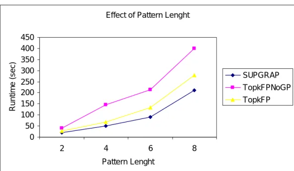
In Figure 7, we then showed the effect of average pattern length on runtime of both algorithms. As expected, when average pat-tern length increases, the amount of time to mine longer frequent patterns increases. The runtime for Top-k FP-growth with No Gradient Pruning increases significantly since other two uses gradient constraint for pruning to decrease the number of frequent patterns generated but Top-k FP-growth with support Gradient Pruning use lesser time compare to others.

FUTURE WORK

This work confirms our recognition of the potential in constrained gradient analysis. We see that further research effort is worth investing into this problem area in order to solve more related problems. Some of the suggested future works are:

1. Instead of returning the complete an-swer set, the algorithm can be modified to generate and rank the best-N answers that maximize the difference in meas-ures. This helps users to easily under-stand the result.

2. Based on current definition of the prob-lem, users must identify the items of interest for promotion, i.e. the promo-tion items. This suits the scenario when a user is looking to promote particular items based on festivities, inventory status and item popularity. Instead the algorithm can be modified to suggest an

item category for promotion and identify the cross-selling items to achieve the most profit.

3. Investigating into the possibility of using CLOSET algorithm (Jiawei et al., 2000) to mine a closet set of pattern pairs.

CONCLUSION

In this work, an improved algorithm and data structure were proposed to solve the problem in transaction database environment. The original FP-tree was modified to become a Top-k FP-tree data structure for storing aver-age measure information of transactions. FP-growth algorithm was enhanced to suit the Top-k FP-tree data structure. Integrating gra-dient constraint into processing, Top-k FP-growth with Support Gradient algorithm is more effective in its pruning strategy than Top-k FP-growth with Gradient Pruning and Top-k FP-growth with Support Pruning algo-rithm.

This work has been used to solve problem on multi-dimensional constrained gradient min-ing in transactional database. Combinmin-ing FP-growth and H-cubing algorithms and their corresponding data structures, FP-tree and H -tree respectively, we propose a Top-k FP-growth algorithm on a top-k FP-tree hybrid data structure for mining multi-dimensional constrained gradients in transaction data-bases.

With increasing competition in the business world, leveraging company data to give a competitive advantage is a sensible and im-portant step of survival. The direct applica-tion of this problem in the business paradigm warrants the significance of this research ef-fort. Experimental evaluations in this paper bring promises to this area. Our proposed algorithms successfully and efficiently extract multi-dimensional entity pairs that have sig-nificance difference in their measures.

(14)

(p) (p: 3, 113.3), (cp: 3, 113.3)

(m) (m: 3, 120), (fm: 3, 120), (cfm:3, 120), (afm:3,120), (acfm:3, 120), (cm:3, 120), (acm:3, 120), (am:3, 120)

(f) (cf:3, 120), (acf:3, 120), (af:3, 120) (c) (c:4, 110, (ac:3, 120)

(b) NONE (a) (a:3, 120)

Table 2: Result of frequent gradient patterns of figure 1

Mining with prefix path as… Resulting frequent gradient patterns...

Effect of Significance Constraint

0 100 200 300 400 500 600

25 30 35 40 50 100 150

Significance Constraint

R

u

n

ti

m

e

(

s

e

c

)

SUPGRAP TopkFPNoGP TopkFP

(15)

Effect of Gradient Constraint

0 50 100 150 200 250 300 350

1 1.1 1.2 1.5 2.2 5 10

Gradient Constraint

R

u

n

ti

m

e

(

s

e

c

)

SUPGRAP TopkFPNoG P

Figure 4: Effect of Gradient Constraint

Effect of Number of Tuples

0 200 400 600 800 1000 1200 1400 1600

10 20 40 50 60 80 100

# Tuples (k)

R

u

n

ti

m

e

(

s

e

c

)

(16)

EFFECT OF TRANSACTION AND PATTERN LENGHT

0 100 200 300 400 500 600 700

6\3 8\4 10\5 12\6 14\7 16\8 18\9 20\10

Transaction/Pattern Lenght

R

u

n

ti

m

e

(s

e

c

)

Figure 6: Effect of Transaction and Pattern Lengths

Effect of Pattern Lenght

0 50 100 150 200 250 300 350 400 450

2 4 6 8

Pattern Lenght

R

u

n

ti

m

e

(

s

e

c

)

(17)

REFERENCES

Agrawal, R., Ramakrishnan, S. 1994. Fast

Algorithms for Mining Association Rules. In Proceedings of the 20th International Conference

on Very Large Data bases (VLDB’04), Santiago,

de Chile, Chile.

Agrawal, R., Imielinski, T., Swami, A.

1993. Mining Association Rules between Sets of Items in Large Databases. In Proceedings of

the ACM SIGMOD Conference on Management of Data (SIGMOD’93), P. 207-216, Washington,

D.C.

Guozhu Dong, Jiawei Han, Joyce M.W. Lam, Jian Pei, Ke Wang 2001. Mining

Mul-tidimensional Constrained Gradients in Data

Cubes. To appear in Proceedings of 27th

In-ternational Conference on Very Large Data Bases (VLDB’01), September 11-14, 2001, Roma, Italy.

Guozhu Dong, Jiawei Han, Joyce M.W. Lam, Jian Pei, Ke Wang, Wei Zou 2004.

"Mining Constrained Gradients in Large Da-tabases," IEEE Transactions on Knowledge and

Data Engineering, 16(8): 922-938.

Ibrahim, S.A. 2004. An Efficient pattern

Growth Mining of Closed Frequent Itemsets: A thesis Submitted in Fulfilment of the re-quirement for the Degree of Master of ence in the Department of Mathematical sci-ences, University of Agriculture, Abeokuta.

Jian Pei, Jiawei Han 2001. Can we push

more Constraints into Frequent Pattern Min-ing?.In Proceedings of 6th ACM SIGKDD

Inter-national Conference on Knowledge Discovery and Data Mining (KDD’00), p.350-354, August

20-23, 2000, Boston, MA, USA.

Jian Pei, Jiawei Han, Laks V.S.

Lakshmanan 2001. Mining Frequent

Item-sets with Convertible Constraints. In:

Proceed-ings of the 17th International Conference on Data Engineering (ICDE’01), April 2-6, 2001,

Heidel-berg, Germany.

Jiawei Han, Jian Pei, Yiwen Yin 2000.

Min-ing Frequent Patterns without Candidate Gen-eration. In Proceedings of the 2000 ACM

SIG-MOD International Conference on Management of Data (SIGMOD’00), May 16-18, 2000, Dallas,

Texas, USA.

Joyce Man Wing Lam 2001:

Multi-dimensional Constrained Gradient Mining. A Thesis Submitted in Partial Fulfillment the Re-quirement for the Degree Master of Science in the School of Computing Science: Simon Fra-ser University.

Neinbe, O.J. 2004. Mining Frequent

MAX-Sequential patterns from Customer Portifolio – Database: A thesis submitted in Fulfilment of the requirement for the Degree of Master of science in the Department of Mathematical sciences, University of Agriculture, Abeokuta.

Ansari, S., Sadreddini, M.H. 2009. An

Effi-cient Approach to Mining Frequent Itemsets on Data Streams. In: Proceedings of World

Acad-emy of Science, Engineering and Technology, 37:

ISBN 2070-3.

Tomasz Imielinski, L. Khachiyan, A. Ab-dulghani 2002. “Cubegrades: Generalizing

Association Rules,” Data Mining and Knowledge

Discovery, 6: 219-258.

Wang, J., Han, J., Pei, J. 2006. Closed

Con-strained Gradient Mining in Retail Databases,

IEET Transactions on Knowledge and Data Engi-neering, 18(6): 764-769.