Sharif University of Technology
Scientia IranicaTransactions A: Civil Engineering www.scientiairanica.com
A one-parameter controlled dissipative unconditionally
stable explicit algorithm for time history analysis
S.-Y. Chang
, N.-C. Tran, T.-H. Wu and Y.-S. Yang
Department of Civil Engineering, National Taipei University of Technology, NTUT Box 2653, No. 1, Section 3, Jungshiau East Road, Taipei 10608, Taiwan, Republic of China.
Received 9 December 2015; received in revised form 12 May 2016; accepted 25 July 2016
KEYWORDS Unconditional stability;
Numerical dissipation; Explicit method; Nonlinear dynamic analysis;
Accuracy;
Structure-dependent integration method.
Abstract. A new family of one-step integration methods is presented herein. A free parameter is used to control the numerical properties and it can be considered as an indicator of numerical dissipation for the high-frequency modes. This family of methods can have unconditional stability, explicit formulation, and desired numerical damping, which implies that the low-frequency modes can be accurately integrated while the spurious growth of high-frequency modes can be suppressed or even eliminated. In addition, a zero damping ratio can be achieved. Since the unconditional stability and explicit formulation are integrated for the proposed method family, it can drastically reduce the computational eorts when compared with the traditional integration methods.
© 2017 Sharif University of Technology. All rights reserved.
1. Introduction
Many dissipative integration methods have been pro-posed for structural dynamics, such as the Houbolt method [1], Newmark method [2], Wilson- method [3], HHT- method [4], WBZ- method [5], generalized-method [6], Bathe generalized-method [7], Zhou and Tamma meth-ods [8-9], Rezaiee-Pajand and Alamatian method [10], Gholampour and Ghassemieh method [11], and quartic B-spline method [12]. All these integration methods are implicit and, thus, they will involve an integration procedure for each time step in conducting time inte-gration. It is well recognized that the nonlinear itera-tions for each time step will cost many computational eorts. On the other hand, if an integration method is explicit [2,10,13,14], it has conditional stability; thus, a very small time-step size may be required to satisfy
*. Corresponding author. Tel.: +886-2-2771-2171; Fax: +886-2-2781-4518
E-mail address: [email protected] (S.-Y. Chang) doi: 10.24200/sci.2017.4158
the upper stability limit. Consequently, it will be very promising if these dissipative integration methods can be enhanced with an explicit formulation for implementation. The structure-dependent integration method was rst developed by Chang in 2002 [15]. Some integration methods of this type were also successfully developed by Chang [16-22] subsequently. These structure-dependent integration methods can simultaneously integrate the major advantages of the implicit and explicit algorithms, i.e. the unconditional stability of implicit algorithms and no nonlinear itera-tions of explicit algorithms. However, they possess no numerical dissipation.
It is valuable to propose an integration method that possesses the desired numerical properties, which are unconditional stability, second-order accuracy, ex-plicit formulation, and favorable numerical dissipation. Two family methods [20,23] have been developed for this purpose. However, they are two-step methods and, thus, a distinct starting procedure is generally needed for practical applications. Both family methods are expressed by the three parameters , , and and their numerical properties are dominated by these three
parameters. In this work, a new family method is proposed. This family method is a one-step method and, thus, it is self-starting. In addition, its numerical properties are controlled by a free parameter, p, which can be considered as an indicator variable for numerical dissipation. The numerical properties of this family method are evaluated herein and some numerical ex-amples are examined to conrm the analytical results. 2. Proposed family method
In structural dynamics or earthquake engineering, the equation of motion of the discrete model can be expressed by a set of second-order ordinary dierential equations as:
mu + c _u + ku = f; (1) where m, c, k, and f are the mass, viscous damping coecient, stiness, and external force, respectively; and u, _u, and u are the displacement, velocity, and acceleration, respectively. This equation can be solved by many available step-by-step integration methods. A new family method is also proposed for solving this equation of motion. In order to develop the new family method, some basic assumptions are made for this development. Since the structure-dependent dierence equation for displacement increment plays a key role to integrate the unconditional stability and explicit formulation, it is adopted. In addition, this dierence equation is assumed to be a function of data of the previous step only since a one-step method is supposed to be developed. On the other hand, an asymptotic form of the equation of motion is assumed since it has been applied to develop some dissipative integration methods such as HHT- method and method. As a result, the proposed family method can be expressed as:
2
p + 1mai+1+ p 1
p + 1mai+ cvi+1+ ki+1di+1 = fi+1;
di+1 = di B12idi+ B2(t)vi+ B3(t)2ai;
vi+1=vi+2(p + 1)3p 1 (t)ai
p 3
2(p + 1)(t)ai+1; (2) where di, vi, ai, and fi are the nodal displacement,
velocity, acceleration, and external force at the ith time step, respectively; t is step size and kiis the stiness
at the end of the ith time step. In addition, i =
!i(t); and !i = pki=m is the natural frequency of
the system at the end of the ith time step, ki. Notice
that cvi+1+ ki+1di+1 in the rst line of Eq. (2) can
be rewritten as N(vi+1; di+1) for a general nonlinear
system [24]. The coecients B1 to B3 are:
B1=4D1
2 p + 1
2
;
B2=D1
2 p + 1+
3 p p + 1
1 2
2 p + 1
2
0
B3=D1
p (p + 1)2
1 2
p 1 p + 1
2 0
; (3)
where:
D =p + 12 +3 pp + 10+
1 p + 1
2
2
0; (4)
where is a viscous damping ratio; 0 = !0(t); and
!0 =
p
k0=m is the natural frequency of the system
determined from the initial stiness of k0. Notice that
i = 0 and !i = !0 are found for i = 1; 2; 3; :::
for a linear elastic system. The development details of this method are similar to those of the previously published algorithms [17,18] and, thus, they will not be elaborated on herein. In this derivation, the proof of convergence must be conducted rst. Hence, the requirements of the order of accuracy and uncondi-tional stability of the proposed family method are used to determine the coecients B1 to B3 appropriately.
This work is very complicated. The order of accuracy is determined from the local truncation error of the proposed family method. On the other hand, the procedure given by Lambert [25] and then invoking the Routh-Hurwitz criterion can be applied to determine the unconditional stability. Notice that p is the free parameter to govern the numerical properties. It will be shown later that p can be considered as the spectral radius of the proposed family method in the limit 0! 1 for a linear elastic system.
For computational eciency, it is very important to rewrite 0and 20in terms of the initial structural
properties and step size for a structure-dependent integration method. Thus, based on the theory of structural dynamics, the relations 2
0 = (t)2(k0=m)
and c0= 2!0m can be obtained as it is assumed that
viscous damping ratio, c0, is determined from the initial
structural properties. After substituting these relations into Eqs. (3) and (4), they become:
B2= D1
2 p + 1m
(p2 2p 1)
2(p + 1)2 (t)c0
; B3= D1
2 (p + 1)2m
1 4
p 1 p + 1
2
(t)c0
; D =p + 12 m+2(p + 1)3 p (t)c0+
1 p + 1
2
(t)2k 0:
(5) Notice that the coecients B1, B2, and B3depend only
on the initial properties of the structure and step size. Hence, they will remain invariant and, thus, there is no need to re-compute these coecients during a whole step-by-step integration procedure.
3. Recursive matrix form
Since the numerical properties of PFM can be derived from the characteristic equation of its amplication matrix, it is needed to rewrite Eq. (2) in a recursive matrix form. Thus, the use of PFM to obtain the free vibration in a system with single degree of freedom can be expressed in the following form:
Xi+1= AXi= A(i+1)X0; (6)
where Xi+1 = di+1; (t)vi+1; (t)2ai+1T is dened
and A is an amplication matrix. Notice that the vector X0 is in correspondence with the given initial
conditions d0 and v0. The initial acceleration can be
determined by a0 = (f0 cv0 kd0)=m. The explicit
expression of the amplication matrix A for a linear elastic system is found as shown in Box I, where B is further dened as:
B = p + 12 +3 pp + 10: (8)
Thus, the characteristic equation of the amplication matrix, A, can be obtained from jA Ij = 0 and is found to be:
3 A
12+ A2 A3= 0; (9)
where is an eigenvalue of the amplication matrix A and the coecients A1, A2, and A3 are found to be:
A1= 2p +(p + 1)D3p + 5 +2(2 p)D 0;
A2= p + 2 +( p
2+ 2p 5)
(p + 1)D 0 +(p 1)(p + 2)(p + 1)2D 2
0;
A3= (p + 1)D(p 1) : (10)
Notice that the characteristic equation can be applied to evaluate the numerical properties of PFM.
4. Convergence
The convergence of a computational method is implied by the consistency and the stability based on the Lax equivalence theorem [24]. In general, the consistency is dened by a qualitative measure, such as the order of accuracy, which can be directly determined from the local truncation error. In general, an algorithm is said to be convergent if it is both consistent and stable. 4.1. Consistency and local truncation error A local truncation error is dened as the error com-mitted in each time step by replacing the dierential equation with its corresponding dierence equation [26-28]. The approximating dierence equation for PFM can be obtained from Eq. (6) after eliminating velocities and accelerations and is found to be:
di+1 A1di+ A2di 1 A1di 2= 0: (11)
Consequently, after replacing Eq. (1) by Eq. (11), the local truncation error for PFM is:
E =(t)1 2
u(t + t) A1u(t) + A2u(t t)
A3u(t 2t)
: (12)
In addition, if u(t) is assumed to be continuously dierentiable up to any required order, the terms of
A = D1 2 6 6 6 6 4
B(1 B120) BB2 BB3
p 3
2(p+1)(1 B120)20 p+12 2(p+1)3 p B220 12 2(p+1)3 p B320
(1 B120)20 20 B220 p 1p+1 3p 1p+10 B320
3 7 7 7 7
5 (7)
u(t+t), u(t t), and u(t 2t) can be expanded into nite Taylor series at t. As a result, after substituting A1, A2, and A3 into the result of Eq. (11), the local
truncation error for PFM is found to be: Ei+1=
2 0!02
12(p + 1)2D
4(p + 1)(5p 7)2
(p2+ 2p 7)u i+ 4
2(p + 1)(5p 7)2
3(p2 3)u i
+ O(t)3;
(13) for a linear elastic system. This equation reveals that PFM has the minimum order of accuracy of 2 if Rayleigh damping is adopted and, thus, its consistency is veried for any values of p and any viscous damping ratio .
4.2. Stability
The stability analysis of PFM is very dicult by using an algebraic method. This is because it has three non-zero eigenvalues due to A3 6= 0. Alternatively, the
stability conditions will rst be considered for the two especial cases of 0 ! 0 and 0 ! 1 and, then,
a general value of 0 is studied. After nding the
coecients A1; A2; and A3 for the case of 0 ! 0,
Eq. (9) becomes: ( 1)2 +p 1
2
= 0: (14)
This equation reveals that PFM has two principal roots of 1;2= 1 in addition to a spurious root of 3= (p
1)=2. Apparently, these eigenvalues are independent of . To satisfy the stability condition, the value of 3
must be in the interval of 1 3 1. As a result,
1 p 3 is obtained. Similarly, in the limit of 0! 1, Eq. (9) is reduced to:
( + p)2= 0; (15)
where two principal roots are 1;2 = p and the
spurious root is 3 = 0. This implies that 1 < p 1
must be met for any viscous damping (p cannot be 1 because p = 1 leads some factor to be innity).
After obtaining the range of 1 < p 1 for PFM to have unconditional stability in the limiting cases of 0 ! 0 and 0 ! 1, it is needed to further conrm
that if the same range is applicable to a general value of 0. This can be evaluated by using the Routh-Hurwitz
criterion, which gives necessary and sucient condition for the roots of Eq. (9) to lie within or on the circle of
jj = 1 if the following inequalities are satised: 1 A1+ A2 A3 0; 3 A1 A2+ 3A3 0;
3 + A1 A2 3A3 0; 1 + A1+ A2+ A3 0;
1 A2+ A3(A1 A3) 0: (16)
After substituting Eq. (10) into Eq. (16), it is found that all the ve inequalities will be met if 1 < p 1 holds; this proves the stability of PFM. This stable property in conjunction with the previous proof of consistency implies the convergence of PFM.
5. Numerical properties
It is generally recognized that the spectral radius, relative period error, numerical damping, and over-shooting are the numerical properties of PFM, which will be further investigated herein. The techniques for evaluating these numerical properties can be found in the references [26,28,29] and, thus, will not be elaborated on here.
5.1. Spectral radius
The variations of spectral radii with t=T0, where T0=
2=!0, are shown in Figure 1 for p = 1:0; 0:5; 0; 0:5,
and 0:99. The spectral radius is the maximum absolute eigenvalue of the amplication matrix. For a small value of t=T0, the spectral radius is almost equal
to 1.0 for each curve; while, for a larger value of t=T0,
it decreases gradually and tends to a certain value. Notice that it is always equal to 1.0 for p = 1. This means that PFM can have zero damping for p = 1. At rst glance, it seems that the value of p can be chosen to be either in the range of 1 < p 0 or 0 p 1 since both ranges can provide appropriate numerical damping. However, it is worth noting that the curve for p = 0:5 shows an abrupt change of slope at the point (0.24, 0.62) as shown in Figure 1. This point might be a bifurcation point, where complex conjugate roots bifurcate into real roots.
Figure 1. Variations of spectral radius with t=T0 for
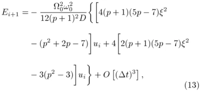
Figure 2. Principal roots of PFM with p = 0:5.
In order to clarify the dierence between the ranges of 1 < p 0 and 0 p 1 with respect to period distortion, the eigenvalues of PFM for the case of p = 0:5 are calculated and plotted in Figure 2. It is evident that the imaginary part of each principal root will become zero after the value of t=T0 grows
greater than around 0.67, as marked by a solid circle in the gure. This conrms that the complex conjugate roots bifurcate into real roots at this bifurcation point. In general, the two real roots imply that the obtained response is in an exponential decay form and there is no bounded oscillatory response, which is generally pre-ferred for an integration method. Further calculations reveal that a bifurcation point is generally found in the range of 1 < p < 0, which is of no interest for practical applications. Accordingly, the following study will focus on the range of 0 p 1 for PFM.
5.2. Relative period error
Figure 3 illustrates the relative period error of ( T0
T0)=T0 against t=T0 for p = 1:0; 0:75, 0.75, and
0.0. In addition, the results for the HHT- method and WBZ- method are also plotted in this gure for comparison. In general, the relative period error
Figure 3. Variations of relative period error with t=T0
for PFM.
increases with increase in t=T0 for each curve. It
is interesting to note that the curve of PFM with p = 1 almost coincides with that of HHT and WBZ as = 0. This phenomenon is likely to be found for PFM with p = 0:75, HHT with = 1
6, and WBZ with
= 0:143. Although the curve of PFM with p = 0 seems to overlap with that of WBZ with = 0:333, both methods show more period distortion than that of HHT with = 1
3. However, the dierence in
period distortion among the three family methods is not very signicant for a small value of t=T0, say
t=T0 0:05.
It is found that a large value of p will lead to a small relative period error for a given value of t=T0.
It has been considered as a good rule of thumb for choosing t=T0 0:05 to yield a reliable response [27].
This criterion indicates that the range of 0:5 p 1 might be of great interest for practical applications, since PFM with a p value in the range of 0 p 0:5 seems to result in too much period distortion.
5.3. Numerical damping
The numerical damping ratio can be applied to evaluate the numerical dissipation of a time integration method Figure 4. shows the variation of numerical damping ratio versus t=T0 for PFM with p = 1, 0.75, and
0.0. For each curve, the numerical damping ratio is very small for a small value of t=T0 and, then, it
increases gradually; nally, it becomes constant. In this gure, it is also found that the numerical damping ratio is controlled by the p value only, where p = 0 gives the highest numerical damping ratio and p = 1 leads to zero damping. In general, a large value of p value will result in a small numerical damping ratio for a given value of t=T0. This gure also implies
that PFM with a p value in the range of 0 p 0:5 may lead to very large numerical dissipation for low frequency modes since PFM with p = 0 has a numerical damping ratio of 2% for t=T0= 0:05.
For comparison, the results for HHT and WBZ are also plotted in Figure 4. In general, zero damping
Figure 4. Variations of numerical damping ratio with t=T0for dierent values of p.
is achieved for PFM with p = 1, HHT with = 0, and WBZ with = 0. It is also found that the curves for PFM with p = 0:75 and 0.50 almost overlap with those for WBZ with = 0:143 and = 0:333, respectively. Notice that PFM with p = 0:5 and WBZ with = 0:333 will result in the maximum numerical damping ratios, which are generally larger than those of HHT with = 1
3.
In Figure 1, it is found that in the limit of 0! 1
(or t=T0 ! 1), the spectral radius is convergent on
the p value. In fact, the spectral radii for p = 1:0, 0.5, and 0.0 are found to be 1.0, 0.5, and 0.0, respectively, in the limit of 0 ! 1. On the other hand, Figure 4
reveals that a large p value leads to a small numerical damping ratio. Consequently, the free parameter, p, might be considered as an indicator variable of numerical dissipation for high-frequency modes. As a result, a value of p close to 1 implies a small numerical damping for high-frequency modes while a value of p close to 0 indicates a large numerical damping for high-frequency modes. In summary, a small p value will lead to a large numerical damping ratio while it accompanies a large relative period error.
5.4. Overshooting
In order to evaluate the tendency of an integration method to overshoot the exact solutions in the early response [30,31], the free vibration response of a linear elastic single-degree-of-freedom model problem is often considered. In general, it can be expressed as:
u(t) + !2u(t) = 0; (17)
with initial conditions u(0) = d0and _u(0) = v0. Since
PFM is a converged method, there is no overshoot as 0 ! 0. In general, 0 ! 1 can provide an
indication of the overshooting behavior of the high-frequency mode in a system where the values of t=T0
are large for the high-frequency mode. As a result, the following equations can be obtained for the limiting condition of 0! 1:
di+1 pdi;
vi+1 14(p 1)220
di
t
+
1
2(p 1)2 1
vi:
(18) The rst line of this equation reveals that there is no overshooting in displacement for any member of PFM while it has a tendency to overshoot quadratic 0 in
the velocity equation due to the initial displacement term as indicated by the second line of this equation (U0-V1). Interestingly, the overshooting velocity dis-appears and becomes U0-V0 for p = 1.
In order to conrm the analytical prediction of the overshooting behavior of PFM, the free vibration
Figure 5. Comparison of overshooting responses.
response of a single-degree-of-freedom system is calcu-lated by using a relatively large time step. In fact, it is computed by using PFM with p = 1, 0.5, and 0 and AAM with a time step corresponding to t=T0= 10 for
the initial conditions of d0= 1 and v0= 0. Numerical
results are shown in Figure 5, where the velocity term is normalized by the natural frequency of system in order to have the same unit as that of displacement. The horizontal axis measures time in a number of time steps. It is manifested in the top plot of Figure 5 that all the three curves for PFM exhibit no overshoot in displacement. In addition, the curve for PFM with p = 1 coincides with that of AAM. A signicant overshoot in velocity is found in the bottom plot of this gure for p = 0:5 and 0 although it is almost annihilated in the rst few time steps. Again, the two curves for PFM with p = 1 and AAM overlap. This implies that PFM with p = 1 has the same overshooting behaviors as those of AAM for a linear elastic system. As a result, these numerical results are in good agreement with the analytical results.
6. Implementation details
For the applications of PFM to solve a multiple-degree-of-freedom system, the implementation of PFM is presented next. The general formulation for PFM can be written as:
2 p + 1
Mai+1+
p 1 p + 1
Mai+ C0vi+1
+ Ki+1di+1= fi+1;
di+1=
I B1(M 1Ki)(t)2
di+(t)B2vi+(t)2B3ai;
vi+1= vi+ (t)
3p 1 2(p + 1)ai+
3 p 2(p + 1)ai+1
; (19) where M is a mass matrix, C0 is a constant damping
matrix and is assumed to be determined from the initial structural properties, and Ki is the stiness matrix
at the end of the ith time step; di, vi, ai, and fi
are the nodal vectors of the displacement, velocity, acceleration, and external force, respectively; and I is an identity matrix with the size of n n, where n is the total number of degrees of freedom of the system. The coecient matrices of B1 to B3 and D are found
to be:
B1= (p + 1)1 2D 1M;
B2= D 1
2 p + 1M
(p2 2p 1)
2(p + 1)2 (t)C0
; B3= D 1
2 (p + 1)2M
(p 1)2
4(p + 1)2(t)C0
; D=p + 12 M+2(p + 1)3 p (t)C0+(p + 1)1 2(t)2K0;
(20) where K0 is the initial stiness matrix of the system.
It is generally dierent from the stiness matrix, Ki,
in Eq. (19) for a nonlinear system. It is important to note that the coecient matrices B1 to B3 must be
determined from the initial structural properties of M, C0, and K0 as well as the step size before performing
the time integration.
At the start of the (i + 1)-th time step, the displacement vector can be computed by using the second line of Eq. (19). It is numerically equivalent to the outcome of following equation:
D(di+1 di) = (p + 1)1 2(t)2ri
+
2 p + 1M
(p2 2p 1)
2(p + 1)2 (t)C0
(t)vi
+
p (p + 1)2M
(p 1)2
4(p + 1)2(t)C0
(t)2a
i:
(21) After obtaining the current displacement vector, the assumed force-displacement relations can be applied to determine the corresponding restoring force vector. In general, ri+1= Kdi+1is used to represent the restoring
force vector. Subsequently, the velocity vector, vi+1,
can be calculated by substitution of the third line of Eq. (19) into the rst line of this equation. As a result, the resultant equation is numerically equivalent to the outcome of the following equation:
2 p + 1
M +
3 p 2(p + 1)
(t)C0 vi+1 = 3 p 2(p + 1)
(t)(fi+1 ri+1)
+
2 p + 1
Mvi
+
5p 3 2(p + 1)
(t)Mai: (22)
Finally, the acceleration vector, ai+1, can be directly
obtained from the equations of motion and is numeri-cally equivalent to:
2 p + 1
Mai+1=fi+1
p 1 p + 1
Mai
C0vi+1 ri+1: (23)
A direct elimination method is often applied to solve Eqs. (21) to (23). However, there is no need to apply a direct elimination method to solve Eq. (23) if M is a diagonal matrix. Similarly, Eq. (22) will involve no direct elimination methods if M is a diagonal matrix in addition to a zero damping matrix.
It is generally recognized that a direct elimination method is made up of a triangulation and a substitution for each time step and a triangulation will consume the most time in each time step. Since the coecient ma-trices on the left-hand side of Eqs. (21) to (23) remain invariant during time integration, the triangulation of these coecient matrices needs to be performed only once. On the other hand, this implementation involves no nonlinear iterations for each time step. Hence, it is anticipated to be computationally very ecient when compared to a traditional implicit integration method. Notice that the proposed family method may still have an explicit formulation if the external force vector is a function of displacement. This is because the external force vector can be determined after obtaining the displacement vector by using Eq. (21). However, it seems that an explicit formulation cannot be achieved in the case the internal force vector is a nonlinear function of velocity and/or displacement, since Eq. (22) cannot be used to determine the velocity vector due to the presence of the unknown restoring force vector. 7. Numerical examples
Analytical investigations reveal that PFM can have favorable numerical properties, such as unconditional stability, second-order accuracy, and desired numerical dissipation. Consequently, it is of great interest to examine its actual performance in the step-by-step solution of a dynamic problem. Hence, some numerical examples are particularly selected and solved for this purpose. In the following calculations, PFM with p = 1 and 0.5 will be applied to perform the step-by-step
integration. For brevity, PFM with p = 1 is referred to as PFM1 and PFM with p = 0:5 is referred to as PFM2. Notice that PFM1 has no numerical dissipa-tion while PFM2 has favorable numerical dissipadissipa-tion. For comparison, both the Newmark Explicit Method (NEM) and AAM are also applied to solve the same problems.
7.1. Example 1: Seismic responses to 6-story building
The initial structural properties of a 6-story shear-beam type building are simulated by a 6-degree-of-freedom system with its masses and initial stiness as follows:
m1= m2= 103 kg; m3= m4= 105 kg;
m5= m6= 108 kg; k0 i= 1010N/m;
i = 1 6: (24)
The stiness of each story is nonlinear behavior, which is assumed to be a function of the story drift. The stiness for each story can be written in the form of:
kj i= k0 i
1 + qi(jui ui 1j)1=5
; i = 1 5; (25) where kj i is the instantaneous stiness for the ith
story at the end of the jth time step and k0 i is the
initial stiness for the ith story at the start of motion; jui ui 1j is the story drift for the ith story and qi is
a given constant coecient corresponding to the story drift. It is very straightforward to simulate a nonlinear system by simply specifying appropriate qi values. In
fact, a nonlinear elastic system is simulated by choosing q1 = 1:0 and q2 = q3= ::: = q6= 0:5. As a result,
the mass matrix, M, and stiness matrix, K, of the system can be expressed by Eqs. (26) and (27) as shown in Box II.
All the initial natural frequencies and the 1st and 6th modal shapes of the building are calculated based
on the initial properties and shown in the following: !1= 6:1758;
!2= 16:176;
!3= 194:21;
!4= 510:22;
!5= 1973:3;
!6= 5119:4 (rad/sec))
1=
2 6 6 6 6 6 6 4
0:617 0:999 1:000 1:000 1:000 1:000 3 7 7 7 7 7 7 5
; 6=
2 6 6 6 6 6 6 4
0 0 0 0:006
1:621 1:000
3 7 7 7 7 7 7 5
: (28)
To conrm that PFM can be used to reliably calculate the response to a very complex earthquake load and that PFM has favorable numerical dissipation, the seismic response to a ground acceleration record with a dierent initial condition is also calculated for the building by AAM, PFM1, and PFM2. The building is excited by the ground acceleration record of CHY028 at its base, where the peak ground acceleration is scaled to 0.5 g for this study. This record was provided from the 1999 Chi-Chi earthquake in central Taiwan. Meanwhile, in order to illustrate the eectiveness of numerical damping, a high-frequency modal error is intentionally introduced into the calculated system through a given initial displacement, which consists of the 6th mode only.
The three integration methods of AAM, PFM1, and PFM2 are used to compute the seismic responses with a time step of t = 0:01 sec. The numerical results for the top story responses are plotted in Figure 6. The result obtained from AAM subject to CHY028 without the high-frequency modal error is considered as a reference solution for comparison. On
M = diag(mi); i = 1; 6 (26)
K = 2 6 6 6 6 6 6 4
kj 1+ k j 2 kj 2
kj 2 kj 2+ kj 3 kj 3
kj 3 kj 3+ kj 4 kj 4
kj 4 kj 4+ kj 5 kj 5
kj 5 kj 5+ kj 6 kj 6
kj 6 kj 6
3 7 7 7 7 7 7 5
(27)
Figure 6. Displacement responses at the top of building. the other hand, all the three integration methods are employed to compute the seismic responses to CHY028 with the high-frequency modal error. Figure 6(a) and
(b) show that the results obtained from AAM and PFM1 are contaminated or even destroyed by the high-frequency modal error, while the result obtained from PFM2 in Figure 6(c) almost overlaps with the reference solution. It can be said that the time step of t = 0:01 sec is small enough to obtain accurate solutions for AAM and PFM2. Moreover, PFM2 has the favorable numerical dissipation and, thus, it can lter out the high-frequency responses within about 0.1 sec for nonlinear systems, while both AAM and PFM1 do not have any numerical dissipation. Interestingly, the results, as shown in Figure 6(a) and (b), indicate that the response achieved from AAM is less contaminated than that from PFM1. This example also indicates that PFM can have unconditional stability since the value of 0= !(t) for the 6th mode is as large as 51.19. For
comparison, it should be mentioned that the condition of stability for Newmark explicit method is 0 2 for
an undamped system [26].
7.2. Example 2: Reinforced concrete frame subjected to a sinusoidal load
A model of reinforced concrete frame with all of its dimensions, sections, and material properties is created and shown in Figure 7. The model consists of four nodes, of which the bottom two nodes are xed, two column elements, and a beam element. The sections of
beam and column are broken down into bers where uniaxial materials are dened independently, which are shown in the gure. Concrete is dened as the uniaxial concrete material object with tensile strength and linear tension softening [32] while steel is dened as a material with isotropic strain hardening [33]. The 4 cm thick cover layer is considered as an unconned concrete with lower strength than the conned concrete strength inside the bar area of elements. The properties of materials are described as follows:
Conned concrete:
fc= 286 kg/cm2; "c0= 0:0019;
fpcU = 57:2 kg/cm2; "U = 0:0095;
= 0:1; ft= 40:4 kg/cm2;
Etsf = 15400 kg/cm2: (29)
Unconned concrete:
fc= 220 kg/cm2; "c0= 0:003;
fpcU = 44 kg/cm2; "U = 0:01;
= 0:1; ft= 30:8 kg/cm2;
Etsf = 15400 kg/cm2: (30)
Steel:
fy= 3600 kg/cm2;
E = 2 106 kg/cm2;
Ep= 0:05E: (31)
A reinforced concrete frame is loaded by a sinusoidal function, P , at its top in the x-direction under a constant weight, w, along the vertical direction. The constant weight is 200 kN and the applied load pattern in z-direction is P = 200 sin(t) kN. The initial natural frequency of the rst mode is found to be 2.886 rad/sec only based on the linear elastic stiness matrix, whereas this is up to 9:1 105 rad/sec for the
last mode. A time step of t 2:2 10 6sec must be
used to carry out the time integration for using NEM so that the upper stability limit can be met. Hence, AAM is used to replace NEM for calculating the reference solution with a time step of t = 0:01 sec. PFM1 with the same time step of t = 0:01 sec is also applied to compute the responses.
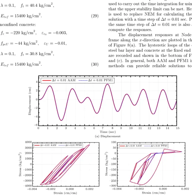
The displacement responses at Node 2 of the frame along the x-direction are plotted in the top plot of Figure 8(a). The hysteretic loops of the outermost steel bar layer and concrete at the xed end of column are recorded and shown in the bottom of Figure 8(b) and (c). In general, both AAM and PFM1 integration methods can provide reliable solutions to the very
complex nonlinear problem as shown in Figure 7. The bottom plot reveals that the material experiences a nonlinear behavior during the vibration for both concrete and steel. It is clearly indicated by this example that PFM can have unconditional stability since the highest frequency mode is as large as 9:1105
rad/sec. In addition, the capability of using PFM to solve a highly nonlinear system is veried since it can result in a reliable solution without involving any iteration procedure in each time step.
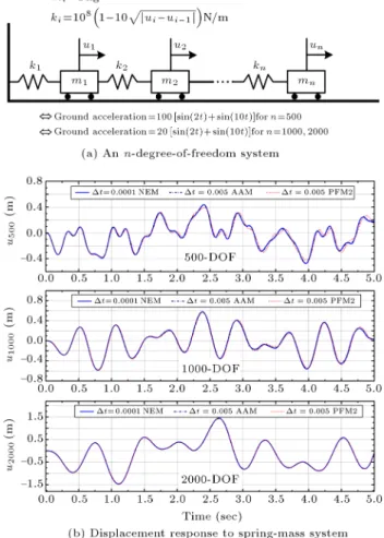
7.3. Example 3: Computational eciency In order to study the computational eciency of PFM, an n-degree-of-freedom spring mass system, as shown in Figure 9(a), is considered, where mi= 1 kg and ki=
1081 10pjui ui 1j (N/m) for i = 1; 2; 3; :::; n
are taken. Notice that ui is the displacement
corre-sponding to the ith spring mass (or the ith degree of freedom). The responses to the 500-DOF (n = 500), 1000-DOF (n = 1000), and 2000-DOF (n = 2000) systems are computed by using NEM, AAM, and PFM2. These spring-mass systems are excited by the combinations of sine loads as shown in Figure 9(a). It is found that the lowest natural frequency of the 500-DOF system is 31.38 rad/sec before it deforms, while it is 15.70 rad/sec and 7.85 rad/sec for 1000-DOF and 2000-DOF systems, respectively. On the other hand, the three systems have the same highest natural frequency equal to 20000.0 rad/sec. A time step of t = 0:0001 sec is chosen to follow the stability conditions for NEM, while the time step of t = 0:005 sec is selected for AAM and PFM2 based on accuracy consideration. The running codes are written in Fortran®, and the
execution platform is a personal computer with Intel®
CoreTM i5 CPU M460 @ 2.53 GHz with installed
memory of (RAM) 4.00 GB.
The displacement response time histories of the three systems are calculated and shown in Figure 9(b). The numerical solution obtained from NEM with a very small time step is considered as the reference solution. In general, PFM2 can have reliable solutions with com-parable accuracy to AAM. The CPU time consumed by each of the aforementioned methods in the analysis is recorded and summarized in Table 1. It is interesting to note that the CPU time consumed by PFM2 is about 10% to 20% of that consumed by NEM, and only about 2% to 3% of that consumed by AAM. This is because
Figure 9. The spring-mass systems and their responses. PFM2 can have the unconditional stability and, thus, there is no constraint on selecting an appropriate step size based on stability consideration. Notice that a very small step size is adopted for NEM since it is only conditionally stable. On the other hand, PFM2 can have an explicit formulation and, thus, it involves no nonlinear iteration for each time step and can save many computational eorts. Apparently, an iteration procedure, which is very time consuming for a matrix of a large order, is needed in each time step for AAM since AAM is an implicit method although it possesses the unconditional stability.
8. Conclusions
A new family of explicit time integration methods is proposed herein. The numerical properties of the Table 1. Comparison of CPU times.
N-DOF CPU(NEM) (1)
CPU(AAM)
(2)
CPU(PFM2)
(3) (3)/(1) (3)/(2)
500 478.48 1532.67 45.32 0.095 0.030
1000 1588.48 13567.28 302.66 0.191 0.022
proposed family method are controlled by a free pa-rameter, p. This family method is a one-step method and, thus, it is a self-starting integration method. In addition, it has unconditional stability, second-order accuracy, explicit formulation, and favorable numerical dissipation. The value of p ranges from 0 to 1. As the p value is close to 1, it leads to low numerical damping for high-frequency modes and a zero numerical damping ratio can be achieved for p = 1. On the other hand, as the p value is close to 0, it results in high numerical damping for high-frequency modes and, thus, the spurious participation of high-frequency modes can be suppressed or eliminated while the low-frequency modes can be accurately integrated. This free parameter, p, can be considered as an indi-cator variable of numerical damping for high-frequency modes. In addition, the range of 0:5 p 1 is highly recommended for practical application since the range of 0 < p < 0:5 may result in too much period distortion and numerical dissipation for the low-frequency modes. The computational eciency of this family method is evident from the numerical experiments when com-pared to the conventional integration methods. This is mainly because it can integrate the unconditional stability with explicit formulation.
Acknowledgment
The authors acknowledge the nancial support of this study by the National Science Council, Taiwan, R.O.C., under Grant No. NSC-100-2221-E-027-062. References
1. Houbolt, J. \A recurrence matrix solution for the dynamic response of elastic aircraft", Journal of Aero-nautical Science, 17, pp. 540-550 (1950).
2. Newmark, N. \A method of computation for structural dynamics", Journal of Engineering Mechanics Divi-sion, ASCE, 85, pp. 67-94 (1959).
3. Wilson, E., Farhoomand, I. and Bathe, K.J. \Nonlin-ear dynamic analysis of complex structures", Earth-quake Engineering and Structural Dynamics, 1, pp. 241-252 (1973).
4. Hilber, H., Hughes, T.J.R. and Taylor, R. \Improved numerical dissipation for time integration algorithms in structural dynamics", Earthquake Engineering and Structural Dynamics, 5, pp. 283-292 (1977).
5. Wood, W., Bossak, M. and Zienkiewicz, O.C. \An alpha modication of Newmark's method", Interna-tional Journal for Numerical Methods in Engineering, 15, pp. 1562-1566 (1980).
6. Chung, J. and Hulbert, G. \A time integration algo-rithm for structural dynamics with improved numerical dissipation: The generalized- method", Journal of Applied Mechanics, 60(6), pp. 371-375 (1993).
7. Bathe, K.J. and Baig, M.M. \On a composite implicit time integration procedure for nonlinear dynamics", Computers & Structures, 83(31-32), pp. 2513-2524 (2005).
8. Zhou, X. and Tamma, K.K. \Design, analysis, and synthesis of generalized single step single solve and optimal algorithms for structural dynamics", Interna-tional Journal for Numerical Method in Engineering, 59, pp. 597-668 (2004).
9. Zhou, X. and Tamma, K.K. \Algorithms by design with illustrations to solid and structural mechan-ics/dynamics", International Journal for Numerical Methods in Engineering, 66, pp. 1738-1790 (2006).
10. Rezaiee-Pajand, M. and Alamatian, J. \Numerical time integration for dynamic analysis using a new higher order predictor-corrector method", Engineering Computations, 25(6), pp. 541-568 (2008).
11. Gholampour, A.A. and Ghassemieh, M. \Nonlinear structural dynamics analysis using weighted residual integration", Mechanics of Advanced Materials and Structures, 20(3), pp. 199-216 (2013).
12. Shojaee, S., Rostami, S. and Abbasi, A. \An uncon-ditionally stable implicit time integration algorithm: Modied quartic B-spline method", Computers & Structures, 153, pp. 98-111 (2015).
13. Rostami, S., Shojaee, S. and Saari, H. \An explicit time integration method for structural dynamics using cubic B-spline polynomial functions", Scientia Iranica, 20(1), pp. 23-33 (2013).
14. Rezaiee-Pajand, M. and Karimi-Rad, M. \A new explicit time integration scheme for nonlinear dynamic analysis", International Journal of Structural Stability and Dynamics, 16(9), 1550054 (26 pages) (2015).
15. Chang, S.Y. \Explicit pseudodynamic algorithm with unconditional stability", Journal of Engineering Me-chanics, ASCE, 128(9), pp. 935-947 (2002).
16. Chang, S.Y. \Improved explicit method for structural dynamics", Journal of Engineering Mechanics, ASCE, 133(7), pp. 748-760 (2007).
17. Chang, S.Y. \An explicit method with improved sta-bility property", International Journal for Numerical Method in Engineering, 77(8), pp. 1100-1120 (2009).
18. Chang, S.Y. \A new family of explicit method for linear structural dynamics", Computers & Structures, 88(11-12), pp. 755-772 (2010).
19. Chang, S.Y. \Family of structure-dependent explicit methods for structural dynamics", Journal of En-gineering Mechanics, 140(6), 06014005 (7 pages) (2014a).
20. Chang, S.Y. \A family of non-iterative integration methods with desired numerical dissipation", Interna-tional Journal of Numerical Methods in Engineering,
100, pp. 62-86 (2014b).
21. Chang, S.Y. \A general technique to improve sta-bility property for a structure-dependent integration method", International Journal for Numerical Meth-ods in Engineering, 101(9), pp. 653-669 (2014c).
22. Chang, S.Y. \Comparisons of structure-dependent explicit methods for time integration", International Journal of Structural Stability and Dynamics, 15(3), 1450055 (20 pages) (2015a).
23. Chang, S.Y. \Dissipative, non-iterative integration algorithms with unconditional stability for mildly nonlinear structural dynamics", Nonlinear Dynamics, 79(2), pp. 1625-1649 (2015b).
24. Lax, P. and Richmyer, R. \Survey of the stability of linear dierence equations", Communications on Pure and Applied Mathematics, 9, pp. 267-293 (1956).
25. Lambert, J.D., Computational Method in Ordinary Dierential Equations, London: John Wiley (1973).
26. Belytschko, T. and Hughes, T.J.R. Computational Methods for Transient Analysis, North-Holland: El-sevier Science Publishers B.V. (1983).
27. Bathe, K.J., Finite Element Procedure in Engineering Analysis, Englewood Clis, NJ, USA.: Prentice-Hall, Inc. (1986).
28. Hughes, T.J.R., The Finite Element Method, Toronto, Canada: General Publishing Company Ltd. (1987).
29. Zienkiewicz, O.C., The Finite Element Method, Lon-don: McGraw-Hill (1977).
30. Goudreau, G. and Taylor, R. \Evaluation of numerical methods in elastodynamics", Journal of Computer Methods in Applied Mechanics and Engineering, 2, pp. 69-73 (1973).
31. Hilber, H. and Hughes, T.J.R. \Collocation, dissi-pation, and `overshoot' for time integration schemes in structural dynamics", Earthquake Engineering and Structural Dynamics, 6, pp. 99-118 (1978).
32. Yassin, M.H.M. \Nonlinear analysis of prestressed con-crete structures under monotonic and cycling loads", PhD Dissertation, University of California, Berkeley, California (1994).
33. Filippou, F.C., Popov, E.P. and Bertero, V.V. Ef-fects of Bond Deterioration on Hysteretic Behavior of Reinforced Concrete Joints, Earthquake Engineering Research Center, University of California, Berkeley, California (1983).
Biographies
Shuenn-Yih Chang received a PhD degree from the University of Illinois, Urbana-Champaign, in 1995. He currently serves as a distinguished professor at the
National Taipei University of Technology. His research focuses on the structural dynamics and earthquake engineering. His work addresses dynamic testing of large-scale earthquake resistant structures, including the development of novel pseudo-dynamic techniques. He is also greatly interested in the design of accurate and ecient computational methods for dynamic prob-lems of contemporary engineering. He has published more than one hundred refereed journal articles since 1988.
Ngoc-Cuong Tran received his BS and MS degrees from the Department of Civil Engineering at Hanoi Ar-chitectural University, Vietnam. He was awarded the Taiwan Government Scholarship for his PhD course. He received the PhD degree from the Department of Civil Engineering at the National Taipei University of Technology in 2016. His research interests are in the areas of structural analysis, structural dynamics, and nonlinear time-history analysis.
Tsui-Huang Wu received his BS degree from the Department of Civil Engineering at National Central University in 1979, his MS degree from the Civil En-gineering Department at National Taiwan University in 1983, and his PhD from the Banking and Finance Department at Tamkang University in 2013. Currently, he is studying a PhD course in the Department of Civil Engineering at National Taipei University of Technology. His research interests are in the areas of designing and investigation of buildings damaged by re, designing and safety assessment for civil and structural engineering in high-rise buildings, soil and structure interaction under earthquake loading, and structural analysis.
Yuan-Sen Yang is an Associate Professor at the National Taipei University of Technology. He also serves as a Committee Chairman of Information Com-mittee of the Chinese Society of Structural Engineering in Taiwan. Before serving in university, he was a Research Associate in the National Center for Research on Earthquake Engineering. He received BS from National Chung-Hsing University in 1995 and PhD from National Taiwan University in 2000. His research interests center on image analysis of structural experi-ments, high-performance computing of nonlinear nite element analysis, and numerical modeling of nonlinear structural dynamics. His teaching includes computer programming, numerical analysis, engineering statis-tics, engineering materials, structural experiments, parallel computing, and scientic visualization.