ISSN: 2322-1666 print/2251-8436 online
A FOURTH-ORDER ITERATIVE METHOD FOR COMPUTING THE MOORE-PENROSE INVERSE HAMID ESMAEILI∗, RAZIYEH ERFANIFAR AND MAHDIS RASHIDI
Abstract. In this study, a new fourth-order method to compute the Moore-Penrose inverse is proposed. Convergence analysis along with the error estimates of the method is investigated. Every itera-tion of the method involves four matrix multiplicaitera-tions. A wide set of numerical comparisons of the proposed method with nine higher order methods shows that the average number of matrix multipli-cations and the average CPU time of our method are considerably less than those of other methods.
Key Words: Moore-Penrose inverse; Iterative method; Schulz-type method; Fourth-order convergence; Matrix multiplication.
2010 Mathematics Subject Classification:Primary: 15A09; Secondary: 65F30, 65G50.
1. Introduction
Many higher order iterative methods have been developed to compute the Moore-Penrose inverse of a matrix. Iterative algorithms are a subject of current research (see, e.g., [10,11,17,21,24]), due to the importance of the topic in engineering and applied problems such as linear equations, statistical regression analysis, filtering, signal and image processing, and control of robot manipulators [5,9,14,16].
In this article, we focus on presenting and demonstrating a new method as fast as possible with a close attention to reducing the computational time. To this end, we investigate a convergent iterative method to find the Moore-Penrose inverse, which could be viewed as an extension of
Received: 1 July 2016, Accepted: 02 February 2017. Communicated by Ali Taghavi; ∗Address correspondence to H. Esmaeili; Email: [email protected].
c
2017 University of Mohaghegh Ardabili. 52
the famous Schulz method for such a purpose. It is proved that this method always converges with fourth-order, and every iteration involves four matrix multiplications. A theoretical discussion will also be given to show the behavior of proposed scheme.
In the simple case, when A is a n×n nonsingular complex matrix, to compute the matrix inverse, various iterative methods, called Schulz-type methods, already developed [1, 4, 7, 10, 12, 15, 18, 20, 23, 24], almost all of which are based on iterative solvers for the scalar equation
f(x) = 1x−a= 0 applied to the matrix equation
f(X) =X−1−A= 0.
We should also point out that even if the matrix A is singular, these methods converge to the Moore-Penrose inverse using a proper initial matrix. A full discussion on this feature of this type of iterative methods has been given in [1,2]. So, upon this observation, we first assume that matrixA is an×nnonsingular matrix.
The rest of this paper is organized as follows. Section 2 is devoted to presenting some existing iterative schemes to find matrix inverse. Also, we propose our new method in Section 2 and prove that it is fourth-order convergent. In Section 3, we show that one can use our method to find the Moore-Penrose inverse. In Section 4, some numerical examples are given to show the performance of the presented method compared with nine higher order methods. Finally, some conclusions are outlined in Section 5.
2. Schulz-type iterative methods
Suppose that A is a n×n nonsingular complex matrix. There are various iterative methods, called Schulz-type methods, to computeA−1. In the sequel, we remind some of them.
Perhaps, the most frequently used iterative method to approximate
A−1 is the famous Newton method
(2.1) Xk+1 =Xk(2I−AXk), k= 0,1,2, . . . ,
originated in [15], in which I is the identity matrix with the same di-mension as that of matrixA. Note that each iteration of (2.1) involves two matrix multiplications. Schulz in [15] found that the eigenval-ues of I −AX0 must have magnitudes less than 1 to ensure the
con-vergence. Since the residuals Ek = I −AXk in each step (2.1) sat-isfy kEk+1k ≤ kAk kEkk2, Newton method is a second-order iterative
method [1]. Similarly, in [10] the relation kAεk+1k ≤ kAεkk2 is verified
for errors of the formεk =Xk−A−1.
Li et al. in [8] investigated the following third-order method, known as Chebyshev method,
(2.2) Xk+1=Xk(3I−AXk(3I−AXk)),
and also proposed another iterative method to find A−1 of the same order as given in
(2.3) Xk+1=Xk(I+ 0.5(I−AXk)(I + (2I −AXk)2)).
We observe that each iteration of (2.2) and (2.3) contain 3 and 4 matrix multiplications, respectively. Toutounian and Soleymani [23] proposed the following fourth-order method that involves 5 matrix multiplications: (2.4) Xk+1= 0.5Xk(9I−AXk(16I−AXk(14I−AXk(6I−AXk))))).
Krishnamurthy and Sen [6] provided the following fourth-order method that contains 4 matrix multiplications:
(2.5) Yk=I−AXk,
Xk+1=Xk(I+Yk(I+Yk(I+Yk))).
As another example, a ninth-order method, could be presented as
Xk+1 =Xk(I+Yk(I+Yk(I+Yk(I+Yk(I+Yk(I+Yk(I+Yk(I+Yk)))))))).
The number of matrix multiplications of the above method can be re-duced from 9 to 7 if it is rewritten as follows:
(2.6)
Bk=Yk2, Ck=Bk2, Dk=Ck2,
Xk+1=Xk((I+Yk)(I +Bk)(I+Ck) +Dk).
Soleymani et al. [19] provided the following sixth-order method that contains 5 matrix multiplications:
(2.7)
Bk=AXk
Sk=Bk(−I +Bk)
Soleymani and Stanimirovi´c [18] investigated the following ninth-order method that has 7 matrix multiplications in each iteration:
(2.8)
Bk=AXk
Sk=−7I+Bk(9I+Bk(−5I+Bk)) Tk=BkSk
Xk+1=−0.125XkSk(12I+Tk(6I+Tk)).
Also, Soleymani et al. [20] proposed another ninth-order method, again involving 7 matrix multiplications in each iteration, as
(2.9)
Bk=AXk
Sk= 3I+Bk(−3I+Bk) Tk=BkSk
Xk+1=−19XkSk(−29I+Tk(33I+Tk(−15I + 2Tk))).
Remark 2.1. All of the above methods are initiated by (2.10) X0 =αA∗, 0< α <
2
σ12,
in which σ1 denote the largest singular value of A. There are another
choices for X0 too. A discussion on choosing the initial approximation
X0 is given in [2, 11]. Perhaps, in general case, the simplest choice for X0 is
(2.11) X0 =αA∗,
in which α is an appropriate constant.
Beside the above methods, we investigate our method to find Moore-Penrose inverse as follows:
Xk+1=Xk
9I−26(AXk) + 34(AXk)2−21(AXk)3+ 5(AXk)4
.
We can rewrite our method in the way
(2.12)
Bk=AXk Ck=Bk2
Xk+1=Xk[9I−26Bk+Ck(34I−21Bk+ 5Ck)].
Note that every iteration of the method (2.12) involves four matrix mul-tiplications. In the sequel, we prove that the method (2.12) is fourth-order convergent.
Let us consider the following singular value decomposition of the ma-trixA:
(2.13) A=U SV∗, S =diag(σ1, . . . , σn), σ1≥ · · · ≥σn>0,
whereU and V are unitary matrices. Using (2.14) X0 =βA∗,
in whichβ is a constant, we can deduce that each iterate of the method (2.12) has a singular value decomposition of the form
Xk=V SkU∗, Sk=diag(s (k) 1 , . . . , s
(k) n ),
where
S0=βS,
and
(2.15) Sk+1=Sk9I−26SSk+ 34(SSk)2−21(SSk)3+ 5(SSk)4.
Therefore, the diagonal matricesRk=SSk=diag(r (k) 1 , . . . , r
(k)
n ) satisfy Rk+1:=g(Rk) = 9Rk−26Rk2 + 34R3k−21R4k+ 5R5k,
that means
(2.16) r(k+1)i =g(ri(k)) = 9r(k)i −26r(k)2i + 34r(k)3i −21r(k)4i + 5r(k)5i .
In the following theorem, we show that the sequences (2.16) are fourth-order convergent to ri = 1 for any r(0)i ∈ (0,1 +γ), in which γ is a suitable constant.
Theorem 2.2. For any initial point r(0) ∈ (0,1 + γ), the sequence r(k+1) =g(r(k)) is fourth-order convergent to r = 1, in which the func-tiong(r) is defined by (2.16) and γ = 0.53.
Proof. We can find that the real fixed points and the critical points of
g(r) as follows:
g(r) =r =⇒ r= 0, 1, 1 +γ, g0(r) = 0 =⇒ r= 0.36, 1, 1, 1,
in which
γ = 1 15
"
1 + 3
q
316 + 30 √
114− 14
3 p
316 + 30√114
#
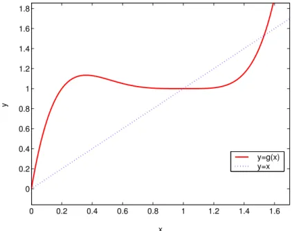
Notingg00(0.36) =−6.55 <0 and g(4)(1) = 96>0, we can deduce that 0.36 is a local maximizer and 1 is a local minimizer of g(r). On the other hand,g(0) = 0<1 =g(1) andg(0.36)≈1.13<1 +γ =g(1 +γ). Therefore, r = 0,1 and r = 0.36,1 +γ are minimizer and maximizer of g(r) in the interval [0,1 +γ], respectively. Moreover, the interval [0,1 +γ] maps into itself by the functiong(r).
0 0.2 0.4 0.6 0.8 1 1.2 1.4 1.6 0
0.2 0.4 0.6 0.8 1 1.2 1.4 1.6 1.8
x
y
y=g(x) y=x
Figure 1. Graphs of the liney=xand the functiony=g(x).
Considering an arbitrary initial pointr(0) ∈(0,1 +γ), one can easily obtain the following considerations (For clarification, see Figure1):
• The unique solution of the equationg(r) = 1 in the interval [0,1) is 15.
• g(r) is increasing in the interval (0,15). Therefore, ifr(k)∈(0,15), for some k, then there exists an index k0 ≥ k such that either
r(k0)= 15, and so r(k0+1) = 1, orr(k0+1)∈(15,1). • Ifr(k)∈(15,1), for some k, thenr(k+1)∈(1,1 +γ).
• Ifr(k) ∈(1,1 +γ), for some k, then the sequence {r(k+`)}`≥1 ⊆
Noting the above considerations, we can conclude that the sequence
r(k+1) =g(r(k)) is convergent tor = 1. On the other hand,
g0(1) =g00(1) =g000(1) = 0
implies that the convergence is fourth-order (See [3]).
Considering Theorem 2.2, we conclude that if βσ12 =r1(0) ∈(0,1.53), thenβσi2 =ri(0)∈(0,1.53), for all i, and
lim
k→∞Rk=I.
Hence,
lim
k→∞Sk=S −1,
so
lim
k→∞Xk=V S
−1U∗ =A−1.
Moreover, the order of convergence is four. Therefore, the following theorem is proved.
Theorem 2.3. Consider the nonsingular matrix A, and suppose that σ21 denotes the largest singular value of A. Moreover, assume that the initial approximationX0 is defined by (2.14), in which
(2.17) 0< β < 1.53 σ2
1 .
Then, the sequence{Xk}k≥0 generated by (2.12) converges to the inverse matrixA−1 with fourth-order.
Remark 2.4. Consider the initial matrix X0 according to (2.14), with
β from (2.17). Sinceσ21 is a (the) largest singular value of A, we have
σ21 =kAk2
2 ≤ kAk1kAk∞. Therefore, the selection
(2.18) β= 1
kAk1kAk∞
3. Moore-Penrose inverse
The Moore-Penrose inverse of am×ncomplex matrixA, denoted by
A†, is a unique n×m matrix X satisfying the following four Penrose equations:
(3.1) AXA=A, XAX =X, (AX)∗=AX, (XA)∗ =XA,
whereA∗ is the conjugate transpose of A.
Now, suppose that rank(A) = r ≤ min{m, n} and consider the sin-gular value decomposition of Aas follows:
A=U
S 0 0 0
V∗, S =diag(σ1, . . . , σr), σ1≥ · · · ≥σr>0.
It is well known that
A†=V
S−1 0
0 0
U∗.
Let us now extend the contributed method (2.12) for calculating the Moore-Penrose inverseA†. That is, we must analytically reveal that the sequence{Xk}k≥0 generated by the iterative Schulz-type method (2.12),
tends to the Moore-Penrose inverse as well.
Using mathematical induction, it would be easy to check that the iterates produced at each cycle of (2.12) satisfy the following relations: (3.2) (AXk)
∗=AX
k, (XkA)∗ =XkA, A†AXk=Xk, XkAA†=Xk.
If we take X0=βA∗, which β is defined by (2.17), then X0 =αA∗=V
S0 0
0 0
U∗,
where
S0 =βS.
is a diagonal matrix. Therefore,
V∗X0U =
S0 0
0 0
.
Now, the principle of mathematical induction and (3.2) lead to
(3.3) V∗XkU =
Sk 0
0 0
,
in whichSk is a diagonal matrix satisfying the following relation: (3.4) Sk+1=Sk
9I−26SSk+ 34(SSk)2−21(SSk)3+ 5(SSk)4
.
This is the same as (2.15) and the proof of the Theorem 2.2show that lim
k→∞Sk=S −1.
Therefore,
lim
k→∞Xk=V
S−1 0 0 0
U∗ =A†.
Moreover, the order of convergence is four. Hence, we have the following theorem.
Theorem 3.1. Let A be am×ncomplex matrix of rankr and suppose that σ1 is the largest singular value of A. Moreover, assume that the initial approximation X0 is defined by (2.14), in which β is defined by (2.17). Then, the sequence {Xk}k≥0 generated by (2.12) converges to the Moore-Penrose inverseA† with fourth-order.
Remark 3.2. Ifm≤n, then we apply (2.12) in the same form, in which
Idenotes them×midentity matrix. On the other hand, for casem > n
we must apply (2.12) with A∗ instead of A and use the n×n identity matrix. So, for the casem > n, we compute (A∗)†, that is (A†)∗.
We can study the convergence properties of the algorithm (2.12) using the error matrixEk=Xk−A†. The matrix formula representingEk+1is
a sum of possible zero-order term consisting of a matrix which does not depend uponEk, one or more first-order matrix terms in which Ek or Ek∗ appears only once, one or more second-order terms in whichEkand Ek∗ appear at least twice, and so on [13]. To compute error estimates, first note that
A†AEk=Ek, EkAA†=Ek
according to (3.2). Therefore,
Xk(AXk) =A†+ 2Ek+EkAEk,
Xk(AXk)2=A†+ 3Ek+ 3EkAEk+ (EkA)2Ek,
Xk(AXk)3=A†+ 4Ek+ 6EkAEk+ 4(EkA)2Ek+ (EkA)3Ek, Xk(AXk)4=A†+ 5Ek+ 10EkAEk+ 10(EkA)2Ek+ 5(EkA)3Ek
Now, substituting Xk=A†+Ek in (2.12) results in
A†+Ek+1=Xk+1
= 9Xk−26XkAXk+ 34Xk(AXk)2−21Xk(AXk)3
+ 5Xk(AXk)4
=A†+ 7(EkA)3Ek+ 8(EkA)4Ek,
such that
(3.5) Ek+1 = 7(EkA)3Ek+ 8(EkA)4Ek.
Hence, we have the following theorem.
Theorem 3.3. Let A be am×nnonzero complex matrix. If the initial approximation X0 is defined by (2.14), with β from (2.17), then
kA(X0−A†)k<1,
and iterative method (2.12) converges to A† with fourth-order. Its first, second, third, fourth and fifth order error terms are given by
(3.6)
error1 =error2=error3 = 0, error4 = 7(EkA)3Ek,
error5 = 8(EkA)4Ek.
in which Ek =Xk−A† denotes the error matrix.
Proof. Take P =AA† andS =I−AX0. Then,P2 =P and P S=AA†(I−AX0) =AA†−AX0
=AA†−AX0AA†= (I−AX0)AA†=SP.
On the other hand, it is proved [22] that for n×n matrices M and N
such that M2 =M and M N =N M, one has
ρ(M N)≤ρ(N).
Consequently, we attain
ρ(A(X0−A†)) =ρ(A(βA∗−A†))
≤ρ(I−βAA∗) = max
1≤i≤r|1−λi(βAA ∗)|
= max
1≤i≤r|1−βσ 2 i|.
By using (2.17), we conclude that
kAE0k=kA(X0−A†)k ≤ρ(A(X0−A†))≤ max
1≤i≤r|1−βσ 2 i|<1.
Now, we can immediately derive (3.6) from (3.5). Furthermore, (3.5) results in
AEk+1 = 7(AEk)4+ 8(AEkA)5.
Hence,
kAEk+1k ≤(7 + 8kAEkk)kAEkk4,
and thereforekAEkk →0, sincekAE0k<1. On the other hand,
kEk+1k=kA†AEk+1k ≤ kA†k kAEk+1k ≤ kA†k(7 + 8kAEkk)kAEkk4
results in
kEk+1k ≤ h
kA†k kAk4(7 + 8kAk kEkk) i
kEkk4.
Consequently,Xk→A† and the order of convergence is four.
4. Numerical experiments
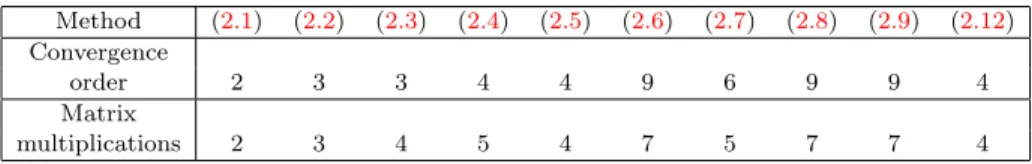
In this section, we will make some numerical comparisons of our pro-posed method (2.12) with other methods presented here. To this end, we focus on the total number of matrix multiplications and CPU times required for convergence. Table 1 denotes convergence order and number of matrix multiplications in any iteration of different methods.
Table 1. Convergence order and number of matrix multiplications for different methods Method (2.1) (2.2) (2.3) (2.4) (2.5) (2.6) (2.7) (2.8) (2.9) (2.12) Convergence
order 2 3 3 4 4 9 6 9 9 4
Matrix
multiplications 2 3 4 5 4 7 5 7 7 4
We present three different types of tests. Test 1 is devoted to compar-ing the schemes to find the inverse of some randomly generated dense square matrices, Test 2 gives some comparison to find the Moore-Penrose inverse of dense matrices, and Test 3 gives some comparison to find the Moore-Penrose inverse of some randomly generated large sparse matri-ces. All tests were carried out with a Matlab code while the computer specifications are Microsoft Windows XP Intel(R), Pentium(R) 4, CPU
2.60 GHz, with 2 GB of RAM. We use the initial matrix X0 defined in (2.14), withβ from (2.17). The stop criterion is
kXk+1−Xkk∞
1 +kXkk∞
<10−7
and the maximum number of iterations is set to 100 in our written codes as the maximum number of cycle for the methods is considered in comparisons.
Test 1. In this test, we compute the inverse of dense nonsingular square matrixA, where 10 matrices of the sizesm×m,m= 100,200,300,400,500, are randomly generated as follows:
A= 100rand(m, m)−10rand(m, m).
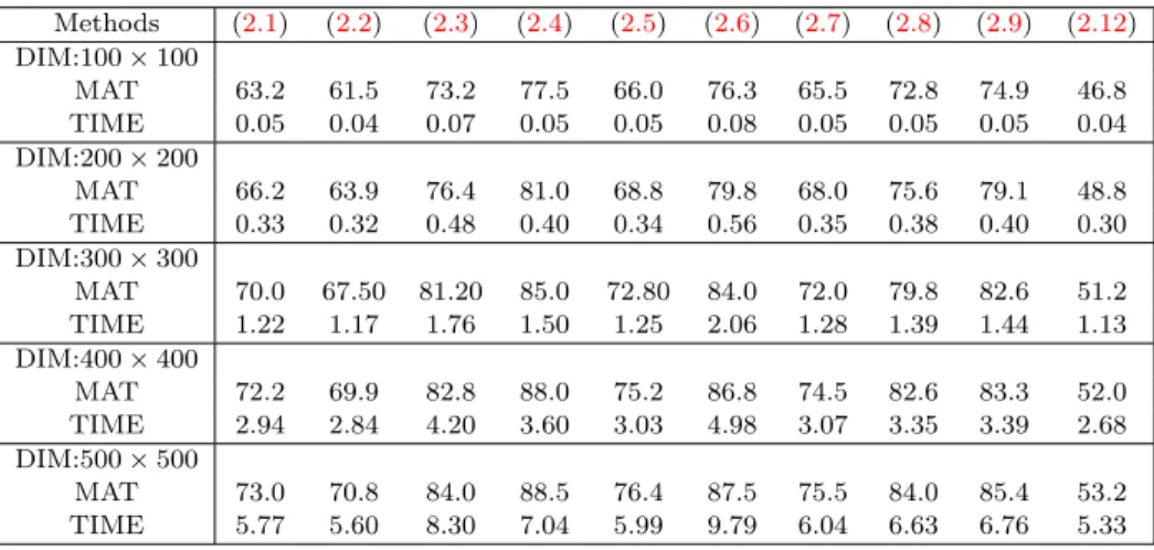
Average number of matrix multiplications and average of CPU times required for convergence are listed in Table 2. In this table, DIM, MAT and TIME denote the size ofA, average values of matrix multiplications and elapsed times in seconds, respectively.
Table 2. Average values of matrix multiplications and elapsed times to compute the inverse of a dense nonsingular square matrix by different methods
Methods (2.1) (2.2) (2.3) (2.4) (2.5) (2.6) (2.7) (2.8) (2.9) (2.12) DIM:100×100
MAT 63.2 61.5 73.2 77.5 66.0 76.3 65.5 72.8 74.9 46.8 TIME 0.05 0.04 0.07 0.05 0.05 0.08 0.05 0.05 0.05 0.04 DIM:200×200
MAT 66.2 63.9 76.4 81.0 68.8 79.8 68.0 75.6 79.1 48.8 TIME 0.33 0.32 0.48 0.40 0.34 0.56 0.35 0.38 0.40 0.30 DIM:300×300
MAT 70.0 67.50 81.20 85.0 72.80 84.0 72.0 79.8 82.6 51.2 TIME 1.22 1.17 1.76 1.50 1.25 2.06 1.28 1.39 1.44 1.13 DIM:400×400
MAT 72.2 69.9 82.8 88.0 75.2 86.8 74.5 82.6 83.3 52.0 TIME 2.94 2.84 4.20 3.60 3.03 4.98 3.07 3.35 3.39 2.68 DIM:500×500
MAT 73.0 70.8 84.0 88.5 76.4 87.5 75.5 84.0 85.4 53.2 TIME 5.77 5.60 8.30 7.04 5.99 9.79 6.04 6.63 6.76 5.33
From Table 2, we can see that our method (2.12) is more better than others both in matrix multiplications and CPU time. The worst one is fourth-order method (2.4). Note that the ninth-order method (2.8) acts like the third-order method (2.3). [Also, the sixth-order method (2.7) acts like the fourth-order method (2.5)]. The third-order method (2.2) and the second-order method (2.1) are better than other higher order
methods, although they are not comparable with our method (2.12). Hence, we can consider the scheme (2.12) as the fastest method.
Test 2. In this test, we compute the Moore-Penrose inverse of randomly generated dense matrixA of the size m×n,n=m+ 50, as follows:
A= 100rand(m, n)−10rand(m, n).
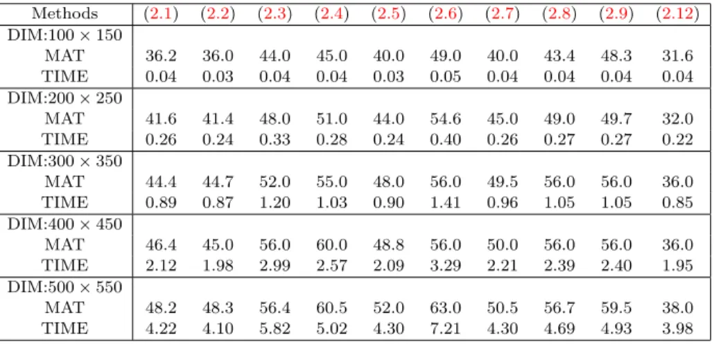
Again, for each m= 100,200,300,400,500, we have performed 10 tests and compared the average values of matrix multiplications and elapsed times in seconds. The results of comparisons are reported in Table 3, in terms of the number of matrix multiplications and the computational time (in seconds).
From Table 3, we can see that our method (2.12) is more better than others both in matrix multiplications and CPU time. The worst one is ninth-order method (2.6). Note that the ninth-order method (2.8) acts like the third-order method (2.3). [Also, the sixth-order method (2.7) acts like the fourth-order method (2.5)]. The third-order method (2.2) and the second-order method (2.1) are better than other higher order methods, although they are not comparable with our method (2.12). Hence, we can consider the scheme (2.12) as the fastest method.
Table 3. Average values of matrix multiplications and elapsed times to compute the Moore-Penrose inverse of a dense rectangular matrix by different methods Methods (2.1) (2.2) (2.3) (2.4) (2.5) (2.6) (2.7) (2.8) (2.9) (2.12) DIM:100×150
MAT 36.2 36.0 44.0 45.0 40.0 49.0 40.0 43.4 48.3 31.6 TIME 0.04 0.03 0.04 0.04 0.03 0.05 0.04 0.04 0.04 0.04 DIM:200×250
MAT 41.6 41.4 48.0 51.0 44.0 54.6 45.0 49.0 49.7 32.0 TIME 0.26 0.24 0.33 0.28 0.24 0.40 0.26 0.27 0.27 0.22 DIM:300×350
MAT 44.4 44.7 52.0 55.0 48.0 56.0 49.5 56.0 56.0 36.0 TIME 0.89 0.87 1.20 1.03 0.90 1.41 0.96 1.05 1.05 0.85 DIM:400×450
MAT 46.4 45.0 56.0 60.0 48.8 56.0 50.0 56.0 56.0 36.0 TIME 2.12 1.98 2.99 2.57 2.09 3.29 2.21 2.39 2.40 1.95 DIM:500×550
MAT 48.2 48.3 56.4 60.5 52.0 63.0 50.5 56.7 59.5 38.0 TIME 4.22 4.10 5.82 5.02 4.30 7.21 4.30 4.69 4.93 3.98
Test 3. This experiment evaluates the applicability of the new method (2.12) to find Moore-Penrose inverse of 10 random large sparse matrices of the size 1000×1500 containing approximately 6000 nonzero entries
as follows:
A=sprand(1000,1500,0.004).
The results of comparisons are reported in Table 4, in terms of number of matrix multiplications and computational time (in seconds).
Table 4. Average values of matrix multiplications and elapsed times to compute the Moore-Penrose inverse of a 1000×1500 matrix by different methods
Methods (2.1) (2.2) (2.3) (2.4) (2.5) (2.6) (2.7) (2.8) (2.9) (2.12) MAT 47.4 46.5 56.0 58.5 50.8 60.9 50.5 55.3 58.8 36.8 TIME 85.35 91.38 115.64 120.01 103.33 129.42 113.30 123.83 133.64 74.36
From Table 4, we can see that our method (2.12) is more better than others both in matrix multiplications and CPU time. The worst one is ninth-order method (2.6). Note that the ninth-order method (2.8) acts like the third-order method (2.3). [Also, the sixth-order method (2.7) acts like the fourth-order method (2.5)]. The third-order method (2.2) and the second-order method (2.1) are better than other higher order methods, although they are not comparable with our method (2.12). Hence, we can consider the scheme (2.12) as the fastest method.
5. Conclusions
In this paper, we proposed a new method to find the Moore-Penrose inverse. It is proved that this method is fourth-order convergent. A wide set of random numerical experiments showed that its number of matrix multiplications and CPU time are considerably less than those of other higher methods. So, our method could be considered as a fast method.
Acknowledgments
The authors would like to thank the referees for their useful comments and constructive suggestions which substantially improved the quality of this paper.
References
[1] A. Ben-Israel, D. Cohen, On iterative computation of generalized inverses and associated projections, SlAM J. Numer. Anal.3(1966), 410–419.
[2] A. Ben-Israel, T.N.E. Greville, Generalized Inverses, Second ed., New York: Springer (2003).
[3] R.L. Burden, J.D. Faires, Numerical Analysis, 9th Ed. Brooks/Cole, Cengage Learning, Boston (2011).
[4] H. Chen, Y. Wang, A family of higher-order convergent iterative methods for computing the Moore-Penrose inverse, Appl. Math. Comput.218(2011), 4012– 4016.
[5] A. Cichocki, B. Unbehauen, Neural networks for optimization and signal pro-cessing, New York: John Wiley & Sons (1993).
[6] E.V. Krishnamurthy, S.K. Sen,Numerical Algorithms: Computations in Science and Engineering, New Delhi, India: Affiliated East-West Press (1986).
[7] W. Li, Z. Li, A family of iterative methods for computing the approximate in-verse of a square matrix and inner inin-verse of a non-square matrix, Appl. Math. Comput.215(2010), 3433–3442.
[8] H. B. Li, T.Z. Huang, Y. Zhang, X.P. Liu, T.X. Gu,Chebyshev-type methods and preconditioning techniques, Appl. Math. Comput.218(2001), 260–270.
[9] S. Miljkovi´c, M. Miladinovi´c, P., Stanimirovi´c, I. Stojanovi´c, Application of the pseudo-inverse computation in reconstruction of blurred images, Filomat26 (2012), 453–465.
[10] H.S. Najafi, M.S. Solary,Computational algorithms for computing the inverse of a square matrix, quasi-inverse of a non-square matrix and block matrices, Appl. Math. Comput.183(2006), 539–550.
[11] V.Y. Pan, R. Schreiber,An improved Newton iteration for the generalized inverse of a matrix with applications, SIAM J. Sci. Stat. Comput.12(1991), 1109–1131. [12] V.Y. Pan,Newton’s iteration for matrix inversion, advances and extensions, ma-trix methods: theory algorithms and applications, Singapore: World Scientific (2010).
[13] W.H. Pierce, A self-correcting matrix iteration for the Moore-Penrose inverse, Linear Algebra Appl.244(1996), 357-363.
[14] P. Roland, P.G. Beim,Inverse problems in neural field theory, SIAM J. Appl. Dynam. Sys.8(2009), 1405–1433.
[15] G. Schulz,Iterative Berechmmg der reziproken Matrix, Z. Angew. Math. Mech. 13(1933), 57–59.
[16] L. Sciavicco, B. Siciliano,Modelling and control of robot manipulators, London: Springer–Verlag (2000).
[17] X. Sheng, G. Chen: The generalized weighted Moore-Penrose inverse, J. Appl. Math. Comput.25(2007), 407–413.
[18] F. Soleymani, P.S. Stanimirovi´c,A Higher Order Iterative Method for Computing the Drazin Inverse, The Scientific World Journal Volume 2013, Article ID 708647, 11 pages, http://dx.doi.org/10.1155/2013/708647.
[19] F. Soleymani, P.S. Stanimirovi´c, M.Z. Ullah,An accelerated iterative method for computing weighted Moore-Penrose inverse, Appl. Math. Comput. 222 (2013), 365–371.
[20] F. Soleymani, H. Salmani, M. Rasouli,Finding the Moore-Penrose inverse by a new matrix iteration, J. Appl. Math. Comput.47(2015), 33-48.
[21] S. Srivastava, D.K. Gupta, A higher order iterative method for A(2)T ,S, J. Appl. Math. Comput.46(2014), 147–168.
[22] P.S. Stanimirovi´c, D.S. Cvetkovi´c-Ili´c,Successive matrix squaring algorithm for computing outer inverses, Appl. Math. Comput.203(2008), 19–29.
[23] F. Toutounian, F. Soleymani,An iterative method for computing the approximate inverse of a square matrix and the Moore-Penrose inverse of a non-square matrix, Appl. Math. Comput.224(2013), 671–680.
[24] L. Weiguo, L. Juan, Q. Tiantian, A family of iterative methods for computing Moore-Penrose inverse of a matrix, Linear Algebra Appl.438(2013), 47-56.
H. Esmaeili
Department of Mathematics, Bu-Ali Sina University, Hamedan, Iran
Email: [email protected]
R. Erfanifar
Department of Mathematics, Bu-Ali Sina University, Hamedan, Iran
Email: [email protected]
M. Rashidi
Department of Mathematics, Bu-Ali Sina University, Hamedan, Iran