ISSN: 2322-1666 print/2251-8436 online
SUMUDU TRANSFORM ITERATION METHOD FOR FRACTIONAL DIFFUSION-WAVE EQUATIONS
K. SAYEVAND∗AND K. PICHAGHCHI
Abstract. In this article, we have implemented Sumudu trans-form iteration method as a new approximate analytical technique for solving fractional diffusion-wave equations. The fractional de-rivative is described in the Caputo sense. The solution existence, uniqueness, stability and convergence of the proposed scheme is discussed. Finally, the validity and applicability of our approach is examined with the use of a solvable model method. The results presented here are in compact and elegant expressed in term of Mittag-Leffler function which are suitable for numerical computa-tion.
Key Words: Sumudu transform, Diffusion-wave equation, Caputo fractional derivative, Mittag-Leffler function.
2010 Mathematics Subject Classification:Primary: 34A08; Secondary: 35L05.
1. Introduction
In last decades, fractional calculus have been the focus of many studies due to their frequent appearance in various applications in physics, science, engineering, economics and so on. For instance, see [4,5,9–13] and references therein. Consequently, many problems in differential equations have presented and studied in the form of fractional order derivatives in the literature. In fractional calculus, the Mittag-Leffler function, as an analogous to exponential naturally function, plays an important role. In fact, the exponential function itself is a special form
Received: 8 February 2016, Accepted: 20 February 2016. Communicated Mohammad Zareb-nia;
∗Address correspondence to Khosro Sayevand; E-mail: [email protected] c
⃝2015 University of Mohaghegh Ardabili.
of these general functions. A considerable amount of literature is ded-icated to the applications of the Mittag-Lefffer function as solutions of fractional order models [7,8]. Our results in this article are based mainly on the Mittag-Leffler function. Actually, we consider the diffusion-wave equations presented in the scope of fractional calculus in the following form:
∂αξ(x, t)
∂tα =λ
∂βξ(x, t)
∂xβ ,
(1.1)
ξ(x,0) =u(x), ∂
∂tξ(x,0) =ν(x),
(1.2)
where 0< α <2,m < β ≤m+ 1,m∈N, λ∈R. Notice that, the second initial condition is forα >1 only and the operators ∂t∂αα and ∂
β
∂xβ are the Caputo fractional derivatives defined as
∂αf(t)
∂tα = [
Itm−αf(m)(t)], m−1< α < m, m∈N, dm
dtmf(t), α=m,
(1.3)
whereItα is the Riemann-Liouville integral operator of order αdefined as
Itαf(t) =
1 Γ(α)
∫t 0
f(τ)
(t−τ)1−αdτ, α >0, t >0,
f(t), α= 0.
(1.4)
In our attempt, we have used the Sumudu transform iteration method (STIM) to obtain relatively new analytic and approximate solution for fractional diffusion-wave equations. The importance of this equation usually arises in the wave propagation in beams and modeling formation of grooves on a flat surface. Additional background and application of Eq. (1.1)-(1.2) in science, engineering and mathematics can be found in [1]. Finally, convergence and stability of the proposed approach for these types of problems will be considered.
First we recall some preliminaries and notations regarding Sumudu transform.
Definition 1.1. The Sumudu transform is defined over the set of func-tions:
(1.5) A=
{
f(t)| ∃M, τ1, τ2 >0,|f(t)|< M e
|t|
by the following formula [2] (1.6) F(u) =S[f(t);u] =
∫ ∞ 0
f(ut)e−tdt, u∈(−τ, τ).
The Sumudu transform of the Caputo fractional derivative is defined as follows [3]
(1.7) S[Dαtf(t);u] =u−αS[f(t)]−
m∑−1 k=0
u−α+kf(k)(0), m−1< α≤m,
(1.8) S
[
Dtαf(x, t);u ]
=u−αS[f(x, t)]− m∑−1
k=0
u−α+kf(k)(x,0), m−1< α≤m.
Theorem 1.2. Assuming H(u) = S[h(t)] and G(u) = S[g(t)], the Sumudu convolution theorem states that the transform of
(1.9) h(t)∗g(t) =
∫ t 0
h(t−τ)g(τ)dτ, is given by
(1.10) uH(u)G(u) =S[h(t)∗g(t)].
Proof. See [2]. □
Some fundamental further established properties of Sumudu trans-form can be found in [2].
2. Sumudu transform iteration method implementation to fractional diffusion-wave equations
Now we are ready to implement STIM for obtaining analytical and numerical solutions of Eq. (1.1)-(1.2). By taking Sumudu transform from the Eq. (1.1)-(1.2), with respect to the independent variabletand using the initial conditions, we get
(2.1) u−αξ¯(x, u)−u−αξ(x,0)−u1−α∂
∂tξ(x,0) =λ
∂βξ¯(x, u)
∂xβ .
Solving for ¯ξ(x, u), we get
(2.2) ξ¯(x, u) =ξ(x,0) +u∂
∂tξ(x,0) +λu
α∂βξ¯(x, u) ∂xβ .
By notice the following Sumudu transform pair
(2.3) t
k
Γ(k+ 1)
S
←→uk,
and by applying the inverse Sumudu transform to both sides of Eq. (2.2), and using the convolution Theorem1.2, we get
ξ(x, t) =ξ(x,0) +t∂
∂tξ(x,0) + tα−1
Γ(α) ∗λ
∂βξ¯(x, u)
∂xβ
=ξ(x,0) +t∂
∂tξ(x,0) + λ
Γ(α)
∫ t 0
(t−τ)α−1∂
βξ(x, τ) ∂xβ dτ.
(2.4)
According to [6], by imposing the initial conditions to obtain the solution of Eq. (1.1)-(1.2), we can construct an iteration formula as follows
ξ0(x, t) =ξ(x,0) +t ∂
∂tξ(x,0), (2.5)
ξj+1(x, t) =ξ0(x, t) + λ Γ(α)
∫ t
0
(t−τ)α−1∂
βξ j(x, τ)
∂xβ dτ, j= 0,1,· · ·.
(2.6)
By the above iteration each term will be determined by the previous terms and the approximation of iteration formula can be entirely evalu-ated. Consequently, the solution may be written as
(2.7) ξ(x, t) = lim
j→∞ξj(x, t).
3. Existence and uniqueness of solution
Theorem 3.1. Suppose that λ∂β∂xξ(x,t)β ∈L1(0, X)×(0, T) and the STIM is applied to Eq. (1.1)-(1.2). Then, this equation has a unique solution ξ(x, t)∈L1(0, X)×(0, T).
Proof. As before, applying the Sumudu transform with respect to time variabletfrom (1.1)-(1.2) and application of the inverse Sumudu trans-form, we have
(3.1) ξ(x, t) =ξ(x,0) +t∂
∂tξ(x,0) + λ
Γ(α)
∫ t 0
(t−τ)α−1∂
βξ(x, τ) ∂xβ dτ.
Using the rule for the Caputo fractional differentiation of the power function, we easily obtain that
(3.2) ∂
α
∂tα(t
Using (3.2), the direct substitution of the function defined by the ex-pression (3.1) in the Eq. (1.1), we have
∂α ∂tα
( λ γ(α)
∫ t 0
(t−τ)α−1∂
βξ(x, τ) ∂xβ dτ
)
(3.3) = ∂
α
∂tαI α t
( λ∂
βξ(x, t) ∂xβ
)
=λ∂
βξ(x, t) ∂xβ .
Therefore,ξ(x, t) satisfies (1.1)-(1.2) and the existence of the solution is proved. Furthermore, it follows from (3.1) thatξ(x, t)∈L1(0, X)×(0, T).
The uniqueness follows from the linearity of fractional differentiation and the properties of the Sumudu transform. Indeed, if there exist two solutions ξ(x, t) and ˆξ(x, t), then ζ(x, t) = ξ(x, t)−ξˆ(x, t) must satisfy
∂α
∂tαζ(x, t) = 0. Then, the Sumudu transform ¯ζ(x, u) = 0, and therefore
ζ(x, t) = 0 almost everywhere in the considered interval, which proves that the solution inL1(0, X)×(0, T) is unique. □
4. Convergence analysis
Theorem 4.1. Under the assumption of boundedness the initial condi-tions (1.2), The STIM to approximate the solution of Eq. (1.1)-(1.2) is convergent.
Proof. Applying the STIM method to Eq. (1.1)-(1.2), we obtain the following recursive formula
ξ0(x, t) =ξ(x,0) +t ∂
∂tξ(x,0),
(4.1)
ξj+1(x, t) =ξ0(x, t) + λ
Γ(α)
∫ t 0
(t−τ)α−1∂
βξj(x, τ) ∂xβ dτ.
(4.2)
We can write (4.1) as
(4.3) ξj+1(x, t) =ξ0(x, t) +
1 Γ(α)
∫ t 0
(t−τ)α−1K(x, τ)ξj(x, τ)dτ,
therefore
(4.4) |ξ1(x, t)−ξ0(x, t)| ≤
1 Γ(α)
∫ t 0
(t−τ)α−1|K(x, τ)| |ξ0(x, τ)|dτ.
By assumption the boundedness of initial conditions, we have (4.5) K1 =||ξ(x,0)||∞<∞, K2 =||K(x, t)||∞<∞.
Therefore
(4.6) |ξ1(x, t)−ξ0(x, t)| ≤K1K2 t α
γ(α+ 1). In the same manner
(4.7) |ξ2(x, t)−ξ1(x, t)| ≤K1K22 t 2α γ(2α+ 1), and finally
(4.8) |ξj(x, t)−ξj−1(x, t)| ≤K1K2j tjα γ(jα+ 1).
As we know, the series of ∑∞j=0K1K2jγ(jα+1)tjα = K1Eα(K2tα), where
Eα(z) is the one-parametric Mittag-Leffler function defined as follows:
(4.9) Eα(z) =
∞ ∑ n=0
zn
Γ(nα+ 1) z∈C, is convergent in the whole real line, therefore the series of
(4.10) (ξ0(x, t) + [ξ1(x, t)−ξ0(x, t)] +· · ·+ [ξj(x, t)−ξj−1(x, t)] +· · ·),
is absolutely convergent, i.e., the sequence{ξj(x, t)}∞j=1 is convergent for
(x, t)∈(0, X)×(0, T). □
5. Stability analysis
Theorem 5.1. Under the assumptions of Theorem 4.1, the Eq. (1.1 )-(1.2) has a solutionξ(x, t) which is asymptotically Mittag-Leffler stable. Proof. Consider the fractional diffusion-wave equations in the form (1.1 )-(1.2). Assume now that ξ(x, t) andζ(x, t) be the solutions of Eq. (1.1 )-(1.2) and the following fractional diffusion-wave equations, respectively
∂αζ(x, t)
∂tα =λ
∂βζ(x, t)
∂xβ ,
(5.1)
ζ(x,0) =u(x), ∂
∂tζ(x,0) =χ(x),
(5.2)
where|ξ(x,0)−ζ(x,0)| ≤ϵ0 and|∂t∂ξ(x,0)−∂t∂ζ(x,0)| ≤ϵ1. From (4.3), we have
(5.3) ξj+1(x, t) =ξ0(x, t) + 1 Γ(α)
∫ t 0
and suppose that
(5.4) |K(x, t)| ≤L, ∀(x, t)∈(0, X)×(0, T).
Therefore
(5.5) |ξ0(x, t)−ζ0(x, t)| ≤ 1 ∑ k=0
|ϵk| tk k!, |ξ1(x, t)−ζ1(x, t)| ≤ |ξ0(x, t)−ζ0(x, t)|
+ 1
Γ(α)
∫ t 0
(t−τ)α−1|K(x, τ)| |ξ0(x, τ)−ζ0(x, τ)|dτ
≤
1 ∑ k=0
|ϵk| tk k!+
1 ∑ k=0
|ϵk|L
1 Γ(α)
∫ t 0
(t−τ)α−1t
k k! ≤ 1 ∑ k=0
|ϵk| (tk
k!+L
tα+k
Γ(α+k+ 1)
)
≤
1 ∑ k=0
|ϵk| (∑1
m=0
Lm t mα+k
Γ(mα+k+ 1)
) .
(5.6)
Similarly, we have
(5.7) |ξ2(x, t)−ζ2(x, t)| ≤ 1 ∑ k=0
|ϵk| (∑2
m=0
Lm t mα+k
Γ(mα+k+ 1)
) ,
and by induction
(5.8) |ξj(x, t)−ζj(x, t)| ≤
1 ∑ k=0
|ϵk| (∑j
m=0
Lm t mα+k
Γ(mα+k+ 1)
) .
Taking the limit of (5.8) asj→∞and by the definition of Mittag-Leffler function, we have
|ξ(x, t)−ζ(x, t)| ≤ 1 ∑ k=0
|ϵk| (∑∞
m=0
Lm t mα+k
Γ(mα+k+ 1)
)
≤
1 ∑ k=0
|ϵk|tkEα,k+1(Ltα),
where Eα,β(z) is the two-parametric Mittag-Leffler function defined by the following series representation, valid in the whole complex plane (5.10) Eα,β(z) =
∞ ∑ n=0
zn
Γ(nα+β), z∈C, and this completes the proof.
It concludes from this theorem that small changes in initial conditions cause only small changes of the obtained solution. □
6. Error analysis
Theorem 6.1. By application the STIM on Eq. (1.1)-(1.2), the upper bound of error can be estimated as follows:
(6.1) ej =|ξ(x, t)−ξj−1(x, t)| ≤
M L(j−1)αδjα
Γ(1 +jα) ,
where L is an upper bound of K(x, t),|t|< δ and M = max|λ∂βξ0(x,t) ∂tβ |. Proof. The prrof is by induction. For j= 1 we have
e1=|ξ1(x, t)−ξ0(x, t)|= λ
Γ(α)
∫ t 0
(t−τ)α−1∂
βξ 0(x, t) ∂tβ dτ
≤ M|t|α Γ(1 +α) ≤
M δα
Γ(1 +α). (6.2)
Now suppose that (6.1) holds forj. We prove that it holds for j+ 1:
ej+1=|ξj+1(x, t)−ξj(x, t)|
= λ Γ(α)
∫ t 0
(t−τ)α−1K(x, τ){ξj(x, τ)−ξj−1(x, τ)}dτ
≤ 1
Γ(α)
∫ t 0
(t−τ)α−1L|ξj(x, τ)−ξj−1(x, τ)|dτ
= 1
Γ(α)
∫ t 0
(t−τ)α−1L|ej(x, τ)|dτ
≤ 1
Γ(α)
∫ t 0
(t−τ)α−1M L
(j−1)αδjα
Γ(1 +jα) dτ ≤ M Ljαδ(j+1)α
Γ(1 + (j+ 1)α). (6.3)
But, from Theorem4.1 ξ(x, t) = limj→∞ξj(x, t) and thus
(6.4) ej =|ξ(x, t)−ξj−1(x, t)| ≤
M L(j−1)αδjα
Γ(1 +jα) .
□ 7. Test examples
In this section, we apply the proposed method to some fractional diffusion-wave models. As we will see, the Mittag-Leffer function ap-pears in the solutions of these examples.
Example 7.1. Consider the following fractional diffusion-wave equation
∂αξ(x, t)
∂tα =λ
∂2αξ(x, t)
∂x2α , 0< α <2,
(7.1)
ξ(x,0) =Eα(xα), ∂
∂tξ(x,0) = 0.
(7.2)
The second initial condition is for α >1 only. From (2.5)-(2.6) and by imposing the initial condition, we have
(7.3) ξj+1(x, t) =Eα(xα) + λ Γ(α)
∫ t 0
(t−τ)α−1∂
2αξj(x, τ) ∂x2α dτ.
Hence
ξj(x, t) =Eα(xα) j ∑ k=0
λktkα γ(1 +kα), (7.4)
and therefore
(7.5) ξ(x, t) = lim
j→∞ξj(x, t) =Eα(x
α)Eα(λtα).
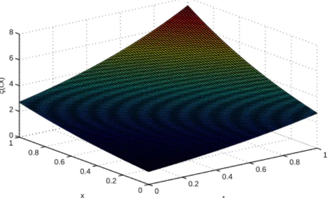
We see that our approximate solution is in coincide with the exact solution ξ(x, t) = Eα(xα)Eα(λtα). The Eq. (7.1)-(7.2) is calculated numerically for different values of α with λ= 1. The results of ξ(x, t) are presented in Figs. 1,2,3.
Example 7.2. Consider the following fractional diffusion-wave equation
∂αξ(x, t)
∂tα =λ
∂4αξ(x, t)
∂x4α , 0< α <2,
(7.6)
ξ(x,0) = cosα(xα), ∂
∂tξ(x,0) = 0,
0 0.2
0.4 0.6
0.8 1
0 0.2 0.4 0.6 0.8 1 0 2 4 6 8
t x
ξ
(t,x)
Figure 1. Plot of the approximation ξ(x, t) for α = 1
and λ= 1.
0 0.2
0.4 0.6
0.8 1
0 0.2 0.4 0.6 0.8 1 0 2 4 6 8 10
t x
ξ
(t,x)
Figure 2. Plot of the approximationξ(x, t) forα= 0.9
and λ= 1.
where the cos function in fractional sence is defined as
(7.8) cosα(xα) =
∞ ∑ k=0
(−1)kx2αk
0 0.2
0.4 0.6
0.8 1
0 0.2 0.4 0.6 0.8 1 0 2 4 6 8 10 12
t x
ξ
(t,x)
Figure 3. Plot of the approximationξ(x, t) for α= 0.8
and λ= 1.
As before, the second initial condition is forα >1 only. From (2.5)-(2.6) and by imposing the initial conditions, we have
(7.9) ξj+1(x, t) = cosα(xα) + λ
Γ(α)
∫ t 0
(t−τ)α−1∂
4αξ j(x, τ) ∂x4α dτ.
Hence
ξj(x, t) = cosα(xα) j ∑ k=0
λktkα γ(1 +kα), (7.10)
and therefore
(7.11) ξ(x, t) = lim
j→∞ξj(x, t) = cosα(x
α)Eα(λtα),
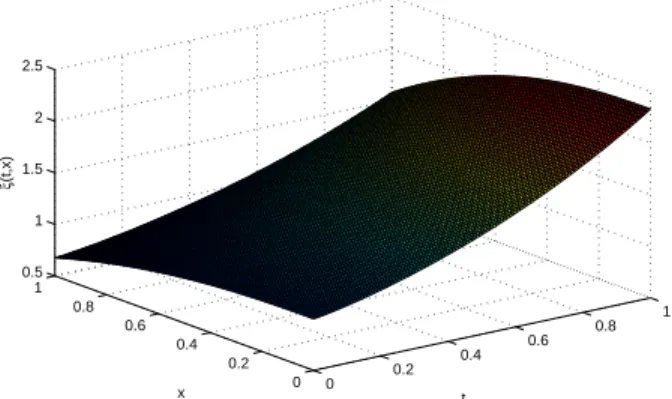
which is an exact solution of the given fractional diffusion wave Eq. (7.6)-(7.7). This equation is calculated numerically for different values ofα withλ= 1. The results ofξ(x, t) are presented in Figs. 4,5,6.
8. Conclusions
In this manuscript, the STIM has been successfully applied to com-pute the approximate analytical solution of the fractional diffusion-wave equations. The convergence and stability of the method, as applied to this equation have been thoroughly investigated. The obtained results show that, our approach provides the solution in terms of convergent series with easily computable components in a direct way and is very
0 0.2
0.4 0.6
0.8 1
0 0.2 0.4 0.6 0.8 1 0.5 1 1.5 2 2.5 3
t x
ξ
(t,x)
Figure 4. Plot of the approximation ξ(x, t) for α = 1
and λ= 1.
0 0.2
0.4 0.6
0.8 1
0 0.2 0.4 0.6 0.8 1 0.5 1 1.5 2 2.5 3
t x
ξ
(t,x)
Figure 5. Plot of the approximationξ(x, t) forα= 1.1
and λ= 1.
effective and convenient for dealing with the fractional diffusion-wave equations. Since we need to find just a few terms of the series, then the rest will be determined, automatically.
References
[1] O. P. Agrawal, A general solution for a fourth-order fractional diffusion-wave equation defined in a bounded domain, Computers and Structures 79 (2001), 1497–1501.
0 0.2
0.4 0.6
0.8 1
0 0.2 0.4 0.6 0.8 1 0.5 1 1.5 2 2.5
t x
ξ
(t,x)
Figure 6. Plot of the approximationξ(x, t) for α= 1.2
and λ= 1.
[2] F. B. M. Belgacemand, A. A. Karaballi, Sumudu transform fundamental properties investigations and applications, Journal of Applied Mathematics and Stochastic Analysis, 2006,Article ID 91083, (2006), 1-23.
[3] V. B. L. Chaurasia, J. Singh, Application of Sumudu transform in Schr¨odinger equation occurring in quantum mechanics, Applied Mathemati-cal Sciences 4 (2010), 2843-2850.
[4] A. Golbabai, K. Sayevand, Fractional calculus - A new approach to the analysis of generalized fourth-order diffusion-wave equations, Comput. Math. Appl., 61 (2011), 2227–2231.
[5] A. Golbabai, K. Sayevand,Analytical treatment of differential equations with fractional coordinate derivatives, Comput. Math. Appl., 62 (2011), 1003– 1012.
[6] E. Hesameddini, H. Latifizadeh, Reconstruction of variational iteration al-gorithms using the Laplace transform, Int. J. Nonlinear Sci. Numer. Simul. 10 (2009), 1377-1382.
[7] A. A. Kilbas, A. A. Koroleva, S.V. Rogosin, Multi-parametric Mittag-Leer functions and their extension, Fract. Calc. Appl. Anal., 16 (2) (2013), 378-404.
[8] V. Kiryakova,The multi-index Mittag-Leer functions as an important class of special functions of fractional calculus, Comput. Math. Appl., 59 (2010), 1885-1895.
[9] F. Mainardi,The fundamental solutions for the fractional diffusion-wave equa-tion, Appl. Math. Lett., 9 (1996), 23–28.
[10] I. Podlubny,Fractional differential equations, Academic Press, San Diego, 1999.
[11] K. Sayevand, A. Golbabai, Ahmet Yildirim,Analysis of differential equa-tions of fractional order, Appl. Math. Model., 36 (2012), 4356–4364.
[12] K. Sayevand, K. Pichaghchi, Successive approximation: A survey on stable manifold of fractional differential systems, Fract. Calc. Appl. Anal., 18 (3) (2015), 621–641.
[13] J. Tenreiro Machado, V. Kiryakova, F. Mainardi,Recent history of frac-tional calculus, Commun. Nonlinear Sci. Numer. Simu., 16 (2011), 1140– 1153.
Khosro Sayevand and Kazem Pichaghchi
Faculty of Mathematical Sciences, Malayer University, P. O. Box 16846-13114 Malayer, Iran