Sharif University of Technology
Scientia IranicaTransactions E: Industrial Engineering www.scientiairanica.com
Economic-statistical design of adaptive X-bar control
chart: a Taguchi loss function approach
F. Amiri
;1, K. Noghondarian and R. Noorossana
Department of Industrial Engineering, Iran University of Science and Technology, Tehran, 1684613114, Iran. Received 30 January 2013; received in revised form 19 March 2013; accepted 9 June 2013
KEYWORDS Adaptive control chart;
Variable sample size; Variable sampling interval;
Taguchi loss function; Economic-statistical design.
Abstract. Along with the widespread use of Taguchi methods in product design, denition of the loss function has been integrated with numerous models which require quality cost estimation. In this paper, the economic-statistical design of a variable sampling X-bar control chart is extended using the Taguchi loss function to improve chart eectiveness from a quality cost point of view. The eectiveness of the proposed schemes is evaluated by comparing optimal expected costs and statistical performance with each other and with the xed sampling policy. Results indicate a satisfactory performance for the proposed models.
c
2014 Sharif University of Technology. All rights reserved.
1. Introduction
Variability is an intrinsic characteristic of any produc-tion or service process. Generally speaking, process variation can be classied into two major categories of common cause and special cause. The common or chance cause variation is an inherent part of any process and can only be altered if the process nature itself is altered. On the other hand, special or assignable causes of variation are unusual disruptions in the process which should be removed immediately in order to bring the process under statistical control. The principal function of a control chart is to help the management distinguish between these two dierent sources of variation.
To design a control chart to monitor a process, sample size (n), sampling interval (h), and control limit coecient (k) should be determined. A control
1. Present address: Kermanshah University of Technology, Kermanshah, 6376667178, Iran.
*. Corresponding author. Tel.: +98 21 73225015; Fax: +98 21 73225098
E-mail addresses: f [email protected] (F. Amiri); [email protected] (K. Noghondarian); [email protected] (R. Noorossana).
char is referred to as Fixed Ratio Sampling (FRS), when samples of xed size at xed sampling intervals are obtained from the process. When any of these parameters are allowed to vary, then the control chart is referred to as an adaptive control chart. Adap-tive control charts lead to improved statistical results compared to sixed ratio sampling control charts [1,2]. Variable Sample Size (VSS), Variable Sampling In-terval (VSI), and Variable Sample Size and Sam-pling Interval (VSSI) are examples of adaptive control schemes.
Statistical and economical designs of control charts are two main approaches to design an optimum control chart. The statistical approach focuses on chart statistical performance. However, in the economic design of control charts, the emphasis is on economic issues, such as the cost associated with sampling and inspection, the cost associated with investigating an out-of-control signal and repairing the process, and the cost associated with producing nonconforming products. In order to design a control scheme with im-proved performance, with respect to both viewpoints, the economic-statistical design of control schemes was proposed by researchers.
of an X control chart with a VSI scheme. The economic design of a VSS Shewhart chart was developed by Park and Reynolds [4]. Economically designed VSSI Shewhart charts were considered by Das and Jain [5] and Park and Reynolds [4]. Yu and Chen [6] focused on designing a VSI X control chart in a continuous process. Lin et al. [7] and Chen and Yeh [8] extended the economic design of adaptive control charts for the case of non-normal observations. Several studies contributed to the development of the economic design of adaptive control charts [1,3,9-15].
Moreover, the Taguchi loss function, which con-siders loss to society as a quadratic function of product quality, has been used by many researchers to develop control schemes. This is in concordance with the main principle of six sigma methodology, where the main object is to reduce deviations around the tar-get. Several researchers have applied the loss function approach in the economic design of control charts. Alexander et al. [16] studied an economic model for an X control chart with the Taguchi loss function. Serel and Moskowitz [17] used the Taguchi loss function to develop the joint economic design of an Exponentially Weighted Moving Average (EWMA) for mean and variance. Niaki et al. [18,19] extended the Lorenzen-Vance [20] cost function using the multivariate Taguchi loss approach. Recently, Yeong et al. [21] studied eco-nomic and ecoeco-nomic statistical designs of the synthetic chart using loss functions.
This paper focuses on extending the X control chart with an adaptive scheme considering the Taguchi quality loss function. The remainder of this paper is organized as follows. In Section 2, the adaptive X control chart is developed. Section 3 describes the proposed algorithm. In Section 4, an illustrative example is given to evaluate the performance of the proposed methodology. Our conclusion is provided in the nal section.
2. Adaptive X control chart
In an adaptive X control chart, in addition to the usual control limit with coecient LX, a warning limit, denoted by wX, is considered. In the VSSI scheme, usu-ally, two sampling intervals, h2 < h1, and two sample
sizes, n1< n2 , are used. Sampling size and sampling
interval are established based on the position of the rst sampling statistic on the chart. In this regard, if the prior sample mean (i 1) falls in the warning region, the chart design (n2; h2; LX; wX) should be used for
the current sample point (i). Alternatively, if the prior sample point (i 1) falls in the central region, the chart design (n1; h1; LX; wX) should be employed for
the current sample point (i). When n1 = n2 = n and
h2< h1, then, VSSI X simplies to the VSI X chart.
When n1< n < n2and h1= h2= h, the VSSI X chart
reduces to the VSS X chart. Hence, the VSSI control scheme can be dened as follows:
(hi;ni; LX; wX) =
(
(h1; n1; LX; wX) if Xi 12 central region
(h2; n2; LX; wX) if Xi 12 warning region(1)
An important statistical measure, which deter-mines the performance of an adaptive control chart, is the adjusted average time to signal or AATS. If the assignable cause occurs according to an exponential distribution with parameter , then, the expected time interval in which the process remains in control is 1=. Hence, AATS can be dened as:
AAT S = AT C 1
; (2)
where the Average Time of Cycle (ATC) is the av-erage time from the start of production until the rst signal after the process shift. The memory less property of the exponential distribution allows the computation of the ATC using the Markov chain approach [22].
2.1. Markov chain approach
According to the VSSI scheme, at each sampling stage, one of the following transient states is met, according to the status of the process (in or out-of-control), size of the sample (small or large) and sampling frequency (short or long). The process is in state 1, if the prior sample point (i 1) falls in the central region or the process is actually in-control.
State 1: Position of sample statistic is jZj w and the process is in-control;
State 2: Position of sample statistic is w < jZj k and the process is in-control;
State 3: Position of sample statistic is jZj w and the process is out-of-control;
State 4: Position of sample statistic is w < jZj k and the process is out-of-control;
State 5: Position of sample statistic is jZj > k and the process is out-of-control (true alarm state).
If the position of the sample statistic is jZj > k while the process status is out-of-control, then a true alarm is signaled and the absorbing state (State 5) is arrived. In order to model the VSSI scheme based on the Markov chain approach, transition probabilities, pij
(i is the prior state and j is the current state), should be dened. The transition probability matrix, P = [pij],
p = 2 6 6 6 6 4
p11 p12 p13 p14 p15
p21 p22 p23 p24 p25
0 0 p33 p34 p35
0 0 p43 p44 p45
0 0 0 0 1 3 7 7 7 7
5; (3)
where the transition probabilities are dened as: p11= Pr(jZj wj jZj k) e h1;
p12= Pr(w < jZj kj jZj k) e h2;
p13= Pr(jZj wj jZj k) (1 e h1);
p14= 1 p11 p12 p13;
p21= Pr(jZj wj jZj k) e h1;
p22= Pr(w < jZj kj jZj k) e h2;
p23= Pr(jZj wj jZj k) (1 e h1);
p24= 1 p21 p22 p23;
p31= p32= 0;
p33= Pr(jY j wjY N(pn1; 1));
p34= Pr(w < jY j kjY N(pn1; 1));
p35= 1 p33 p34;
p41= p42= 0;
p43= Pr(jY j wjY N(pn1; 1));
p44= Pr(w < jY j kjY N(pn2; 1));
p45= 1 p43 p44: (4)
The product of the average number of visiting a transient state and the corresponding sampling interval determines the period, ATC.
ATC = b0(I Q) 1h; (5)
where I is the identity matrix of order four; b0 =
(p11; p12; p13; p14) is the vector of starting probability;
and Q is the transition matrix without elements asso-ciated with the absorbing state. h0 = (h
1; h2; h1; h2)
is the vector of sampling intervals corresponding to the transient states. The average number of samples (ANS) in the VSSI scheme is determined as follows:
ANS = b0(I Q) 1; (6)
where 0 = (n
1; n2; n1; n2) is the vector of the sample
sizes corresponding to the transition states. The
expected number of false alarms per cycle is given in Eq. (7):
ANS = b0(I Q) 1f; (7)
where f = (1; 2; 0; 0) is the vector of false alarms
probabilities in each transition state. 2.2. Taguchi loss function
In Taguchi philosophy, a loss incurs when the quality characteristic of interest deviates from its target value. The purpose of loss function is to reect the economic loss associated with variations and deviations from the target. Variation reduction is equivalent to lower loss and higher quality. Computation of production costs based on quadratic loss function, to economically design control charts, has been suggested by many au-thors [16,19,23-27]. In this paper, we also use Taguchi loss function, dened as L(X) = K(X T )2, where X is
a key quality characteristic, K is a positive coecient, and T is the target. Suppose the specication limits for the quality characteristic of interest are T and the cost of rework or scrap for one unit of product is A. The coecient, K, is dened as K = A
2.
When the process is in control, the quality charac-teristic, X, follows a normal distribution with mean 0
and variance 2
0. It is desirable for the location of the
in-control mean to coincide with the target location. However, if 0 is dierent from T , a xed bias impacts
all manufactured items. The expected quality cost per unit of product when the process is in control, J0,
is [27]:
J0= +1
Z
1
K(x T )2f(x)dx = +1
Z
1
K(x 0+ 0 T )2
f(x)dx = K[2
0+ (0 T )2]: (8)
When an assignable cause occurs, the process mean shifts to 1 = 0+ 0. The expected quality cost per
unit when the process is out of control, J1, is given by:
J1= +1
Z
1
K(x 1+ 1 T )2f(x)dx
=
+1
Z
1
K(x 0 0+ 0+ 0 T )2f(x)dx
= K[2
0+ (0 T )2+ 202 20(0 T )]: (9)
2.3. Cost model
Following renewal reward process assumption, the ex-pected quality cost per hour is computed as the ratio of the expected cost per cycle to the expected cycle
time. A quality cycle consists of one period when the process is in-control and two periods during an out-of-control state. The expected length of a quality cycle is calculated as follows:
ET = ATC + T0 ANF + T1: (10)
ET is composed of the in-control portion (including interruptions for false alarms) and the time to locate and repair the process, T1. T0 is the average time to
search when the process is in-control.
The costs of producing nonconformities while in- and out-of-control, sampling and inspection costs, costs of false alarms, and locating and removing an assignable cause are elements of the expected cost per cycle. Each individual cost element is derived as follows:
EC =C0(1=) + C1 (AATS) + s ANS
+ f0 ANF + W; (11)
where s is the sampling cost, f0 is the cost of false
alarms, and W is the cost associated with locating and repairing the process. Moreover, C0 and C1 are
the expected costs associated with producing non-conformities while the process is in-control and out-of-control, respectively. If p units are produced per hour, then, C0 = J0p and C1= J1p. The expected cost per
hour incurred by the process can be obtained as:
EA = EC
ET: (12)
In the economic-statistical design of an adaptive X control chart, the design vector consists of control limits, LX, warning lines, wX, sample sizes, n1and n2,
and sampling frequencies, h1 and h2. The objective is
to nd a design vector that minimizes EA, subject to some constraints. Hence, the optimization problem can be dened as:
Min EA(n1; n2; h1; h2; LX; wX)
Subject to : AATS AATSM;
ANF ANFM;
hmin h2< h1 hmax;
0 < w < L Lmax;
1 n1< n2 nmax (integers): (13)
In the optimization model, constraints ANF ANFM
and AATS AATSM are added to form the best
protection against false alarms and to detect process shifts as quickly as possible. The minimum and maximum values of possible sampling intervals between successive samples, hmin and hmax, are added to keep
the chart more practical. In this research, the values of hmin = 0:01 and hmax = 8 are used because sampling
intervals less than 0.01 and greater than 8 hours may be awkward in a work shift.
3. Solution algorithm
The economic-statistical optimization model has some discrete and continuous decision variables. Hence, the Genetic Algorithm (GA), which has been used in several studies, can be considered to optimize this problem [19,27-31]. The objective of GA is to obtain a global optimum solution. GA starts to generate a new generation or population using a collection of small possible solutions in a parallel process. The quality of solutions presented by GA depends on GA parameters. GA parameters are population size (Npop), crossover
(CP), Number of Elite (NE), Number of Generations (GN), and mutation rate. The key parameters, which should be determined at the beginning of the algorithm and should be used while applying the algorithm, are described below.
GA starts to work using some possible initial solutions referred to as \initial population". Each population has Npopchromosomes, which are produced
from the solution. In this research, each chromosome consists of ve genes, each of which is representative of a decision variable. The decision variable of the model includes (n1; n2; h1; h2; LX; wX).
The cost function is calculated for the chromo-somes of each generation. The best chromochromo-somes will be selected for crossover purposes. Each generation includes the Xkeep superior chromosome and Npop
Xkeep children, which have been generated through the
crossover.
The mutation operator is employed to prevent the GA from converging into a local optimum value. Selected chromosomes for mutation are not among the best of each generation essentially. The elite of each generation will be transferred directly to the next gen-eration to prevent losing the best chromosomes. The elitism operator is actually a method for maintaining the best chromosomes of each generation. After the mutation, for each chromosome, the cost function will be calculated. Then, the chromosomes will be ranked. The stopping criterion, the number of iterations in the algorithm, will be investigated, and the loop will continue until an optimum solution is obtained.
In the algorithm developed in this paper, mu-tation rate is considered a liner combination of the other parameters. The optimized combination of GA parameters is often accomplished using a trial and
error method, which is a hard process, due to the multiplicity of possible states. The optimum values for four GA parameters have been determined using Taguchi orthogonal array. Many analysts in the eld of Economic-Statistical Design (ESD) of control charts have already recommended using this method to determine the optimum value of GA parameters [22,29]. Nine combinations of control parameters in three dif-ference levels will be considered by L9 orthogonal array. Table 1 shows the value for each of the parameters.
The algorithm iterated three times (Y 1,Y 2, and Y 3) for each of the levels. Then the results are obtained from running the algorithm for 27 times. Since the objective function for the problem is a minimizing one, the signal-to-noise ratio (SN), dened as below, is calculated to evaluate the results of the experiments.
SN = 10 log
1 r
r
X
i=1
Y2 i
: (14)
In Eq. (14), r is the number of replicates for each level. Solution values for each level of parameters and the SN value for each level is tabulated in Table 2. The sum of the SN ratio for each level of the GA parameters is
shown in Table 3. The optimized combination of the levels of four GA parameters, Npop = 500, CF = 0:5,
NE = 6 and NG = 100, are recommended, based on the maximum of SN for each level.
4. Numerical analysis
To illustrate the application of the developed adaptive X control chart, numerical analysis has been under-taken. Logical ranges for each of the control chart parameters: Sampling size, sampling interval, and control limit coecient range, have been considered to be [1,30],[0.1,8] and [1,5], respectively. Cost and process parameters are as follows: Sampling cost is s = 5$, cost of detecting a reasonable deviation is W = 1000$, cost of false signal is f0 = 1500, average
time to search for a false signal is T0= 5 hour, and the
average time to detect the deviations and modify the process is T1 = 2 hour; process mean increases by 1.5
standard deviation ( = 1:5).
Also, the quadratic loss function coecient is K = 1, the actual process average is equal to the characteristic's target value, and the process variance is 2
0 = 1. The average process in-control period is
Table 1. Levels for each of the model parameters.
Parameter Range Level 1 Level 2 Level 3 Population size (Npop) 100-900 100 500 900 Crossover Fraction (CF) 0.1-0.9 0.1 0.50 0.90
Number of Elites (NE) 4-10 4 6 10
Number of Generations (NG) 50-150 50 100 150 Table 2. The objective values for each level of GA parameters.
Runs Npop CF NE NG Y 1 Y 2 Y 3 SN
1 100 0.10 2 50 121.848 123.106 123.106 -41.7760 2 100 0.50 6 100 121.848 123.106 121.848 -41.7463 3 100 0.90 10 150 123.106 123.106 123.106 -41.8056 4 500 0.10 6 150 121.848 121.848 121.848 -41.7164 5 500 0.50 10 50 121.848 121.848 121.848 -41.7164 6 500 0.90 2 100 121.848 121.848 121.848 -41.7164 7 900 0.10 10 100 121.848 121.848 121.848 -41.7164 8 900 0.50 2 150 121.848 121.848 121.848 -41.7164 9 900 0.90 6 50 121.848 121.848 121.848 -41.7164
Table 3. The sum of SN ratio for each level of GA parameters.
Npop CF NE NG
Level 1 -125.3279 -125.2088 -125.2088 -125.2088 Level 2 -125.1491* -125.1790* -125.1790* -125.1790* Level 3 -125.1491* -125.2383 -125.2383 -125.2383 * largest sum of SN ratio for each parameter within dierent levels [33].
equal to 100. If the production rate is equal to Pr = 100, the production cost for each defective product, while the process is under in-control and out-of-control conditions, will be equal to C0 = 100J0 and C1 =
100J1, respectively.
In the proposed model, solutions are evaluated based on the objective function of quality costs. The minimum cost solution for xed ratio sampling is (n; h; LX) = (4; 8:0; 2:15), with the cost equal to $119.50, where the average number of false signals is equal to ANFClassic = 0:375, and the adjusted
average time to signal is equal to AATSClassic = 60:0
hours. However, the VSSI scheme solution vector is (n1; n2; h1; h2; LX; wX). The optimum economic costs
achieved by solution vector (n1; n2; h1; h2; LX; wX) =
(1; 22; 8:00; 8:00; 2:43; 1:30), which will result in a cost equal to $118.60. In this scheme, ANFVSSI= 0:183 and
AATSVSSI = 46:55 hours are obtained. The optimum
VSI scheme is equal to (n1; n2; h1; h2; LX; wX) =
(4; 4; 8:00; 0:10; 2:19; 1:75). This scheme results in a cost equal to $119.45, ANFVSI=0:361, and AATSVSI=
56:69 hours. On the other hand, the optimum economic cost of the VSS scheme achieved by the solution vector (n1; n2; h1; h2; LX; wX) = (1; 23; 8:00; 8:00; 2:44; 1:23)
is $118.60 per hour, with ANFVSS = 0:177 and
AATSVSS= 46:63 hours.
Comparison of the adaptive schemes with the FRS scheme shows the eciency of the proposed model. Cost reduction due to using the VSSI plan is equal to 119:50 118:60
119:50 = 0:8%. Furthermore, the average
number of false signals has remarkably decreased to ANFVSSI = 0:183 from ANFClassic = 0:375 (51.20
% improvement). The AATSClassic = 60:0 hours has
reduced to AATSVSSI = 46:55 hours, which indicates
22.42% improvement. For this process shift size, the VSS scheme performs as well as the VSSI scheme, in terms of both cost and statistical measures. The VSI scheme shows better performance compared to the FRS scheme, but the dierence is not signicant. Since a control chart is designed to detect a variety of shift sizes in the process mean, other shift sizes need to be inves-tigated and this will be examined in the next section.
5. Sensitivity analysis
Investigation of the eects of changes in the esti-mated values of model parameters has been recom-mended in previous studies [19,32]. In this section, the eect of the process mean shift of sizes 2 f0; 5; 1; 0; 1; 5; 2; 0; 2; 5; 3; 0g will be evaluated.
The optimum solutions of adaptive schemes for dierent process mean shift sizes are tabulated in Tables 4 to 6. As shown in Table 4, the corresponding cost for small process mean shifts is less than the cost value for larger shift values. However, the proposed model oers better AATS for larger shift values, which will result in early identication of assignable causes.
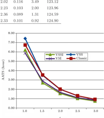
Also, the optimum solutions of the classic scheme are evaluated for dierent process mean shift sizes. The eect of process mean shift on the optimum solution of the classic scheme is summarized in Table 7. The performance of each adaptive scheme when the process is facing dierent shift sizes can be concluded by comparing these results. To better understand the dierence in each scheme, the cost and AATS of each scheme are compared in Figures 1 and 2, respectively.
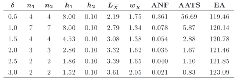
Table 4. Eect of process mean shift on the optimum solution of the VSI scheme.
n1 n2 h1 h2 LX wX ANF AATS EA
0.5 4 4 8.00 0.10 2.19 1.75 0.361 56.69 119.46 1.0 7 7 8.00 0.10 2.79 1.34 0.078 5.87 120.14 1.5 4 4 4.53 0.10 3.08 1.38 0.054 2.88 120.78 2.0 3 3 2.86 0.10 3.32 1.62 0.035 1.67 121.46 2.5 2 2 1.86 0.10 3.39 1.65 0.040 1.10 121.85 3.0 2 2 1.52 0.10 3.61 2.05 0.021 0.83 123.09 Table 5. Eect of process mean shift on the optimum solution of the VSS scheme.
n1 n2 h1 h2 LX wX ANF AATS EA
0.5 1 22 8.00 8.00 2.43 1.30 0.183 46.55 118.60 1.0 5 11 7.73 0.10 3.01 1.39 0.040 6.22 119.65 1.5 3 6 3.80 0.10 3.33 1.51 0.026 2.70 120.14 2.0 2 4 2.28 0.10 3.51 1.61 0.021 1.56 120.56 2.5 1 3 1.25 0.10 3.70 1.61 0.019 1.02 120.77 3.0 1 2 1.07 0.10 3.64 1.68 0.028 0.75 121.28
Table 6. Eect of process mean shift on the optimum solution of the VSSI scheme.
n1 n2 h1 h2 LX wX ANF AATS EA
0.5 1 23 8.00 8.00 2.44 1.32 0.177 46.63 118.60 1.0 8 14 8.00 8.00 2.51 1.57 0.145 7.43 121.77 1.5 6 9 5.06 5.06 2.75 2.02 0.116 3.49 123.12 2.0 4 6 3.05 3.05 2.95 2.23 0.103 2.00 123.96 2.5 3 4 2.13 2.13 3.10 2.36 0.089 1.31 124.59 3.0 2 3 1.41 1.41 3.19 2.33 0.101 0.92 124.90 Table 7. Eect of process mean shift on the optimum
solution of classic scheme.
n h LX ANF AATS EA
0.5 4 8.00 2.15 0.375 60.00 119.50 1.0 10 8.00 2.49 0.153 6.74 122.06 1.5 6 5.07 2.69 0.139 3.53 123.25 2.0 4 3.06 2.90 0.121 2.02 124.07 2.5 3 2.13 3.07 0.099 1.32 124.66 3.0 2 1.41 3.14 0.121 0.93 125.06
Figure 1. Comparison of cost in adaptive and classic schemes.
As shown in Figures 1 and 2, when a small shift (i.e. 0.5 standard deviation) incurs in the process, VSSI and VSS perform better compared to VSI and classic schemes. However, when the process is faced with moderate or large shift sizes (i.e. 1 or 2 standard deviation), VSSI and VSI schemes are always superior to VSS and classic schemes, in terms of both cost and AATS.
6. Conclusions
In this research, adaptive X control charts are devel-oped to monitor process mean, while process operating costs and deviation from the target are considered
Figure 2. Comparison of AATS in adaptive and classic schemes.
simultaneously. The relationship between process mon-itoring costs and deviations from the designed target value is incorporated in the model considering Taguchi loss function. Adaptive schemes, consisting of VSS, VSI, and VSSI schemes, are compared with the classic FRS scheme. Evaluation of the optimum solutions shows that shift size in the process mean inuences expected cost, as well as adjusted average time to signal. The proposed adaptive schemes remarkably improve both quality cost and alarm rates. Sensitivity analyses of the proposed model show that VSSI and VSS perform better in comparison to VSI and classic schemes when the chart is optimized for identifying small shifts in the process. However, VSSI and VSI schemes are always better than VSS and classic schemes when the process is facing moderate or large shift sizes. Hence, one can conclude that the proposed adaptive schemes are superior to the FRS scheme, in both aspects of process monitoring costs and statistical measures.
References
1. Nenes, G. \A new approach for the economic design of fully adaptive control charts", Int. J. of Production Economics, 131(2), pp. 631-642 (2011).
2. Faraz, A. and Saniga, E. \Economic statistical design of a T2 control chart with double warning lines", Int. J. of Quality and Reliability Engineering, 27(2), pp. 125-139 (2011).
3. Bai, D.S. and K.T. Lee \An economic design of variable sampling interval X control charts", Int. J. of Production Economics, 54(1), pp. 57-64 (1998).
4. Park, C. and Reynolds Jr. M.R. \Economic design of a variable sampling rate X chart", Int. J. of Quality Technology, 31(4), pp. 427-443 (1999).
5. Das, T.K. and Jain, V. \An economic design model for X charts with random sampling policies", IIE Transactions, 29(6), pp. 507-518 (1997).
6. Yu, F.J. and Chen, Y.S. \An economic design for a variable-sampling-interval X-bar control chart for a continuous-ow process", Int. J. of Advanced Manu-facturing Technology, 25(3-4), pp. 370-376 (2005).
7. Lin, H.H., Chou, C.Y. and Lai, W.T. \Economic design of variable sampling intervals X charts with A&L switching rule using genetic algorithms", Expert Systems with Applications, 36(2 PART 2), pp. 3048-3055 (2009).
8. Chen, F.L. and Yeh, C.H. \Economic statistical design for X-bar control charts under non-normal distributed data with Weibull in-control time", Int. J. of the Op-erational Research Society, 62(4), pp. 750-759 (2011).
9. Chen, Y.K. \Economic design of X control charts for non-normal data using variable sampling policy", Int. J. of Production Economics, 92(1), pp. 61-74 (2004).
10. Chen, Y.K., Hsieh, K.L. and Chang, C.C. \Economic design of the VSSI X-bar control charts for correlated data", Int. J. of Production Economics, 107(2), pp. 528-539 (2007).
11. Yu, F.J., Rahim, M.A. and Chin, H. \Economic design of VSI X control charts", Int. J. of Production Research, 45(23), pp. 5639-5648 (2007).
12. Li, F.C., Chao, T.C., Yeh, L.L. and Chen, Y. F. \The restrictions in economic design model for an x-bar control chart under non-normally distributed data with weibull shock model", in IEEM 2009 - IEEE International Conference on Industrial Engineering and Engineering Management, Hong Kong (2009).
13. Chen, F.L. and Yeh, C.H. \Economic design of VSI x-bar control charts for non normally distributed data under Gamma (; 2) failure models", Communications in Statistics - Theory and Methods, 39(10), pp. 1743-1760 (2010).
14. Niaki, S.T.A., Gazaneh, F.M. and Karimifar, J. \Eco-nomic design of x-bar control chart with variable sample size and sampling interval under non-normality assumption", A Genetic Algorithm, Economic Compu-tation and Economic Cybernetics Studies and Research (2012).
15. Prabhu, S.S., Montgomery, D.C. and Runger, G.C. \Economic-statistical design of an adaptive X-bar
chart", Int. J. of Production Economics, 49, pp. 1-15 (1997).
16. Alexander, S.M., Dillman, M.A., Usher, J.S. and Damodaran, B. \Economic design of control charts us-ing the Taguchi loss function", Computers & Industrial Engineering, 28(3), pp. 671-679 (1995).
17. Serel, D.A. and Moskowitz, H. \Joint economic design of EWMA control charts for mean and variance", European Journal of Operational Research, 184(1), pp. 157-168 (2008).
18. Niaki, S.T.A., Malaki, M. and Ershadi, M.J. \A particle swarm optimization approach on economic and economic-statistical designs of MEWMA control charts", Scientia Iranica, 18(6), pp. 1529-1536 (2011).
19. Niaki, S., Ershadi, M. and Malaki, M. \Economic and economic-statistical designs of MEWMA control charts - A hybrid Taguchi loss, Markov chain, and genetic al-gorithm approach", Int. J. of Advanced Manufacturing Technology, 48(1), pp. 283-296 (2010).
20. Lorenzen, T.J. and Vance, L.C. \The economic design of control charts: A unied approach", Technometrics, 28(1), pp. 3-10 (1986).
21. Yeong, W.C., Khoo, M.B.C., Lee, M.H. and Rahim, M.A. \Economic and economic statistical designs of the synthetic X-bar chart using loss functions", Euro-pean Journal of Operational Research, 48, pp. 571-581 (2013).
22. Chen, Y.K. and Chang, H.H. \Economic design of variable parameters X control charts for processes with fuzzy mean shifts", The Journal of the Operational Research Society, 59(8), pp. 1128-1135 (2008).
23. Moskowitz, H., Plante, R. and Chun, Y.H. \Eect of quality loss functions on the economic design of x pro-cess control charts", European Journal of Operational Research, 72(2), pp. 333-349 (1994).
24. Ben-Daya, M. and Duuaa, S.O. \Integration of Taguchi's loss function approach in the economic design of x
/
chart", Int. J. of Quality & Reliability Management, 20(5), pp. 607-619 (2003).25. Wu, Z., Shamsuzzaman, M. and Pan, E.S. \Opti-mization design of control charts based on Taguchi's loss function and random process shifts", Int. J. of Production Research, 42(2), pp. 379-390 (2004).
26. Serel, D.A. \Economic design of EWMA control charts based on loss function", Mathematical and Computer Modelling, 49(3-4), pp. 745-759 (2009).
27. Safaei, A., Kazemzadeh, R. and Niaki, S. \Multi-objective economic statistical design of X-bar control chart considering Taguchi loss function", Int. J. of Advanced Manufacturing Technology, 59(9), pp. 1091-1101 (2012).
28. Lin, S.N., Chou, C.Y., Wang, S.L. and Liu, H.R. \Eco-nomic design of autoregressive moving average control chart using genetic algorithms", Expert Systems with Applications, 39, pp. 1793-1798 (2012).
29. Chou, C.Y., Cheng, J.C. and Lai, W.T. \Economic design of variable sampling intervals EWMA charts with sampling at xed times using genetic algorithms", Expert Systems with Applications, 34(1), pp. 419-426 (2008).
30. Shiau, Y.R. \Monitoring capability study and genetic economic design of X-bar control chart", Int. J. of Advanced Manufacturing Technology, 30(3-4), pp. 273-278 (2006).
31. Bakir, M.A. and Altunkaynak, B. \The optimization with the genetic algorithm approach of the multi-objective, joint economical design of the x and R control charts", Journal of Applied Statistics, 31(7), pp. 753-772 (2004).
32. Mortarino, C. \Duncan's model for Xbar-control charts: sensitivity analysis to input parameters". Int. J. of Quality and Reliability Engineering, 26(1), pp. 7-26 (2010).
33. Taguchi, G., Chowdhury, S. and Wu, Y., Taguchi's Quality Engineering Handbook, Hoboken, New Jersey, John Wiley & Sons, Inc (2005).
Biographies
Farzad Amiri received a BS degree in Civil Engineer-ing from Bu-Ali-Sina University, Hamedan, Iran, in 1994, an MS degree in Industrial Engineering (System Management and Productivity), in 2004, from the University of Science and Technology, Tehran, Iran, where he is currently pursuing a PhD degree. He is also Assistant Professor of Industrial Engineering at the University of Kermanshah, Iran. His research interests
include quality, statistical quality control, simulation and project management. He is member of the Iranian Industrial Engineering Society, Project Management Society and Civil Engineering Society.
Kazem Noghondarian received a BS degree in Busi-ness Administration from the University of Nevada, USA, an MS degree in Industrial Engineering from Arizona State University, USA, and a PhD degree in Mechanical Engineering from the University of British Colombia, USA. He is currently Assistant Professor of Industrial Engineering at Iran University of Science and Technology (IUST), Tehran, Iran. He has pub-lished over 30 research papers. His research interests in-clude statistical quality control, design of experiments, econometrics and intelligent quality engineering. Rassoul Noorossana received his BS degree in En-gineering from Louisiana State University, USA, in 1983, and MS and PhD degrees in Engineering Man-agement and Applied Statistics from the University of Louisiana, in 1986 and 1990, respectively. He is cur-rently Professor of Applied Statistics at Iran University of Science and Technology, Tehran, Iran. His primary research interests include statistical process control, process optimization, statistical prole monitoring, and statistical analysis. He is Editor of the Journal of Industrial Engineering International and serves on the editorial review board of many other journals. He is also senior member of the American Society for Quality, Iranian Society for Quality, Iranian Statistical Association, and the Industrial Engineering Society.