An Accurate Guidance Algorithm for Implementation Onboard Satellite Launch Vehicles

Vol. 17, No. 2, pp. 175{188 c

Sharif University of Technology, December 2010

An Accurate Guidance Algorithm

for Implementation Onboard

Satellite Launch Vehicles

M. Marrdonny

_{and M. Mobed}

Abstract. An algorithm for guiding a launch vehicle carrying a small satellite to a sun synchronous LEO is presented. Before the launch, a nominal path and the corresponding nominal control law for the entire journey are computed. For each sampling instant during the guided ight, a linear equation approximately relating the dierences between the actual and nominal values is considered, and a Least-Squares formula using data from on-line state measurements is applied to compute the actual control. The coecient matrices of the Least-Squares formula can be determined by o-line computations. The method enjoys simplicity of implementation by onboard computers, as well as robust accuracy against strong winds and uncertainties in thrust magnitude.

Keywords: Disturbance rejection; Guidance systems; Satellites; Optimal trajectory; Launch vehicle.

INTRODUCTION

Articial satellites are placed into Earth orbits using missiles known as \carrier rockets or launch vehicles". Some of the issues concerning commercial launch ve-hicles have been addressed in [1,2]. Today, launching satellites has become a vast and multifaceted endeavor with research continuing on its various aspects includ-ing rocket guidance.

In a previous work of the authors, a guidance algorithm was proposed in which the so-called path-to-go and the corresponding control were recomputed at the juncture at which the rocket left the atmosphere and entered the exoatmosphere where atmospheric disturbances were supposed to be negligible or nonex-istent [3]. The main attribute of the recomputed path and control was that they were used as the nominal trajectory to be followed throughout the rest of the ight, and no further corrections were introduced once the new path-to-go and control became available. The algorithm was shown through simulations to work very well in the absence of exoatmospheric disturbances. However, since disturbances of various kinds do exist during all phases of the ight, it stands to reason

1. School of Electrical Engineering, Sharif University of Tech-nology, Tehran, P.O. Box 11155-9363, Iran.

*. Corresponding author. E-mail: [email protected]

Received 4 October 2009; received in revised form 18 April 2010; accepted 17 July 2010

to expect that even during the exoatmospheric ight, corrections to thee control could be used to improve precision. The present paper aims at continually providing such corrections in a manner as eciently as possible from the standpoint of the computational burden imposed upon the onboard computer. The term \computational burden" has been used rather loosely here to refer to any one or more of the concepts of computational eort, computational com-plexity, computational load etc. Given the nature of the problem under discussion, the number of sam-pling periods needed to obtain one sample of the control signal has been used as a measure of the computational burden. In the algorithm presented in this article, the control signal to be applied dur-ing the kth sampldur-ing period is computed durdur-ing the (k 1)th, according to a myopic policy, and this continues throughout the exoatmospheric phase until the moment of orbit insertion. As such, it takes only one sampling period to obtain each sample of the control signal. This is to be compared with [3] where several sampling periods were needed to com-plete the updating computations, which were done only once at the beginning of the exoatmospheric phase.

Guiding a satellite launch vehicle traditionally involves an open-loop phase for the endoatmospheric part, and a closed-loop phase for the exoatmospheric part of the ight. Moreover, it is sometimes helpful

to distinguish between the trajectory selection and the control issues of guidance. The trajectory, the control, or both, may be optimal or near-optimal, with respect to appropriate criteria. In this regard, the Linear Tangent Law (LTL) has been shown to have certain desirable properties [4,5].

Guidance computations fall into two categories: O-line and on-line. \O-line" refers to computations performed before the take-o of the launch vehicle. Usually, in o-line computations, an optimal or near-optimal trajectory and control law are found for the entire rocket mission before it leaves the launch pad. The trajectory thus determined is treated as the nominal or reference trajectory, and the corresponding control law may be applied to track and keep the vehicle near the reference trajectory during the guided ight. In nding the nominal trajectory and control, o-line computations must also take into account the structural limitations of the rocket's fuselage, which is longitudinally strong and laterally weak. This can be accomplished either by introducing constraints into the underlying thrust-controlled optimization, as in for example [6-9], or by using pitch-over and gravity-turn maneuvers, as in [10]. References [6,11-15] discuss some of the methods of computing the optimal trajectory. Methods of tracking the reference trajectory can be found in [7,8,11,14]. Some of the methods of imple-menting entirely closed-loop guidance laws have been discussed in [9,15-17]. These methods involve on-line computations.

The term \on-line" refers to computations per-formed by an onboard computer after the take-o. On-line guidance algorithms tend to be computationally demanding and challenging to implement on small- to medium-powered computers.

An important consideration, especially in the case of on-line guidance, is the availability of computation results in a short, denite time. However, convergence does not always hold in computations involving innite sequences of iterations. Even in cases where conver-gence does hold, its rate may be dicult to determine or estimate. Thus, algorithms that employ innite sequences of iterations for on-line computations seem to be of limited interest.

It is now possible to summarize the overall scheme as follows: O-line computations determine a nom-inal trajectory-and-control pair for the entire launch mission by using gravity-turn and LTL, respectively, for the endoatmospheric and exoatmospheric phases. During the vertical launch and the pitch-over maneu-ver, control is open-loop and it is as found previously by the o-line computations. The nominal trajectory remains in force for the entire ight period. However, control becomes closed-loop during the gravity-turn maneuver, and it stays closed-loop throughout the rest of the ight. The closed-loop control at each sampling

instant is realized via a gain matrix calculated by Least-Squares methods devised to minimize error at the next sampling instant.

The paper has been organized in seven sections. First three dimensional model of the launch vehicle is described. Then, the nominal ight path and the pro-posed guidance algorithm for closed-loop operation are introduced and its convergence is studied. Following that, simulation results of the proposed algorithm for a two-stage launch vehicle are discussed and, nally, concluding remarks are given.

PHYSICAL MODEL

Models of the launch vehicle, gravitational eld and atmosphere are exactly the same as those used in [3] from which this section has been taken almost verbatim and presented here for ease of reference.

A two-stage launch vehicle is considered. Each stage is powered by a liquid-propellant engine. The engines cannot be throttled. However, Thrust Vector Control (TVC) is possible. By design, the rst stage separates when its fuel is depleted and the second stage ignites. The objective is to insert a research satellite with a mass of 10-kg into a sun synchronous low Earth orbit at a height of 200 km. The three-degree-of-freedom equations of motion relative to the Earth are [18]:

_ = V cos cos _{r cos} ; (1)

_ = V cos sin _r ; (2)

_h = V sin ; (3)

_V = 1_m(T cos D mg sin

+ wEcos cos + wNcos sin + wUsin )

+ r!2_{cos (cos sin sin cos sin ); (4)}

_ = _mV1 [(T sin + L) cos mg cos wNsin sin wEsin cos + wUcos ]

+V cos _r + 2! cos cos

_ = _{mV cos} 1 [(T sin + L) sin + wEsin

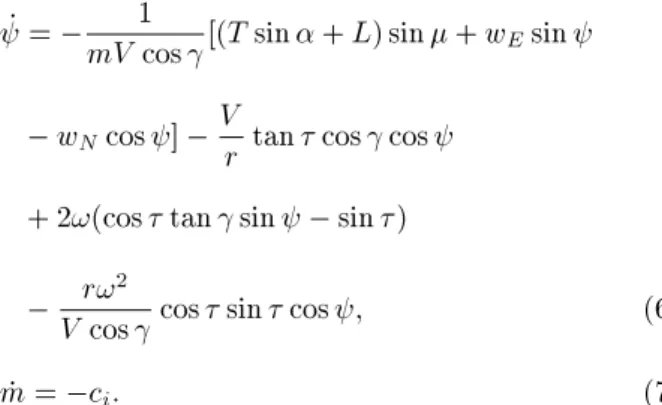
wNcos ] V_r tan cos cos

+ 2!(cos tan sin sin ) r!2

V cos cos sin cos ; (6)

_m = ci: (7)

In Equations 1-7, is the longitude, is the latitude, h is the altitude above mean sea level, V is the velocity, is the ight path angle, is the heading angle, m is the sum of the masses of the launch vehicle and the payload, r is the distance between the launch vehicle and the Earth centre, g is the local gravitational acceleration, ! is the rotational velocity of Earth, is the angle of attack, is the velocity roll angle, and T , D, L are the thrust, drag and lift magnitudes, respectively. Furthermore, wE, wN and wU are wind

force components in the east, north and up directions. Thus, wind force components have been introduced explicitly in the equations and not implicitly through aerodynamic forces. This allows for a more direct evaluation of the algorithm's performance against wind disturbances. Figure 1 depicts the coordinate frame in which the equations have been written.

The thrust model is given by:

T = Tvac pAe; (8)

where Tvac is the engine thrust in vacuum, p is

atmospheric pressure, and Ae is the exit area of the

engine.

The air density and pressure are modeled as the following exponential functions of altitude [18]:

= sexp

h h1

; (9)

p = psexp

h h2

; (10)

Figure 1. Coordinate frame.

where sand psare the air density and pressure at sea

level, and p are those at altitude h, and h1 and h2

are positive constants. The Earth is assumed to be a rotating, spherical body with an inverse squared law of gravity eld. The speed of sound is given using the perfect gas law:

a = r

p; (11)

where a is the speed of sound and is the ratio of specic heat of air. The dynamic pressure, q, the drag, D, and the lift, L, are given by:

q = 1

2V2; (12)

D = qAbCD; (13a)

L = qAbCL: (13b)

In the above, CD is the drag coecient, CL is the lift

coecient, and Abis the aerodynamic reference area of

the launch vehicle. The drag and lift coecients, CD

and CL, are modeled as polynomials in during the

rst stage:

CD= CD0(M) + CD1(M) + CD2(M)2

+ CD3(M)3; (14)

CL= CL1(M): (15)

Wind force components are given by:

wE=1₂E2ALCD; (16a)

wN = 1₂N2ALCD; (16b)

wU =1₂U2ALCD; (16c)

where E, N and U are the east, north and up

components of the wind speed, and AL is the lateral

cross section area of the launcher.

After staging, the vehicle will y at hypersonic velocities and aerodynamic force coecients will be independent of the Mach number. The aerodynamic models for the second stage are:

CD= CD0+ CD22; (17)

CL= CL1 + CL2jj: (18)

The drag and lift coecients in Equations 14, 15, 17 and 18 are obtained by applying interpolation techniques to tabular data [19]. In the dense part of the

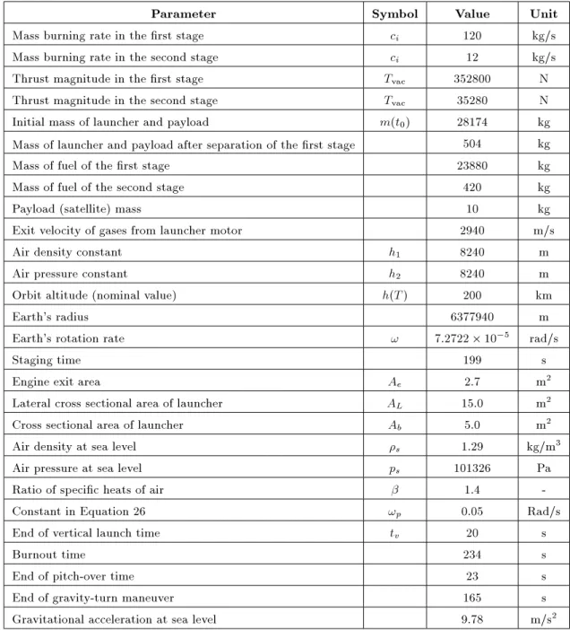
Table 1. Numerical value of the launch parameters.

Parameter Symbol Value Unit Mass burning rate in the rst stage ci 120 kg/s

Mass burning rate in the second stage ci 12 kg/s

Thrust magnitude in the rst stage Tvac 352800 N

Thrust magnitude in the second stage Tvac 35280 N

Initial mass of launcher and payload m(t0) 28174 kg

Mass of launcher and payload after separation of the rst stage 504 kg Mass of fuel of the rst stage 23880 kg Mass of fuel of the second stage 420 kg Payload (satellite) mass 10 kg Exit velocity of gases from launcher motor 2940 m/s Air density constant h1 8240 m

Air pressure constant h2 8240 m

Orbit altitude (nominal value) h(T ) 200 km

Earth's radius 6377940 m

Earth's rotation rate ! 7:2722 10 5 _rad/s

Staging time 199 s

Engine exit area Ae 2.7 m2

Lateral cross sectional area of launcher AL 15.0 m2

Cross sectional area of launcher Ab 5.0 m2

Air density at sea level s 1.29 kg/m3

Air pressure at sea level ps 101326 Pa

Ratio of specic heats of air 1.4 -Constant in Equation 26 !p 0.05 Rad/s

End of vertical launch time tv 20 s

Burnout time 234 s

End of pitch-over time 23 s

End of gravity-turn maneuver 165 s Gravitational acceleration at sea level 9.78 m/s2

atmosphere, the thrust and velocity vectors are almost aligned; therefore, the pitching moments are assumed negligible for both stages. Numerical values for the launch vehicle parameters are listed in Table 1.

The control variables are the angle of attack and the velocity roll angle . Therefore, the guidance system must have two outputs. As a matter of fact, in a model slightly more elaborate than Equations 1 to 7, and would themselves appear as state variables rather than controls. But, even then, and would have relatively fast dynamics and, thus, a good approximation may be obtained by considering them as control variables.

The singularities in Equations 5 and 6, due to

V = 0 at the take-o instant and = 90 deg during the vertical launch, are removed by modifying the equations of motion for the vertical launch segment, as follows:

_ = 0; (19)

_ = 0; (20)

_h = V; (21)

_V = 1_m(T D mg) + r!2_{; (22)}

_ = 0; (24)

_m = ci: (25)

NOMINAL PATH

The target orbit is a near-circular sun synchronous LEO at an altitude of 200 km above mean sea-level. The launch site is at latitude of 35 deg. The launch program consists of four segments in chronological order, as follows:

Segment 1 is the vertical ight. During this segment, control variables are kept at zero and the vehicle gains both altitude and speed. Take o occurs at a time instant when the launch site reaches the target orbit plane. This yields a planar nominal trajectory. Numerical values for the duration of Segment 1 and the altitude and speed at its end are, respectively, 20 s, 430 m and 44 m/s.

Segment 2 is the pitch-over maneuver during which the angle of attack is increased slightly from zero according to the following equation:

nom(t) = ₂ nom(t) !p(t t): (26)

The ight path angle decreases slightly and by the end of this segment it will be less than, but very close to, 90 deg. to prepare the vehicle for its next maneuver. The pitch-over maneuver lasts for 3 seconds. Numerical values for the time-independent constants, !p and t, are determined by

trial-and-error through simulation.

Segment 3 is the gravity-turn maneuver during which the control variables, and , are kept at zero to eliminate lateral aerodynamic forces and moments. Flight path angle, , decreases, and the vehicle completes its journey across the dense part of the atmosphere [10]. By the end of Segment 3, the vehicle will have gained altitude, velocity and a ight path angle sucient for the insertion maneuver to begin.

Segment 4 begins as soon as the vehicle leaves the atmosphere. Here, the aerodynamic forces and moments are negligible, and control through and becomes possible. O-line computations corresponding to this segment use, through the following equation, the Linear Tangent Law (LTL) of guidance for its simplicity, eectiveness and near optimality:

tan[nom(t) + nom(t)] = at + b: (27)

Parameters a and b are determined by satisfying two nal conditions of the powered ight, namely, nal

height and nal ight path angle: hnom(T ) = 200; 000 m;

nom(T ) = 0 deg. (28)

Final time T is the fuel depletion time of the second stage engine. The nominal value of (t) is identically zero throughout the powered ight, nom(t) 0,

because the launch site and hence the entire nom-inal trajectory are both on the target orbit plane. Using Newton's method, the numerical values of a and b of Equation 27 have been found to be a = 0:022739 s 1 _{and b = 4:657243. This concludes}

the last segment of o-line computations for nominal guidance.

CLOSED-LOOP GUIDANCE ALGORITHM The nominal path and its computation described in the previous section refer to ideal conditions where no disturbances are present. In reality, disturbances can distract the vehicle and even divert it from the nominal plane, resulting in nonplanar motion. Thus, in order to insert the satellite into its prescribed orbit as precisely as possible, both variables and should be used for control purposes, particularly during the exoatmospheric phase. A control law meeting this requirement will be devised directly in discrete time. However, it would be helpful to rst write the original continuous-time state-space equations more compactly in a vector form as follows:

_x(t) = [x(t); u(t); n(t)];

_xnom(t) = [xnom(t); unom(t); nnom(t)];

y(t) = `[x(t)];

ynom(t) = `[xnom(t)]; (29)

where nnom(t) 0 and the subscript \nom"

every-where refers to the nominal path. The state vector is x = [ h V m]0_{, the control vector is u = [ ]}0_,

the disturbance vector is n = [wE wN wD]0; : R12!

R7 _{and ` : R}7 _{! R}3 _{are xed known nonlinear}

functions, and y , [h (cos )(cos )]0 _{is the output}

vector in which (cos )(cos ) = cos i and i is the orbit inclination. Function is a composition of functions given by Equations 1-7 and several others, such as r, T , CL, CD, p, , q etc. Disturbance-induced perturbations

in state, output and control are given by: x(t) , x(t) xnom(t);

y(t) , y(t) ynom(t);

Because of structural constraints, the angle of at-tack during Segment 3 is kept near zero, hence, the guidance algorithm is almost open-loop during this segment, which is a substantial part of the path. The impact of disturbances is compensated mainly in Segment 4.

The analysis and design pertaining to Segment 4 are in discrete time. For the continuous-time processes of state x(t), output y(t), control u(t) and disturbance n(t), the notations x[k]; y[k]; u[k] and n[k] will be used to represent x(tk); y(tk); u(tk) and n(tk) where tk =

kt; t is the xed known sampling period, and k is an integer. At each sampling time during Segment 4, input vector u is determined so as to minimize a metric between y[k+1] and ynom[k+1]. To that end, y[k+1] is

rst written as function F of state vector x[k], control vector u[k] and disturbance vector n[k]:

y[k + 1] = F(x[k]; u[k]; n[k]): (31)

On linearizing F in Equation 31, by using Jacobians evaluated at the nominal path and using discrete-time versions of Equation 30, one arrives at the follow-ing expression for y[k + 1] as a linear function of x[k]; u[k] and n[k]:

y[k + 1] =@F_@x(Z(k))x[k] +@F_@u(Z(k))u[k]

+@F_@n(Z(k))n[k]; (32)

where Z(k) , (xnom[k]; unom[k]; 0) denotes the

nomi-nal path and controls.

On replacing the zero-mean random quantity n[k] in Equation 32 by its mean, that equation is further simplied as follows:

y[k + 1] =@F_@x(Z(k))x[k] +@F_@u(Z(k))u[k]: (33) Designing the control law is accomplished through minimization of errors. To compute u[k], the control to be applied at time t, one seeks to minimize, by an appropriate choice of u[k], the quantity

jjy[k + 1]jj2_{= jj}@F

@xx[k] + @F

@uu[k]jj2;

a measure of error at time t. However, the matrix

@F

@u(Z(k)) may in some cases be ill-conditioned or

singular. There is also the question of dierences among the output variables in their orders of mag-nitude, importance and dimension. Thus, instead of minimizing jjy[k + 1]jj2_{, one minimizes jjQy[k +}

1]jj2_{+ jjr}

uu[k]jj2 by choosing u[k] where ru is a

Tikhonov regularization parameter and Q a scaling

matrix. Treating this as a Least-Squares problem, the solution is given in terms of x[k] as:

u[k] = (A0_{[k]A[k] + r}2

uI) 1A0[k]B[k]x[k]; (34)

where:

A[k] = Q@F_@u(Z(k)); (35a)

B[k] = Q@F_@x(Z(k)): (35b)

The Jacobians in Equations 35 are computed o-line and numerically for every sampling time. Vector x[k] is computed through x[k] = x[k] xnom[k]

where, of course, nominal state xnom[k] is available

from o-line computations and the actual state, x[k], is measured during the ight using various sensors and measurement devices. The x[k] thus found is substituted in Equation 34 and u[k] is, thereby, computed. The control to be applied at time k is obtained from u[k] = u[k]+unom[k] where, again, the

nominal control is known from o-line computations. In consideration of structural limitations, the control variables are restricted to 1 deg while the launch vehicle is inside the atmosphere. The scaling matrix was taken to be Q = diag [10 5 _{1 1] in simulations.}

AN ANALYSIS OF ERROR

The results presented in the next section show how the closed-loop guidance algorithm succeeds in reducing, practically to zero, by the time of orbit insertion, the error between actual and nominal quantities of interest, which consist of altitude, h, ight path angle, , and orbit inclination, i. This is essentially the question of convergence to zero of the dierence between actual and nominal outputs: limt!1y(t) = 0, where

y(t) = y(t) ynom(t). Clearly, one would like such

convergence to hold not just for a few simulation runs corresponding to a few choices of initial state errors, but for all possible initial state errors, x(0), where x(0) = x(0) xnom(0). Thus, one would ideally like

to satisfy the following property or condition: lim

t!1y(t) = 0 8x(0) 2 B; (36)

where B is an open ball of nonzero radius centered at the origin of R7_{. The time t = 0 in x(0)}

in Equation 36, refers to the time of leaving the atmosphere after which there will be no forces of atmospheric disturbance. An analogy exists between Condition 36 and the denition of global asymptotic stability for a nominal solution of a dynamical system. However, there exists also an important distinction between the two. Condition 36 is concerned with

the convergence of y(t), whereas the said notion of stability traditionally addresses the convergence of x(t) = x(t) xnom(t). Whether Condition 36 is

regarded as a condition of convergence or of stability, and proposing such distinctions do not seem to be particularly fruitful anyway, it is hard to achieve an analytical proof of Condition 36, even with strong ad hoc assumptions. Therefore, we shall settle for the modest goal of computationally verifying a more tractable, yet important aspect of Condition 36, as explained in the sequel.

To begin, a discrete-time version of Equations 29 is obtained for the actual trajectory by applying Euler's forward approximation, _x x(t+T ) x(t)_t , at each epoch of discrete time, t = tk= kt:

x[k + 1] x[k]

t = (x[t]; u[t]; n[t]);

y[k] = `(x[k]): (37)

The approximation sign in Equations 37 may be re-placed by an equality sign in order to get the following set of state and output equations in discrete time:

x[k + 1] = (x[k]; u[k]; n[k]);

y[k + 1] = F(x[k]; u[k]; n[k]); (38)

where:

(x; u; n)def= t:(x; u; n);

F(x; u; n)def= `((x; u; n)); (39)

or F = ` . Function F in Equations 38 and 39 is the same as the one already encountered in Equation 31. Needless to say, x[k] and y[k] in Equations 38 and 39 and all subsequent equations only approximately represent x(kt) and y(kt), respectively. Such approximation is a result of having substituted in Equation 37 the sign by = and used, subsequently, in Equation 38, x[k], which is an approximation to x(kt) instead of x(kt) itself. For the discretization approximation to be good, t must be suciently small. A suitable value for t is determined through trial-and-error in simulations. Discrete-time equations of the nominal path are obtained in a like manner from Equations 29 and they correspond to n(t) = n[k] = 0. They are:

xnom[k + 1] = (xnom[k]; unom[k]; 0);

ynom[k + 1] = F(xnom[k]; unom[k]; 0): (40)

The idea is to consider, as state and output errors, the quantities x[k] = x[k] xnom[k] and y[k] =

y[k] ynom[k] instead of, respectively, x(t) and y(t),

alluded to before:

x[k + 1] = x[k + 1] xnom[k + 1]

= (x[k]; u[k]; n[k]) (xnom[k]; unom[k]; 0);

y[k + 1] = y[k + 1] ynom[k + 1]

= F(x[k]; u[k]; n[k])

F(xnom[k]; unom[k]; 0) : (41)

Under smoothness conditions on and F, Equatios 41 may be linearized with respect to the nominal path to yield:

x[t + 1] x(Z[k])x[k] + u(Z[k])u[k]

+ n(Z[k])n[k];

y[t + 1] Fx(Z[k])x[k] + Fu(Z[k])u[k]

+ Fn(Z[k])n[k]; (42)

where, of course, Z[k] , (xnom[k]; unom[k]; 0).

Nota-tion , instead of , will be used henceforth on account of the additional approximation introduced through linearization. This is done in order to emphasize the distinction between x[k] and x[k], between y[k] and y[k], and also between u[k] and u[k] where the sequences x[k], y[k] and u[k] are dened as being governed by the following sets of equations:

x[t + 1] x(Z[k])x[k] + u(Z[k])u[k]

+ n(Z[k])n[k];

y[t + 1] Fx(Z[k])x[k] + Fu(Z[k])u[k]

+ Fn(Z[k])n[k]: (43)

According to the result obtained previously in Equa-tion 34, quantity u[k] or more precisely u[k], is given by:

u[k] = G[k]x[k]; where:

G[k]def= (A0_{[k]A[k] + r}2

uI) 1A0[k]B[k]; (44)

where A[k] and B[k] are as in Equations 35. On substituting u[k] from Equation 44 into Relation 43, one will arrive at:

x[k + 1] = C[k]x[k] + D[k]n[k];

The coecient matrices in Equations 45 are given by the following denitions:

C[k]def= x(Z[k]) u(Z[k])G[k];

D[k]def= n(Z[k]);

K[k]def= Fx(Z[k]) Fu(Z[k])G[k];

L[k]def= Fn(Z[k]): (46)

By choosing k = 0 as the moment of departure from the atmosphere, one will get n[k] = 0 8k 0. Thus, Equations 45 simplies to x[k + 1] = C[k]x[k] and y[k+1] = K[k]x[k] from which it now readily follows that:

y[k + 1] = K[k]C[k 1] C[0]x[0] = M[k]x[0];

where:

M[k]def= K[k]C[k 1] C[0] 8k 1: (47) On taking the norms of both sides of y[k + 1] = M[k]x[0] and using a basic property of norms, there follows the inequality:

jjy[k + 1]jj jjM[k]jj jjx[0]jj: (48)

As shown in Figure 2, the graph of jjM[k]jj becomes rapidly decreasing with increasing k, as soon as the vehicle leaves the atmosphere. The graph also suggests jjM[k]jj converges to zero, as k ! 1. Since matrices C[k], K[k] and M[k] are predetermined and not depen-dent upon or aected by the actual trajectory or errors therein, it may be concluded that:

lim

k!1y[k] = 0 8x(0) 2 R

7_{: (49)}

Figure 2. jjM[k]jj monotonically decreases as k increases and it converges to zero as k ! 1.

The limiting property (Equation 49) asserts that in a linearized discrete-time model, the closed-loop control law obtained from u[k] = G[k]x[k] does indeed bring the actual output variables very close to the desired, i.e. nominal values for all errors in the initial state vector. Therefore, it is possible to conclude that, if the sampling period is suciently small, the same assertion must be true in the cases of the correspond-ing nonlinear discrete-time and the original nonlinear continuous-time models, for all initial state vector errors belonging to a suciently small neighborhood of the origin of the state space, R7_{. It is worth noting that}

in spite of Equation 49, limk!1x[k] 6= 0, i.e. some

state variables do not approach their nominal values as k ! 1.

Equations 36 and 49 have important implications. However, there is another equally important practical consideration as follows. It is not enough for the output error to converge to zero in the limit as k ! 1; the output error must become negligible before the rocket runs out of fuel. In other words, the fuel depletion time must not be less than the orbit insertion time. The length of time it takes for the output error to become negligible depends on the size of the initial state error. Therefore, it may be helpful to have an estimate, however crude, of how large the initial state error can become before the closed-loop guidance algorithm fails to correct the trajectory by the fuel depletion time. Denoting the acceptable tolerance in output error by " and the fuel depletion time by kF

what has just been said may be restated in terms of the inequality, ky[kF]k < ". A sucient condition

for the last inequality is now obtained with the aid of Inequality 48 as follows:

jjx[0]jj <_jjM[k"

F 1]jj: (50)

Thus, the guidance algorithm will be able to bring the actual output vector within the "-neighborhood of the nominal output by the insertion time, if the initial state error is less than "=jjM[kF 1]jj.

RESULTS AND DISCUSSION

Performance of the guidance method discussed in previous sections will be examined here through graphs and tables.

O-line computation of the nominal path is based on the assumption that there are no disturbances at any time during the entire ight. As is well-known, however, disturbances are present at all times during the entire ight, stemming from two main sources: wind, which can be signicant particularly during the so-called endoatmospheric phase, and uncertainty in the thrust magnitude of the engine, which exists always.

The wind is modeled in terms of its components in the NED coordinate system. Thus, for example, the wind velocity along the west-east direction is taken to be a scalar random process:

E[t] = E0(1 + 0:2nE[t]); (51)

where E0 is a constant and nE[t] is another scalar

random process generated through the dynamical equa-tion:

nE[t] = EnE[t 1] +

q 1 2

EzE[t]; (52)

corresponding to a digital lter with a pole at z = E( 1 < E < 1), a zero at z = 0, a gain of

p 1 2

E,

and driven by the zero-mean unit-variance white Gaus-sian process zE[t]. The initial condition nE[0] in

Equation 52 is a N(0; 1) random variable statistically independent with the zE[t] process. Thus nE[t] and,

hence, E[t] are Gauss-Markov random processes with

EfnE[t]g = 0, varfnE[t]g = 1, EfE[t]g = E0, and

varfE[t]g = 0:04E02 . What has been said about the

wind in a west-east direction holds true also for wind velocities N[t] and U[t] in the south-north and

down-up directions, respectively; only the subscript E needs to be replaced by N for the south-north or U for the down-up wind, as the case may be. The input white processes, zE[t], zN[t] and zU[t], are independent. The

N(0; 1) initial conditions, nE[0], nN[0] and nU[0], are

also independent. Moreover, independence holds also between the set of input processes and the set of initial conditions. Neither the means, E0, N0and U0, nor

the lter poles, E, N and U, need be the same in

general though, of course, it is possible for the two or three of them to be taken equal in simulations. Eects of wind in dierent directions for both Open-Loop (OL) and Closed-Loop (CL) strategies are presented in Tables 2 and 3, where \open-loop" means, of course, use of the nominal control during the entire powered ight, and \closed-loop" implies use of the proposed guidance scheme.

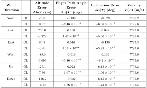
To evaluate performance, values of V , as well as errors in h, and i at the moment of insertion have been shown in Tables 2 and 3 for simulations of both OL and CL strategies. \Error" means dier-ence between desired and actual values. The target being a sun-synchronous orbit, the desired values for h(T ), (T ) and i(T ) are respectively, 200 km, 0 deg and 97.5 deg. In Tables 2 and 3, the wind speeds are, respectively, 6.5 m/s (known as a \moderate breeze" in the Beaufort scale) and 22 m/s (strong gale).

As the results indicate, if OL guidance is chosen, then, west-east winds can create great errors in param-eters values at the moment of orbit insertion. This is primarily due to the fact that the launch path is close to a polar orbit. Errors, particularly in i(T ) and (T ), are so large, the mission may be considered as failed for the OL case. The results also demonstrate the signicant improvement brought about by the CL algorithm at the cost, however, of a slightly lower speed at orbit insertion.

In reality, winds along down-up directions are seldom as strong as those in west-east or south-north directions. However, to see the eect of wind direction alone on guidance performance and for comparison

Table 2. Errors at the orbit insertion moment, T , for wind speed of 6.5 m/s. Wind

Direction

Altitude Error h(T ) (m)

Flight Path Angle Error (T ) (deg)

Inclination Error i(T ) (deg)

Velocity V (T ) (m/s) North OL -730 -0.136 -0.028 7798.2

CL 0.87 2:46 10 5 _{6:68 10} 6 _7795.6

South OL 730.0 0.136 0.028 7793.0 CL -0.929 1:47 10 5 _{5:60 10} 6 _7795.6

East OL 86.5 0.016 -0.130 7795.3 CL -0.44 4:16 10 6 _{5:89 10} 6 _7795.6

West OL -88.0 -0.016 0.130 7795.9 CL -0.099 3:40 10 6 _{6:1 10} 6 _7795.6

Up OL 126.1 0.022 6:15 10 6 _7795.2

CL 7.36 1:67 10 4 _{1:06 10} 6 _7795.6

Down OL -126.2 -0.022 6:15 10 6 _7795.9

purposes, down-up winds in simulations were taken to be as strong as those in other directions. A rst conclusion is that, even for OL guidance, the errors caused by down-up winds are not as large as those caused by west-east or south-north directions. Another conclusion is that CL guidance does succeed in signicantly reducing errors.

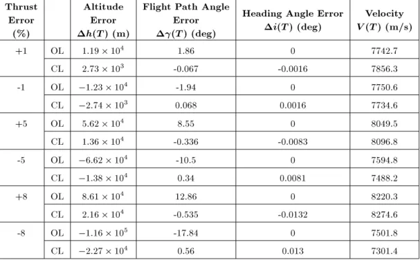
The thrust magnitude of each stage is assumed

to be within a few percent of its nominal value. Table 4 shows the eects of thrust magnitude (static) deviations on the accuracy of orbit insertion. For OL guidance, the error in i(T ) is not so great, however, the error in (T ) is large enough for the OL guidance to be considered as failed. In this case, too, the CL guidance algorithm greatly reduces the errors caused by thrust magnitude deviations.

Table 3. Errors at the orbit insertion moment, T , for wind speed of 22 m/s. Wind

Direction

Altitude Error h(T ) (m)

Flight path angle Error (T ) (deg)

Inclination Error i(T ) (deg)

Velocity V (T ) (m/s) North OL -8.91 103 _{-1.64 -0.33 7827.1}

CL 9.25 2:08 10 4 _{1:17 10} 5 _7795.5

South OL 8:97 103 _{1.70 0.36 7763.6}

CL -12.85 2:75 10 4 _{1:52 10} 6 _7795.4

East OL 956.9 0.179 -1.60 7792.1 CL -42.1 9:16 10 4 _{1:90 10} 5 _7793.1

West OL 1:18 103 _{-0.22 1.58 7799.8}

CL -37.7 8:20 10 4 _{1:63 10} 6 _7793.2

Up OL 1:54 103 _{0.273 6:13 10} 6 _7791.4

CL 90.11 -0.002 6:0 10 5 _7794.1

Down OL 1:55 103 _{-0.275 6:16 10} 6 _7799.8

CL -90.79 0.002 4:81 10 5 _7795.1

Table 4. Errors at the orbit insertion moment, T , caused by thrust magnitude error. Thrust

Error (%)

Altitude Error h(T ) (m)

Flight Path Angle Error (T ) (deg)

Heading Angle Error i(T ) (deg)

Velocity V (T ) (m/s) +1 OL 1:19 104 _{1.86 0 7742.7}

CL 2:73 103 _{-0.067 -0.0016 7856.3}

-1 OL 1:23 104 _{-1.94 0 7750.6}

CL 2:74 103 _{0.068 0.0016 7734.6}

+5 OL 5:62 104 _{8.55 0 8049.5}

CL 1:36 104 _{-0.336 -0.0083 8096.8}

-5 OL 6:62 104 _{-10.5 0 7594.8}

CL 1:38 104 _{0.34 0.0081 7488.2}

+8 OL 8:61 104 _{12.86 0 8220.3}

CL 2:16 104 _{-0.535 -0.0132 8274.6}

-8 OL 1:16 105 _{-17.84 0 7501.8}

To consider a more realistic scenario in the fol-lowing round of simulations, the thrust magnitude of each stage is 1% lower than its nominal value and the wind has components in west-east and south-north directions given, of course, by Equations 36 and 37, with E0 = N0= p15₂ = 10:61 m/s (a moderate gale)

and E = N = 0:9. The results are exhibited in

Figures 3 to 12. Solid, dashed and solid-dashed graphs in each gure correspond to CL, OL and purely nominal simulations, respectively.

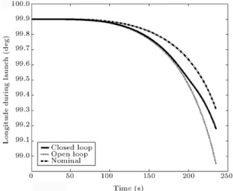
Figures 3 to 7 show graphs versus time t of the state-variables (t) (longitude), (t) (latitude), h(t) (altitude), (t) (ight-path angle) and (t) (heading angle) during the launch, i.e. for t0 t T .

Figures 8 and 9 show the graphs versus t of control variables (t) (angle of attack) and (t) (velocity-roll angle), again for t0 t T . Clearly, (t)

and (t) are identically zero in OL simulations, and near zero during the endoatmospheric phase of CL

Figure 3. Longitude during launch.

Figure 4. Latitude during launch.

simulations. However, (t) and (t) do take on large nonzero values during the exoatmospheric phase of CL simulations in order to eect guidance toward the target orbit.

The amplitude of variations in (t) and (t) are about 40 deg and 30 deg, respectively, implying that

Figure 5. Altitude during launch.

Figure 6. Flight path angle during launch.

Figure 8. Angle of attack during launch.

Figure 9. Velocity roll angle during launch.

Figure 10. Inclination during launch.

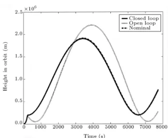
the vehicle may undergo intensive maneuvering. This, however, occurs outside the atmosphere and will not endanger the vehicle. Figure 10 depicts the variations of inclination i(t) during launch. Figures 11 and 12 show the latitude and velocity for a longer period of time, namely from lift-o to 7500 seconds after orbit

Figure 11. Altitude of satellite in orbit.

Figure 12. Velocity of satellite in orbit.

insertion. These gures make it possible to observe what happens to the satellite during one complete cycle around the Earth after insertion into the target orbit. The performance of the proposed guidance algorithm may be further veried by comparing the CL and OL graphs as follows. For the OL graphs, it can be seen from Figures 10 and 11 that i 101:7 deg instead of 97.5 deg, and jhjmin 50 km, which means

that the satellite will return to the atmosphere and eventually fall. For the CL graphs, on the other hand, one obtains i(T ) 97:5 deg, jhjmin 200 km from

the same gures. Furthermore, in the OL graphs, (T) 4 deg, implying a failed launch, while in the CL case, (T ) 0:01 deg which is an acceptable error. CONCLUSION

A guidance algorithm for sending a small satellite to a sun synchronous LEO was devised with the aims of simplicity of onboard computations and accuracy of orbit insertion. The onboard computations involve

no more than multiplying at each sampling time a 2 7 gain matrix by a 7 1 data vector. The gain matrices are computed o-line and stored in the onboard computer. Data are obtained through onboard measurements. The proposed algorithm performs accu-rate orbit insertion against wind disturbances of speeds of at least 22 m/s and thrust magnitude errors of at least 5%. Extending the method to launches to non-LEO environments or to other orbits can be subjects for future research.

NOMENCLATURE

a speed of sound

a LTL parameter in Equation 28 b LTL parameter in Equation 28 ci mass burning rate of the ith stage

f a function representing dynamics g gravitational acceleration

h altitude from sea level h1 air density constant

h2 air pressure constant

m mass

n random process

n disturbance vector

p air pressure

ps air pressure at sea level

q dynamic pressure

r distance from Earth center

t time

t0 launch start time

tv end of vertical launch time

u control vector

w wind force

x state vector

y output vector

z white random process

A see Equatuin 46

B see Equation 47

Ab aerodynamic reference area

Ae engine exit area of launch vehicle

AL lateral cross section area of launch

vehicle

CD drag coecient

CD0 drag coecient constant

CD1 drag coecient constant

CD2 drag coecient constant

CD3 drag coecient constant

CL lift coecient

CL1 lift coecient constant

CL2 lift coecient constant

D drag

F a function representing the nal output

L lift

M Mach number

M matrix relating output vector to state vector

Q scaling matrix

T thrust

T orbit insertion moment

Tvac thrust in vacuum

V velocity

Z denoting nominal values of state and control vectors

angle of attack

ratio of specic heat of air

ight path angle

see Equation 49

angle

longitude

velocity roll angle

wind speed

0 wind speed mean

air density

s air density at sea level

latitude

heading angle ! Earth rotating rate !p see Equation 26

dierence between actual and nominal value

Subscripts

nom nominal value

E east component

N north component

U up component

REFERENCES

1. Dubourg, V., Kainov, V., Thoby, M., Silkin, O. and Solovey, V. \The DEMETER micro satellite launch campaign: A cheap access to space", Advances in Space Research, 37, pp. 754-760 (2006).

2. Freeborn, P., Kinnersley, M. and Zorina, A. \The ROCKOT launch vehicle-the competitive launch so-lution for small Earth observation satellites into low Earth orbits", Acta Astronautica, 56, pp. 315-325 (2005).

3. Marrdonny, M. and Mobed, M. \A guidance algorithm for launch to equatorial orbit", Aircraft Engineering and Aerospace Technology, 81(2), pp. 137-148 (2009). 4. Sinha, S.K. and Shrivastava, S.K. \Optimal explicit guidance of multistage launch vehicle along three-dimensional trajectory", Journal of Guidance, Control and Dynamics, 13(3), pp. 394-403 (1990).

5. Battin, R.H., An Introduction to the Mathematics and Methods of Astrodynamics, AIAA Education series, New York (1987).

6. Madeira, F. and Rios-Neto, A. \Guidance and control of a launch vehicle using a stochastic gradient projec-tion method", Automatica, 36, pp. 427-438 (2000). 7. Pamadi, B.N., Taylor, L.W. and Price, D.B. \Adaptive

guidance for an aero-assisted boost vehicle", Journal of Guidance, Control and Dynamics, 13(4), pp. 586-595 (1990).

8. Lu, P. \Nonlinear trajectory tracking guidance with application to a launch vehicle", Journal of Guidance, Control and Dynamics, 19(1), pp. 99-106 (1996). 9. Lu, P., Sun, H. and Tsai, B. \Closed-loop

endoat-mospheric ascent guidance", Journal of Guidance, Control and Dynamics, 26(2), pp. 283-294 (2003). 10. Wiesel, W.E., Spaceight Dynamics, McGraw-Hill,

Singapore (1997).

11. Pamadi, B.N. \Simple guidance method for single stage to low earth orbit", Journal of Guidance, Control and Dynamics, 18(6), pp. 1420-1426 (1995).

12. Gralin, M.H., Telaar, J. and Schottle, U.M. \As-cent and reentry guidance concept based on NLP-methods", Acta Astronautica, 55, pp. 461-471 (2004). 13. Feeley, T.S. and Speyer, J.L. \Techniques for develop-ing approximate optimal advanced launch system guid-ance", Journal of Guidance, Control and Dynamics, 17(5), pp. 889-896 (1994).

14. Seywald, H. and Cli, E.M. \Neighboring optimal control based feedback law for the advanced launch system", Journal of Guidance, Control and Dynamics, 17(6), pp. 1154-1162 (1994).

15. Calise, A.J., Melamed, N. and Lee, S. \Design and evaluation of a three-dimensional optimal ascent

guid-ance algorithm", Journal of Guidguid-ance, Control and Dynamics, 21(6), pp. 865-875 (1998).

16. Leung, M.S.K. and Calise, A.J. \Hybrid approach to near-optimal launch vehicle guidance", Journal of Guidance, Control and Dynamics, 17(5), pp. 881-888 (1994).

17. Gath, P.F. and Calise, A.J. \Optimization of launch vehicle ascent trajectories with path constraints and coast arcs", Journal of Guidance, Control and Dynam-ics, 24(2), pp. 296-304 (2001).

18. Park, S. \Launch vehicle trajectories with a dynamic pressure constraint", Journal of Spacecraft and Rock-ets, 35(6), pp. 765-773 (1998).

19. Shaver, D.A. and Hull, D.G. \Advanced launch sys-tem trajectory optimization using suboptimal control", Proceedings of the AIAA Guidance, Navigation, and Control Conference, AIAA, Washington, DC (AIAA Paper 90-3413), pp. 892-901 (1990).

BIOGRAPHIES

Mohammad Marrdonny was born in 1975 in Iran. He received his Ph.D. from the Department of Elec-trical Engineering at Sharif University of Technology (S.U.T), Tehran in 2009, where he also received his B.S. and M.S. degrees in Electronics and Control Engineering in 1998 and 2000, respectively. His eld of interest is: Navigation and Guidance of Aerospace Vehicles.

Mohammad Mobed was born in 1954 in Iran. He received his B.S. degree from Sharif University of Technology, and his M.S. and Ph.D. degrees from The University of Michigan, Ann Arbor, all in Electrical Engineering in 1977, 1979 and 1988, respectively. He was a researcher and an instructor at the Iran Telecom-munications Research Center, Amirkabir University of Technology, and Tafresh University, during the period from 1994 to 1996. He has been with the Electrical En-gineering Department, Sharif University of Technology, as an Assistant Professor since 1997. His interests are in Systems aspects of Communications and Control.