A Hybrid Scatter Search for the RCPSP
M. Ranjbar
1;and F. Kianfar
2Abstract. In this paper, a new hybrid metaheuristic algorithm based on the scatter search approach is developed to solve the well-known resource-constrained project scheduling problem. This algorithm combines two solutions from scatter search to build a set of precedence feasible activity lists and select some of them as children for the new population. We use the idea presented in the iN forward/backward improvement technique to dene two types of schedule, direct and reverse, and the members of the sequential populations change alternately between these two types of schedule. Extensive computational tests were performed on standard benchmark datasets and the results are compared with the best available results. Comparative computational tests indicate that our procedure is a very eective metaheuristic algorithm.
Keywords: Project scheduling; Metaheuristic; Scatter search.
INTRODUCTION
The Resource-Constrained Project Scheduling Problem (RCPSP) is one of the most intractable optimization problems in operations research. Also, Blazewicz et al. [1] proved that the RCPSP, as a generalization of the job shop scheduling problem, is strongly NP-hard such that the computation times for obtaining the optimal solution using exact algorithms can be extremely high for more than 30 activities [2].
During previous decades, numerous exact, heuris-tic and metaheurisheuris-tic algorithms have been developed for this problem. There are several survey papers on the RCPSP and we mention here only some of the most recent ones. Herroelen et al. [3] surveyed the various branch-and-bound algorithms for the RCPSP. Kolisch and Hartmann [4] presented a classication and performance evaluation of dierent heuristic and meta-heuristic algorithms, including the recent advances in this eld. For an excellent survey and introduction of the RCPSP, we refer the readers to Demeulemeester and Herroelen [1].
Several exact solution approaches have been pro-posed for this problem: The linear programming based
1. Faculty of Engineering, Ferdowsi University of Mashhad, Mashhad, P.O. Box 91775-1111, Iran.
2. Department of Industrial Engineering, Sharif University of Technology, Tehran, Iran.
*. Corresponding author. E-mail: m [email protected] Received 7 April 2007; received in revised form 7 August 2007; accepted 22 September 2007
approach of Mingozzi et al. [5], the depth-rst branch-and-bound with dominance rules of Demeulemeester and Herroelen [6,7] and also the branch-and-bound algorithm of Brucker et al. [8], whose branching scheme uses a set of conjunctions and disjunctions to pairs of activities, are among some of the more eective exact procedures. In the heuristic approaches category, there are many dierent solution procedures, such as X-path methods [4], insertion techniques, based on the parallel scheduling generation scheme, and the worst case slack priority rule of Artigues et al. [9], the heuristic of Mohring et al. [10], based on Lagrangian relaxation and minimum cut computations, the network decom-position technique of Sprecher [11], which incorporates exact methodologies into a heuristic search, and the forward-backward improvement method of Tormos and Lova [12]. The metaheuristics include the genetic algorithm, simulated annealing, ant colony optimiza-tion, the tabu search, the scatter search, path relink-ing and hybrid algorithms. The algorithm of Valls et al. [13], which incorporates the genetic algorithm with the forward-backward-improvement method, is ranked the best hybrid metaheuristic algorithm to date. The genetic algorithm had been also used by Alcarez and Maroto [14], Hartmann [15,16] and Coelho and Tavares [17]. Bouleimen and Lecocq [18] tackle the RCPSP by means of simulated annealing, whereas Merkle et al. [19] use ant colony optimization. Nonobe and Ibaraki [20] suggest a tabu search for a generalized variant of the RCPSP. Also, Debels et al. [21] develop a hybrid metaheuristic, in which two elements from
scat-ter search are combined with a heuristic optimization method that simulates the electromagnetism theory of physics.
In this paper, we present a new hybrid meta-heuristic algorithm for the RCPSP based on the scat-ter search, further referred to as the Hybrid Scatscat-ter Search (HSS). Although it is a little similar to the scatter search presented in [21], it diers, particu-larly in terms of a combination method, the core of the scatter search and, also, in the use of the forward-backward-improvement method. In [21], a solution combination method is used based on the electromagnetism theory of physics, but we develop a solution combination method based on path relinking, in which a set of precedence feasible activity lists is generated, a number of which are selected as children by a specied procedure, as explained in the following sections. Furthermore, Debels et al. [21] use directly the forward/backward improvement technique as a local search (intensication method), but we use it in a dierent approach. We dene two kinds of schedule, direct and reverse schedules, using the idea introduced by Li and Willis [22], to employ some of the benets of their forward-backward improvement local search, but without performing a local search. In our HSS algorithm, the populations alternate sequentially between direct and reverse schedules.
The remainder of the paper is organized as fol-lows. First, denitions are provided. Then, the scatter search and the combination method for the RCPSP are presented. After that, the detailed and compara-tive performance tests on the benchmark datasets are described, and nally, the conclusions of this study are given.
DEFINITIONS Problem Denition
The RCPSP can be stated as follows. A single project consisting of a set, N, of activities, including n real activities and two dummy activities as the start and nish of the project, numbered from 0 to n + 1, has to be scheduled on a set, R, of constrained renewable resource types subject to nish-start-type precedence constraints with a time lag of zero. While being processed, activity i requires rik2 IN units of resource
type k 2 R in every time unit of its deterministic and non-preemptive duration, di 2 IN. The capacity of
resource k is constant throughout the project horizon and limited to Rk. The dummy start and nish
activ-ities have zero duration and resource usage, while the real activities have positive duration and nonnegative resource usage subject to rik Rk, i 2 N, k 2 R. The
objective of RCPSP is to nd a precedence and resource feasible schedule, S, dened by a nish time vector,
f = (f0; ; fn+1), such that the project makespan,
fn+1, is minimized.
Schedule Representation
Our constructive heuristic algorithm relies on a Sched-ule Generation Scheme (SGS) and schedSched-ule represen-tation. The schedule generation scheme determines the way in which a feasible schedule is constructed by assigning starting or nishing times to the dierent activities and the schedule representation is a repre-sentation of a relative priority rule determining the activity that is selected next during the scheduling process.
We work with the serial SGS, since it generates active schedules [23]. Active schedules contain optimal schedules if the measure of performance is regular and the makespan is a regular measure of performance. In each iteration of the serial SGS, the activity with the highest priority is chosen and assigned the rst possible starting time, such that no precedence or resource constraint is violated. Also, we choose to use the Activity List (AL) representations, since it is one of the most commonly used schedule representations in the development of heuristics for the RCPSP [24]. Each AL is a sequence of activities, in which the position of each activity in the sequence determines its relative priority versus the other activities.
Direct and Reverse Schedule
For dening direct and reverse schedules, we rst dene a direct and reverse project network. The direct project network is a network in which the arrows show the original precedence relations. If the directions of all the arrows are reversed, the resulting network is dened as the reverse project network. Now, any feasible schedule for the direct network is called a direct schedule and any feasible schedule for the reverse project network is called a reverse schedule.
Precedence Feasible and Topologically Ordered Activity List
As dened, AL may not be precedence feasible. If an AL is precedence feasible, we call it the Precedence Feasible Activity List (PFAL), in which every activity is positioned after all of its predecessors. To obtain the precedence feasible activity list, which has a Topologi-cal Order-condition (TO-condition), we have to sched-ule the activities and then order them based on their topological position, called topological ordering. In the original denition of the TO-condition introduced by Valls et al. [25] for direct schedules, for all i and j, if the start time of activity i is smaller than the start time of activity j, activity i should have a higher
priority than activity j. We adapted the TO-condition to our settings for two types of schedule; direct and reverse. More precisely, HSS uses direct schedules to generate reverse children and reverse schedules to generate direct children. To embed the TO-condition in the AL-representation, we rst schedule the activities using the serial SGS and a given AL and, then, we sort the activities based on the non-increasing order of their nish times, i.e. for all i and j, if fi(S) > fj(S),
activity i should have a higher priority than activity j. The result of applying the TO-condition on an arbitrary AL is a Topologically Ordered Activity List shown as TOAL. The dierence between the denition of the TO-condition in our settings and the original one is due to the use of two types of schedule; direct and reverse schedules, in our algorithm.
THE HYBRID SCATTER SEARCH ALGORITHM
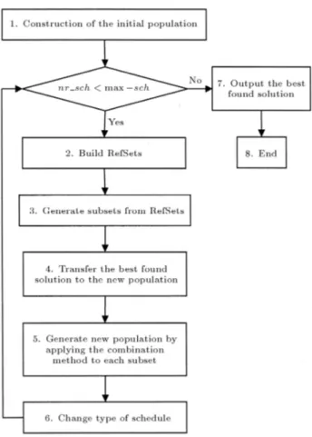
Our algorithm is based on scatter search, an evolution-ary method that constructs new solutions by combining existing ones in a systematic way. For details of SS, we refer the readers to Marti et al. [26]. The steps of our HSS are depicted in Figure 1 and explained below.
Figure 1. Flowchart of the hybrid scatter search algorithm.
Construction of the Initial Population
In the rst step, we generate an initial population (P ) of TOALs with size jP j. Each TOAL in the initial population is obtained from a direct schedule applied on a randomly generated AL using the serial SGS. Construction of the New Population
Steps 2, 3, 4, 5 and 6 of the algorithm, shown in Figure 1, are used to generate the new population. In the second step, we build a reference set (RefSet) consisting of RefSet1 and RefSet2. RefSet1 is a set of
size b1 of TOALs with the least makespans, selected
from the current population. Every TOAL of RefSet1
should have a distance more than t1with other TOALs
of RefSet1. The distance of two TOALs, say TOAL1
and TOAL2, is computed as follows [21]:
distance (TOAL1; TOAL2)
= n1
n
X
i=1
jposition of activity i in TOAL1
position of activity i in TOAL2j:
Due to distance threshold t1, there may not be enough
TOAL in the current population to make a complete RefSet1. In this case, the rest of the needed TOALs for
RefSet1 are generated randomly, as explained for the
initial population, and they are not tested for having minimum distance t1 with other elements of RefSet1.
RefSet2 has the size of b2 TOALs selected from P n
RefSet1, in the same way as explained for RefSet1, but
the distance of each selected element should be more than t2, t2> t1, from each element of RefSet1and other
elements of RefSet2. If needed, random generation
of TOALs is used for RefSet2 too. The distance
thresholds, t1 and t2, are imposed to RefSet1 and
RefSet2, respectively, in order to avoid homogeneous
solutions and keep diversity in each population. The solutions in the RefSet1 and RefSet2 are ordered,
according to their quality.
In Step 3, we select solutions from RefSet1 and
RefSet2to be combined. For this purpose, we generate
two-element subsets of either two solutions in RefSet1
or one from RefSet1and one from RefSet2, respectively,
resulting in
b1
2
+ b1 b2 subsets. Before starting
the combination phase, we add the best found solution to the new population in Step 4. Next, the elements of each subset are combined using the combination method, which will be described later, in order to generate the new population. From each combination, a set of PFALs is generated and then nrc of them are selected by a systematic random selection as the
combination children. These children are incorporated with the TO-condition and then added to the new pop-ulation. Based on our denition of the TO-condition, the direct schedules generate reverse children and the reverse schedules generate direct children. By applying the combination method to the elements of all subsets and adding the best so far solution, we obtain a new population with size
b1
2
+ b1 b2
nrc + 1 that remains constant for all populations. In Step 6, we change the type of schedule from direct to reverse or vice versa. The termination criterion is considered as the maximum number of generated schedules and denoted as max sch, which is in line with the existing literature on the RCPSP heuristics. Steps 2 to 6 are repeated until the number of generated schedules (nr sch) is smaller than max sch. Step 7 selects the best solution in the population as the output of the algorithm.
Combination Method
In Step 5 of Figure 1, we use our combination method to generate nrc children from each subset generated in Step 3 of the scatter search algorithm. In our combination method, we make use of the path relinking idea, originally proposed by Glover and Laguna [27]. This method explores a set of PFALs obtained by moving between the two elements of each subset. Since each TOAL is also a PFAL, and we consider only the precedence feasibility in the combination method, we call these two elements the guiding and initial PFAL, denoted as PFAL1 and PFAL2, respectively.
The PFAL1 and PFAL2 are specied, such that the
makespan of PFAL1is not worse than the makespan of
PFAL2 and the move direction is always from PFAL2
towards PFAL1. To explain the combination method,
we rst consider the following process. Suppose we have a precedence feasible activity list denoted as PFAL = (0; [1]; ; [n]; n + 1), in which [p] represents the activity located at position p in PFAL. If we exchange activities [p] and [q], q > p, we get a new activity list, which may not be precedence feasible. Suppose we know that activity [q] in position p is precedence feasible and we are looking for a PFAL which has activity [q] in position p. For this purpose, we start from position p + 1 and move to the right of PFAL and, at each position, say position y, if the activity at position q of the current list is the predecessor of activity [y], we exchange the activities in positions y and q. This move is continued till y = q and we get the desired PFAL.
Now, the combination method can be ex-plained. Let the guiding PFAL be PFAL1 =
(0; [1]1; ; [n]1; n + 1) and the initial PFAL be
PFAL2 = (0; [1]2; ; [n]2; n + 1). First, we make a
set, C, of precedence feasible activity lists as follows: we nd the smallest p, for which [p]16= [p]2and assume
activity [p]1 is located at position q of PFAL2, i.e.
[q]2= [p]1. Note that q is larger than p. Now, in order
to have the same activity at position p in both PFAL1
and PFAL2, we exchange the activities in position p
and q of PFAL2 and call the resulting list AL. If AL is
precedence feasible, it is added to set C; otherwise, we change it to a PFAL, as explained above, and then add it to set C. Note that the added PFAL has the same ac-tivities as PFAL1in positions 1 to p. Now, consider this
PFAL as the PFAL2 and repeat the process till p = n.
At this point, we have jCj precedence feasible activity lists, whose characteristics changed progressively from the characteristics of the initial PFAL to that of the guiding PFAL. The combination of PFAL1and PFAL2
terminates by selecting nrc of PFALs from set C, using a systematic random sampling, as the children of them. To select nrc children from set C, we number its members from 1 to jCj and divide them as equally as possible to bjCj=nrcc subsets. Then, we select one member from each subset randomly. The selected children are incorporated with the TO-condition and then added to the new population.
A Numerical Example
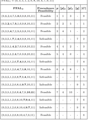
Figure 2 represents an example project and Figure 3 illustrates the combination method. In this project, there is only one constrained renewable resource with 4 available units.
In the example shown in Figure 2, we have considered PFAL1= (0; 3; 5; 1; 2; 6; 8; 10; 4; 7; 9; 11) and
PFAL2 = (0; 1; 2; 4; 7; 5; 3; 6; 9; 8; 10; 11). In the rst
step, we have p = 1, where [1]1 6= [1]2 and, therefore,
activities [1]2 = 1 and [1]1 = 3 of PFAL2 should
be exchanged. The successor of activity 1 with the lowest position in the new activity list, AL, is activity 6 located at position 7; therefore, this new activity list is precedence feasible and is added to set C. Note
Figure 3. Illustration of the combination method.
that we consider this added list as the PFAL2 for
the next step. Follow the similar process in Step 2 for activities 2 and 5 in the new PFAL2. In the
third step, where activities 4 and 1 are exchanged, we obtain a precedence infeasible activity list, because the successor of activity 4 with the lowest position, activity 7, is located before activity 4, therefore, it should be exchanged with activity 4. As the successor of activity 7, with the lowest position in the new activity list, activity 9, which is located after activity 7, we have found a new PFAL, called PFAL2. By following
the combination procedure, set C will contain 6 new precedence feasible activity lists. Note that the rst and the last precedence feasible activity lists in Figure 3 are the PFAL2 and PFAL1, respectively, and are not
eligible to be considered as the members of set C. If we assume nrc = 2, we have to divide C to two subsets, C1 and C2, including the rst three and the
last three members of C. r1 = 2 and r2 = 1 are
two random numbers between 1 to 3, as the selected members from subsets C1 and C2, respectively, which
have been specied with the gray color in Figure 3. PERFORMANCE TESTS
We tested the performance of our HSS algorithm as explained below. The HSS procedure was coded in
Visual C++ 6.0 and the computer used was a PC Pentium IV 3GHz processor with 1024 Mbytes of RAM. The problem set was taken from PSPLIB datasets [28]. The dataset consists of four test sets J30, J60, J90 and J120 that contain problem instances of 30, 60, 90 and 120 activities, respectively, and have been constructed by the instance generator ProGen [29]. In this study, the maximum number of generated sched-ules (max sch) was considered as the termination criterion, in order to be able to compare the results of the proposed procedure with the results reported in the literature and be independent of the computer platform, compilers and implementation skills. This criterion holds, in particular, for methods which apply the serial or parallel SGS; one pass of an SGS, with one start time assignment per activity, counts as one schedule.
Before using the coded HSS for performance tests, we tuned the parameters of HSS. For nrc, we tested the values of 1, 2, 3, 4 and 5 and noted that nrc = 2 gives the best results and is not sensitive to the values of the other parameters, hence, it was xed at 2. The other parameters of HSS were tuned for each test set. The tuned values of the other parameters that have been obtained by ne tuning are presented in Table 1. This table reveals that the tuned values of the size of the initial population, jP j, and the size of RefSet1 and RefSet2, b1 and b2, are positively related
to max sch, while the tuned values of threshold distances, t1 and t2, are positively related to the
number of activities.
The details of the computational results are shown in Table 2. The rows labeled \Sum" give the sum of the makespans of all problem instances in each test set. The rows, labeled \Avg. Dev. CPM", represent the average percent deviation from the critical-path lower bound. The two next rows, labeled \Avg. Dev. Hrs" and \Avg. Dev. LB", indicate the average percent
Table 1. Tuned values of the parameters. Parameter max sch Data Set
J30 J60 J90 J120 t1 1 1 1 1.1
t2 1.9 2.1 2.2 2.3
1000 4 4 3 4 b1 5000 7 6 8 7
50,000 21 22 18 21 1000 2 4 2 2 b2 5000 7 5 4 5
50,000 13 15 17 14 1000 50
jP j 5000 100 50,000 500
Table 2. Detailed computational results. Problem Set max sch Data Set
J30 J60 J90 J120 1000 28352 38722 46297 76664 Sum 5000 28326 38541 46030 75612 50,000 28316 38395 45802 74620 1000 13.53% 11.59% 11.24% 35.08% Avg. Dev. CPM 5000 13.41% 11.07% 10.60% 33.24% 50,000 13.37% 10.64% 10.04% 31.49% 1000 0.10% 0.83% 1.21% 3.55% Avg. Dev. Hrs 5000 0.03% 0.47% 0.75% 2.36% 50,000 0.00% 0.17% 0.37% 1.24% 1000 0.10% 2.75% 3.06% 7.94% Avg. Dev. LB 5000 0.03% 2.37% 2.58% 6.66% 50,000 0.00% 2.05% 2.16% 5.46% Num. Test Problem 480 480 480 600
1000 453 362 361 194 Best 5000 471 384 369 215 50,000 480 416 389 252 Improved 50,000 - 0 5 18
1000 0.03 0.07 0.12 0.24 Avg. CPU (seconds) 5000 0.14 0.34 0.58 1.18 50,000 1.67 4.07 6.54 13.58
deviation from the currently best known solutions and best known lower bounds, respectively, based on PSPLIB results from January 1, 2007. The row labeled \Num. Test Problem" indicates the number of problem instances in each test set and the rows labeled \Best" show the number of instances for which our HSS algorithm reports a makespan not worse than the currently best known solution. The row labeled \Improved" reports the number of problem instances for which we have been able to improve the best known solution (it can be seen at PSPLIB) and the last rows labeled \Avg. CPU" indicate the average computation time per instance.
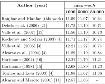
Comparative results are available for sets J30, J60 and J120 in the literature. Tables 3 to 5 display the rank of HSS among ten best heuristics, up to the current date for the test sets J30, J60, and J120, respectively, based on the results presented in the literature survey paper [4] and the new developed research paper [13]. The comparison is made for values of 1000, 5000 and 50000, as the limits of the maximum number of schedules. For the J30 set, the results are given in terms of average percent deviation from the makespan of the optimal solution. For the other sets, the average percent deviation from the
Table 3. Comparative results for J30. Author (year) max sch
1000 5000 50,000 Ranjbar and Kianfar (this work) 0.10 0.03 0.00 Kochetov and Stolyar (2003) [4] 0.10 0.04 0.00 Debels et al. (2006) [21] 0.27 0.11 0.01 Valls et al. (2007) [13] 0.27 0.06 0.02 Valls et al. (2005) [4] 0.34 0.20 0.02 Alcaraz et al. (2004) [4] 0.25 0.06 0.03 Alcaraz and Maroto (2001) [14] 0.33 0.12 -Tormos and Lova (2003) [4] 0.25 0.13 0.05 Nonobe and Ibaraki (2002) [20] 0.46 0.16 0.05 Tormos and Lova (2001) [12] 0.30 0.16 0.07
critical path-based lower bound is used as a measure of performance, since many optimal solutions are unknown. In all tables, the heuristics are sorted for the case of max sch = 50000. As a tie-breaker, the results for 5000 and then 1000 schedules are used in sorting. Tables 3 to 5 reveal that HSS outperforms other heuristic for J30 and J60 and is ranked second for J120.
Table 4. Comparative results for J60. Author (year) max sch
1000 5000 50,000 Ranjbar and Kianfar (this work) 11.59 11.07 10.64 Debels et al. (2006) [21] 11.73 11.10 10.71 Valls et al. (2007) [13] 11.56 11.10 10.73 Kochetov and Stolyar (2003) [4] 11.71 11.17 10.74 Valls et al. (2005) [4] 12.21 11.27 10.74 Alcaraz et al. (2004) [4] 11.89 11.19 10.84 Hartmann (2002) [16] 12.21 11.70 11.21 Hartmann (1998) [15] 12.68 11.89 11.23 Tormos and Lova (2003) [4] 11.88 11.62 11.36 Alcaraz and Maroto (2001) [14] 12.57 11.86
-Table 5. Comparative results for J120. Author (year) max sch
1000 5000 50,000 Valls et al. (2007) [13] 34.07 32.54 31.24 Ranjbar and Kianfar (this work) 35.08 33.24 31.49 Alcaraz et al. (2004) [4] 36.53 33.91 31.49 Debels et al. (2006) [21] 35.22 33.10 31.57 Valls et al. (2005) [4] 35.39 33.24 31.58 Kochetov and Stolyar (2003) [4] 34.74 33.36 32.06 Valls et al. (2005) [4] 35.18 34.02 32.18 Hartmann (2002) [16] 37.19 35.39 33.21 Tormos and Lova (2003) [4] 35.01 34.41 33.71 Merkle et al. (2002) [19] - 35.43
-SUMMARY AND CONCLUSIONS
In this paper, we presented a hybrid metaheuristic algorithm for solving the resource-constrained project scheduling problem. This algorithm contains a scatter search skeleton and uses a special solution combination method for making children. The performance of the algorithm has been tested on test sets J30, J60, J90 and J120 from PSPLIB. The comparative computa-tional results show that our procedure outperforms other state-of-the art heuristics in the literature for J30 and J60 and is the second-best for test set J120. We think that three factors are the cause of the high performance of our algorithm, namely the structure of our scatter search, the solution combination method and the generation of reverse schedules from direct schedules and vice versa. We chose the general structure of a scatter search but with a new solution combination method. In this method, we move in the space of the precedence feasible activity lists, which is much smaller than the space of all possible
activity lists. We move between promising solutions and try as much as possible to have the benets of explorations in the solution space. Furthermore, the forward-backward improvement technique, introduced by [22], has recently been used as a local search in many developed metaheuristics, but we used it in a dierent manner. We changed the population of solutions alternately from direct schedules to reverse schedules and vice versa, to exploit the benet of the forward-backward improvement technique.
For further research, we recommend the idea of this hybrid scatter search for solving other combinato-rial optimization problems.
REFERENCES
1. Blazewicz, J., Lenstra, J.K. and Rinnooy Kan, A.H.G. \Scheduling subject to resource constraints: classica-tion and complexity", Discrete Applied Mathematics, 5(1), pp. 11-24 (1983).
2. Demeulemeester, E. and Herroelen, W., Project Scheduling - A Research, Handbook, Boston, Kluwer Academic Publishers (2002).
3. Herroelen, W. and Demeulemeester, E. and De Reyck, B. \Resource-constrained project scheduling- A survey of recent developments", Computers and Operations Research, 25(4), pp. 279-302 (1998).
4. Kolisch, R. and Hartmann, S. \Experimental inves-tigation of heuristics for resource-constrained project scheduling: An update", European Journal of Opera-tional Research, 174(1), pp. 23-37 (2006).
5. Mingozzi, A., Maniezzo, V., Ricciardelli, S. and Bianco, L. \An exact algorithm for the resource-constrained project scheduling problem based on a new mathematical formulation", Management Science, 44(2), pp. 714-729 (1998).
6. Demeulemeester, E. and Herroelen, W. \A branch-and-bound procedure for the multiple resource-constrained project scheduling problems", Manage-ment Science, 38(1), pp. 1803-1818 (1992).
7. Demeulemeester, E. and Herroelen, W. \New bench-mark results for the resource-constrained project scheduling problem", Management Science, 43(1), pp. 1485-1492 (1997).
8. Brucker, P., Knust, S., Schoo, A. and Thiele, O. \A branch & bound algorithm for the resource-constrained project scheduling problem", European Journal of Operational Research, 107(2), pp. 272-288 (1998). 9. Artigues, C., Michelon, P. and Reusser, S. \Insertion
techniques for static and dynamic resource-constrained project scheduling", European Journal of Operational Research, 149(2), pp. 249-267 (2003).
10. M Ohring, R., Schulz, A., Stork, F. and Uetz, M. \Solving project scheduling problems by minimum cut computations", Management Science, 49(3), pp. 330-350 (2003).
11. Sprecher, A. \Network decomposition techniques for resource-constrained project scheduling", Journal of the Operational Research Society, 53(4), pp. 405-414 (2002).
12. Tormos, P. and Lova, A. \A competitive heuristic solution technique for resource-constrained project scheduling", Annals of Operations Research, 102(1), pp. 65-81 (2001).
13. Valls, V., Ballestin, F. and Quintanilla, M.S. \A hybrid genetic algorithm for the resource-constrained project scheduling problem", European Journal of Operational Research, 185(2), pp. 495-508 (2008).
14. Alcaraz, J. and Marot, C. \A robust genetic algorithm for resource allocation in project scheduling", Annals of Operations Research, 102(1), pp. 83-109 (2001). 15. Hartmann, S. \A competitive genetic algorithm for
resource-constrained project scheduling", Naval Re-search Logistics, 45(1), pp. 733-750 (1998).
16. Hartmann, S. \A self-adapting genetic algorithm for project scheduling under resource constraints", Naval Research Logistics, 49(3), pp. 433-448 (2002). 17. Coelho, J. and Tavares, L. \Comparative analysis of
metaheuristics for the resource constrained project scheduling problem", Technical Report, Department of Civil Engineering, Instituto Superior Tecnico, Portugal (2003).
18. Bouleimen, K. and Lecocq, H. \A new ecient simu-lated annealing algorithm for the resource-constrained project scheduling problem and its multiple modes version", European Journal of Operational Research, 149(2), pp. 268-281 (2003).
19. Merkle, D., Middendorf, M. and Schmeck, H. \Ant colony optimization for resource-constrained project scheduling", IEEE Transactions on Evolutionary Computation, 6(1), pp. 333-346 (2002).
20. Nonobe, K. and Ibaraki, T. \Formulation and tabu search algorithm for the resource constrained project scheduling problem", in Essays and Surveys in Meta-heuristics, C.C. Ribeiro and P. Hansen, Eds., Kluwer Academic Publishers, pp. 557-588 (2002).
21. Debels, D., De Reyck, B., Leus, R. and Vanhoucke, M. \A hybrid scatter search/electromagnetism meta-heuristic for project scheduling", European Journal of Operational Research, 169(2), pp. 638-653 (2006). 22. Li, K.Y. and Willis, R.J. \An iterative scheduling
technique for resource-constrained project scheduling", European Journal of Operational Research, 56(8), pp. 370-379 (1991).
23. Kolisch, R. \Serial and parallel resource-constrained project scheduling methods revisited: Theory and computation", European Journal of Operational Re-search, 90(2), pp. 320-333 (1996).
24. Kolisch, R. and Hartmann, S. \Heuristic algorithms for solving the resource-constrained project scheduling problem: Classication and computational analysis", in Project Scheduling: Recent Models, Algorithms and Applications, J. Weglarz, Ed., Berlin, Kluwer Aca-demic Publishers, pp. 147-178 (1999).
25. Valls, V., Quintanilla, M.S. and Ballestin, F. \Resource-constrained project scheduling: A critical reordering heuristic", European Journal of Operational Research, 149(2), pp. 282-301 (2003).
26. Marti, R., Laguna, M. and Glover, F. \Principle of scatter search", European Journal of Operational Research, 169(2), pp 359-372 (2006).
27. Glover, F. and Laguna, M. \Tabu search", in Modern Heuristic Techniques for Combinatorial Problems, C. Reeves, Ed., Oxford, Blackwell Scientic Publishing, pp. 70-141 (1993).
28. Kolisch, R. and Sprecher, A. \PSPLIB - A project scheduling library", European Journal of Operational Research, 96(1), pp. 205-216 (1997).
29. Kolisch, R., Sprecher, A. and Drexl, A. \Character-ization and generation of a general class of resource-constrained project scheduling problems", Manage-ment Science, 41(10), pp. 1693-1703 (1995).