AUTOMATIC SPOKEN LANGUAGE RECOGNITION FOR MULTILINGUAL SPEECH RESOURCES

8379

AN EFFICIENT HYBRID MODEL FOR RELIABLE

CLASSIFICATION OF HIGH DIMENSIONAL DATA USING

K-MEANS CLUSTERING AND BAGGING ENSEMBLE

CLASSIFIER

1_{HAYDER K. FATLAWI} 2_{ABBAS F. H. ALHARAN} 3_{NABEEL SALIH ALI*}

1,3 _{Information Technology Research and Development Center, University of Kufa, Iraq.}

2_{Computer Department, College of Education for Girls, University of Kufa, Iraq.}

1_{[email protected],} 2_{[email protected],} 3_{[email protected]} 

ABSTRACT

Data mining is playing a significant role in the digital era, and there are traditional techniques to classify, cluster the large data, etc. Today, the variety of data and its size has grown increasingly. Preprocessing of the data impose and need high computational resources due to raising the number of data attributes. Thus, attributes reduction deem a vital and significant part of the data pre-processing due to its ability to reduce the required computational resources. In this study, a hybrid model is proposed to eliminate irrelevant attributes with N number of goodness evaluation metrics by using K-Means Clustering and Bagging Ensemble Classifier. The proposed model was implanted with five different datasets. The model can minimize the number of the attributes up to (70%). Hence, the results with reduction can be increased the efficiency of the classification performance from the computation time standpoint.

Keywords:k-means clustering, Bagging classification, Attributes reduction.

1.INTRODUCTION

Data mining concerns with discovering the hidden patterns and predicting unknown values in a large amount of data [1, 2]. Techniques of data mining have been increased attention by researchers due to raises the need for large and complex data analysis [3]. According to digital universe statistics, the approximate size of the data in 2005 was 130 Exabytes and is expected to reach 40,000 Exabytes, with increasing factor 300[4]. The high dimensionality of data (i.e., the large number of attributes in data) represents a significant challenge faces data mining techniques, whereas, the increasing of attributes lead to dramatically increase in the required computing resourced [5].

On the other hands, most solutions to this challenge focused on reducing the attributes by choosing the most correlated attributes with the target of classification (or removing the most irrelative attributes) [1,6,7]. The importance of an attribute can be determined using some statistical metrics, and the selection of the most suitable parameter represents another challenge [1, 2, 6]. The difficulty of this challenge increases when several metrics are used.

In the current work, a hybrid and multi-stage model is proposed to solve the mentioned challenges due to the ability to deal with any number of metrics to minimize the attributes. The model uses a K-means clustering algorithm to discover the strength patterns of the attributes. Then, reduced the data is classified using bagging ensemble techniques to improve the accuracy of the classification.

2.LITERATURE REVIEW

Attribute selection is a method that used to eliminate undesirable and recurrent attributes from data during processing. Overlooking the un-meaningful attributes from the enormous database minimizes the complexity and time of computation, and maximizes the quality of learning [8]. Two main categories of attribute selection methods are used which are supervised and unsupervised [9]. Diverse attempts by authors are introduced unsupervised selection methods to eliminate undesirable and recurrent data attributes.

8380 classification while both accuracy and detection of four categories are increased when implemented the proposed method in the KDD CUP 99 dataset.

Besides, an attributes selection method introduced by [11]. The method combining multivariate filter model with ant colony optimization (ACO) algorithm. The selection method was produced precise results after tested via new heuristic measurement.

On the other hands, in the field of text mining, as stated in [12], both clustering and classification based selection attributes have experimented. The authors applied hierarchical clustering (hClust) and k-means clustering with various lengths (5%), (10%), (15%), (20%) and (50%). Using a genetic algorithm of the selected attributes. Two measured are used with results which are average accuracy and F-measure to evaluate the performance of hClust and compare with k-means. The results found the performance of the hClust better than K-means when the length of attributes equal to or greater than (15%).

A hybridization approach of SVR, SOFM, and filter based attribute selection have been introduced by [13] to improve the accuracy of prediction for next day price index. SVR model is constructed for each cluster generated by SOFM according to select attributes. The result proved that the proposed approach better than using only SVR with and without attribute selection.

Also, an unsupervised method for attribute selection is presented by [14]. This method is based on the salient attribute selection by discovering the nearest neighbor and farthest neighbor (FSNF) to be held for clustering (k-means and SOM). Furthermore, filter-based and wrapper-based selection methods are discussed and compared with the proposed method to demonstrate the results. Whereas the filter-based method includes three models (Max-Rel, Var. and IBNF); whilst, the wrapper-based method k-means clustering algorithm is used in the training side.

As alongside with [15] which authors proposed another unsupervised attribute selection method that depends on availing the self-representation capability of attributes. Moreover, the representative attributes matric is influenced by itself to construct regularized attributes. The discordant is reduced by using L1, 2-norm, where the selected attributes are the most affection to construct other attributes. The presented method is evaluated by three criteria classification performance, clustering performance, and the redundancy.

Likewise, [16] proposed an approach to predict early failures detection in the air pressure system of

the trunks (Scania) to reduce the cost of the maintenance process. The conducted approach used the random forest to predict the classes of features (created as histograms), and it calculates the value of each class. Data (includes 60000 rows and 171 columns) has been used for training and evaluating the performance of the discussed approach. The results prove that the product approach has reduced the main cost around (0.6) compared to the traditional case (without approach).

Furthermore, Auto-Associative Multivariate

Regression Trees (AAMRT) approach is presented by [17] for unsupervised feature selection to preserve information and reduce data. The AAMRT based on multivariate regression tree (MRT) but the original variables in AAMRT are utilized as response and explanatory variables. Besides, the approach described the MRT and Classification and Regression Trees (CART). Several experiments are applied to different datasets such as Synthetic, Viruses, Flavour, viruses and Bacteria to evaluate The AAMRT approach. The proposed method is effective in selecting and maintaining the important features and expelling the frequent and unimportant features based on their evaluation results.

Moreover, fast feature selection method based on clustering (FAST) is proposed by [18]. The proposed method includes two steps respectively, First: using a graph-theoretic clustering method to divide the attributes into clusters. Second: create the subset of attributes from collecting the most related attributes to a particular class. The Fast method has experimented on 35 datasets with different domains to measure its performance. From the feature selection effectiveness end, FAST results in the best ratio (1.18%) of attribute selection compared with five algorithms namely: FCBF, CFS, Relief, Consist, and FOCUS-SF. Also, the FAST is the faster in running with time 3573 millisecond. Besides, the outcomes of the experiment that FAST produces smaller subsets and improves the accuracy of other classifiers such as Naive Bayes, C4.5, IB1, and RIPPER.

3.METHODOLOGY

8381

3.1Attributes Goodness Evaluation

One of the most critical decisions that should be taken during classification model growing is which attribute is most suitable for splitting data? [2]. Also, the question about which is the most suitable splitting value takes a significant role in this process? [1]. Wherefore, the reduction of many attributes leads to an effective decreasing in computing recourses [5]. For more confident elimination of attributes, the evaluation of attributes quality should depend on several metrics. Each

measurement could be ranked the attributes differently from the other measure which represents another challenge to be solved.

In this step, k metrics can be applied to the raw data to evaluate the quality of the attributes. Typical and straightforward rule classification method is used to perform the measurement. With N number of attributes, the result of this step is N × K matrix contains the quality of every attribute according to all metrics, such that element i in the matrix represents the goodness of attribute N_i using K_i criterion. This matrix would be used as an input for the next step.

3.2Attributes Clustering using K-means

8382

3.3Irrelevant Attributes Removal

According to the distribution of the attributes into two clusters, the decision will be taken to remove the

subset of attributes that belong to the weak cluster. The weakness of the cluster is detected by comparing the values of the center elements of the two clusters and the cluster with the lowest values in its center that will be considered the weak cluster. Thereby, all attributes in the weak cluster will be recovered due to the irrelevant to the target in the next classification process.

3.4Bagging Classification

Instead of creating one single classification model as a result of the training process, an ensemble classifier is created based on the bagging method [2, 6, 21]. Given the reduced dataset DS which contains m attributes and n rows the training include k iterations and for iteration (i<=k), DSi is a randomly sampled subset from DS with replacement. The training process on DSi produces a classification model CMi that could be applied to classify unseen data rows. The ensemble classifier collects the votes from each single classification model CMi and assigns the class with the highest number of votes to the hidden data [20- 24].

4.IMPLEMENTATION AND RESULTS

The implementation includes applying all steps of the proposed model with a sundry and different dataset. Evaluation of classifier’s performance is performed by using five accuracy metrics inanition with computational time metric.

4.1Description of Datasets

In the current study, five different datasets from a variety and diverse fields are used to apply and evaluate the proposed model as follow: (1) bank marketing dataset which depends on phone calls, it contains (17) attributes and (45211) data rows [25]. (2) Diabetes dataset contains clinical care data of 130 US hospitals for ten years (1999-2008), there are (50) attributes and (100000) data rows including in this dataset [26]. (3) MoCap hand postures contain data of 12 users with five different types of hand postures which collected using unlabeled markers, the total number of data rows of this dataset is (78095) and (38) attributes [27, 28]. (4) KDD Cup dataset of the third international competition of knowledge discovery and data mining tools, its task was to develop a network intrusion detector to

distinguish between intrusions and standard connections. It contains (42) attributes and (4000000) data rows [29]. (5) APS Failure at Scania Trucks includes (60000) data rows and (171) attributes; also it has two classes: positive class represents failures APS system component and negative level for failures for not related APS components [30].

4.2Applying Attributes Goodness Evaluation One of the most critical issues during the growth of a classifier is evaluating of attribute’s importance [2, 6]. In each division of the data process, the most relevant attribute with the target of the classification must be chosen. Statistical measures could be used for this task such as Information Gain and Gain Ratio [1, 2]. The best attribute is such an attribute that minimizes the impurity of data. Impurity could be measured using statistical randomness measurement such us Entropy. Therefore, Information Gain is the gain of splitting operation indicates by the impurity of the class Y before and after splitting [2]. The equation (1) explains the calculation of information gain as follow,

𝐈𝐧𝐟𝐨. 𝐆𝐚𝐢𝐧 𝑰𝒏𝑮 𝑷 ∑𝒄𝒏 𝑵𝑫 𝒏𝒐𝒅𝒆 𝒊_𝑵𝑫

𝒊 𝟏 𝑰𝒏𝑮 𝒏𝒐𝒅𝒆 𝒊

(……… (1)

where InG (P) is the parent node’s information gain before splitting, cn is the number of attribute‘s values, ND is the number of data row in the parent node, ND (node i) is the number of data row in node I, InG (node i) is the information gain of node i. The impurity of data is measured by Information Gain depending on the entropy which tends to select attributes with distinct high values. A high number of values led to generate more branches in each iteration. As a result of that; the number of data rows would be decreased which affects the prediction reliability. Gain Ratio represents an improvement to overcome this problem which weighted the information gain by the number of child nodes of each branch by as shown in the equation (2),

𝐆𝐚𝐢𝐧 𝐑𝐚𝐭𝐢𝐨 _∑𝐜𝐧 _{𝐏 𝐧𝐨𝐝𝐞 𝐢 𝐥𝐨𝐠𝟐 𝐏 𝐧𝐨𝐝𝐞 𝐢}𝐈𝐧𝐟𝐨.𝐆𝐚𝐢𝐧

𝐢 𝟏 ………….. (2)

Where P (node i) is the fraction of data instances in the node i to the number of data instances in the parent node. Another three metrics are used in the implementation as follow: OneR which evaluates the goodness of an attribute by using the OneR classifier [31]. Relief Attribute Evaluator: Evaluates the goodness of an attribute by making iterative sampling a data row and considering the value of the given attribute for the nearest data row of the same

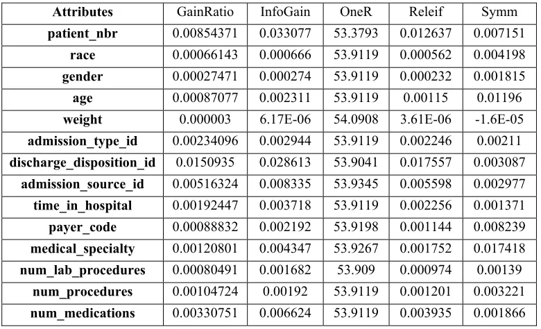
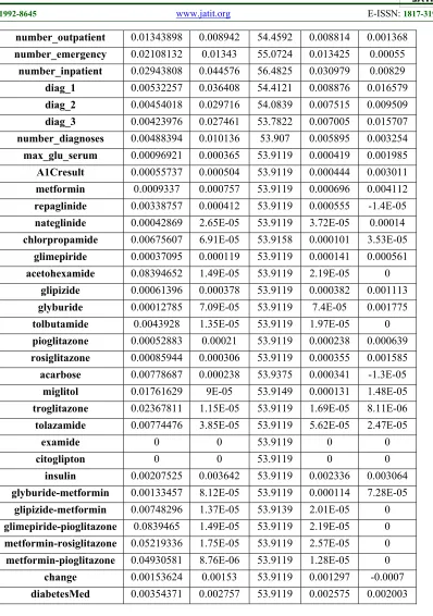
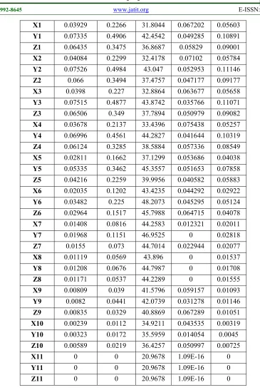
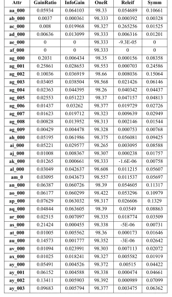
8383 and different class [32-35]. Symmetrical Uncertainty Attribute Evaluator: Evaluates the goodness of an attribute by measuring the symmetrical uncertainty for the class [36-37]. The result of applying those five mercies on five data sets is shown in Tables (1-5) in the appendix section respectively.

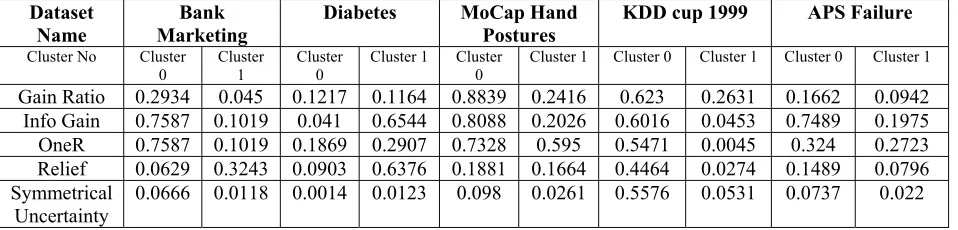
4.3Apply K-means Clustering on Datasets

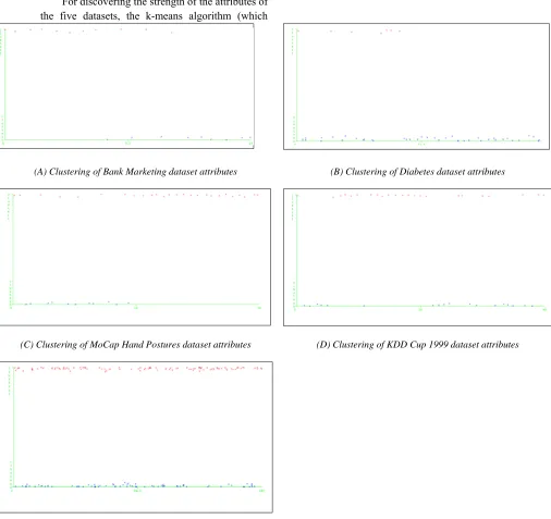
For discovering the strength of the attributes of the five datasets, the k-means algorithm (which

explained in Section 3.2) is applied to the data matrix that resulted from the previous step. For each dataset K-mean split the attributes between two clusters: weak and strong, the evaluation of cluster’s centroid of five datasets are shown in the Table 1 and Figure 2 present the clustering of attributes of the five datasets consecutively.

(A) Clustering of Bank Marketing dataset attributes (B) Clustering of Diabetes dataset attributes

(C) Clustering of MoCap Hand Postures dataset attributes (D) Clustering of KDD Cup 1999 dataset attributes

(E) Clustering of APS Failure dataset attributes

Figure 2: Clustering of attributes of five datasets

8384 Table 1: Evaluation of Cluster’s centroid of five datasets

4.4Apply Irrelevant Attributes Removal

Each attribute belongs to weak clusters from the previous step is removed resulting in a significant

reduction in the dimensionality of datasets. Table 2 clarifies the number of the attribute before and after applying the removal and the ration of attribute reduction.

Table 2: Ratio of Attributes Reduction in five datasets

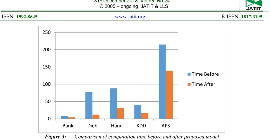
4.5Apply Bagging Classification

Bagging classification can be characterized by

creating the number of sub-dataset from the original dataset and applying classification processes in each one which represents a heavy computational time task. Thereby, the reduction of attributes number

provides the efficiency of bagging classification, especially with a big dataset. The improving of computational time on five datasets is shown in

Figure 3. Table 3 and Figures (4- 8) represent and illustrate the evaluation of bagging classification accuracy before and after applying the proposed model on five datasets.

Dataset Name Original Number of

attributes

Reduced Number of attributes Ratio of attributes Reduction

Bank Marketing 20 8 60%

Diabetes 48 41 15%

MoCap Hand

Postures 37 11 70%

KDD cup 1999 41 18 56%

APS Failure 170 71 58%

Dataset

Name Marketing Bank Diabetes MoCap Hand Postures KDD cup 1999 APS Failure

Cluster No Cluster

0 Cluster 1 Cluster 0 Cluster 1 Cluster 0 Cluster 1 Cluster 0 Cluster 1 Cluster 0 Cluster 1

Gain Ratio 0.2934 0.045 0.1217 0.1164 0.8839 0.2416 0.623 0.2631 0.1662 0.0942

Info Gain 0.7587 0.1019 0.041 0.6544 0.8088 0.2026 0.6016 0.0453 0.7489 0.1975

OneR 0.7587 0.1019 0.1869 0.2907 0.7328 0.595 0.5471 0.0045 0.324 0.2723

Relief 0.0629 0.3243 0.0903 0.6376 0.1881 0.1664 0.4464 0.0274 0.1489 0.0796

Symmetrical

8385

Figure 3: Comparison of computation time before and after proposed model

Table 3: Evaluation the accuracy before and after applying proposed model in five datasets

Figure 4: Comparison of bagging classification accuracy of Bank Marketing dataset before and after improvement 

Figure 5: Comparison of bagging classification accuracy of Diabetes dataset before and after improvement 

0 50 100 150 200 250

Bank Dieb Hand KDD APS

Time Before Time After

0 0.2 0.4 0.6 0.8 1

Before

After

0 0.2 0.4 0.6 0.8 1

Before

After

Dataset Name

Bank Marketing

Diabetes MoCap Hand Postures

KDD cup 1999 APS Failure

Before After Before After Before After Before After Before After TP Rate 0.912 0.905 0.533 0.534 0.942 0.891 0.999 0.999 0.966 0.967

Precision 0.894 0.871 0.478 0.482 0.942 0.891 0.999 0.999 0.965 0.967

Recall 0.912 0.905 0.533 0.534 0.942 0.891 0.999 0.999 0.966 0.967

F-Measure 0.894 0.871 0.492 0.497 0.942 0.891 0.999 0.999 0.965 0.967

8386 Figure6: Comparison of bagging classification accuracy of MoCap Hand Postures dataset before and after improvement

Figure7: Comparison of bagging classification accuracy of KDD cup 1999 dataset before and after improvement

Figure8: Comparison of bagging classification accuracy of APS Failure dataset before and after improvement

The performance of the classifier is measured by five common metrics as follow: (1) True Positive (TP), which related to the number of the positive examples that correctly predicted (2) Precision and (3) Recall which used widely in applications where the value of the successful detection of one of the classes is more significant than the detection of the other classes. Precision measures the fraction of the data rows that belong to the positive group, and the classifier has declared as a positive class. Recall calculates the fraction of positive examples that correctly predicted by the classifier [1].

Building a model that maximizes both precision and recall is the key challenge of the classification algorithms. Precision and recall can be summarized into another metric known as the (4) F1 measure as shown in equation (3).

F1 = 2* (Recall* Precision) / (Recall+ Precision) ………… (3)

(5) A receiver operating characteristic (ROC) curve is a graphical approach for displaying the tradeoff between true positive rate and false positive rate of a classifier. In a ROC curve, the true positive

rate (TPR) is plotted along the y-axis and the false positive rate (FPR) is shown on the x-axis [1, 2].

5.RESULTS DISCUSSIONS

To shed light on the proposed hybrid model results and their significant findings among other methods and approaches that have been proposed before to improve the classifications performance and its reliability, accuracy, effectiveness, and efficiency for high dimensional data. The proposed method is compared with some prior works regarding classification accuracy and consumed time. Table 4 shows that the proposed method has better classification accuracy and time for bank marketing dataset with 90.5 and 4.23 respectively.

Table 4: classification accuracy and time consumption for Bank marketing

work Classifier Accuracy Time (s)

2015 [38] MLPNN 88.63 1767.75

0.5 0.6 0.7 0.8 0.9 1

Before

After

0.5 0.6 0.7 0.8 0.9 1 1.1

Before

After

0.95 0.955 0.96 0.965 0.97 0.975 0.98 0.985 0.99 0.995

Before

8387

2016 [39]

LT-SVDD 90 4.96

Proposed

model Bagging 90.5 4.23

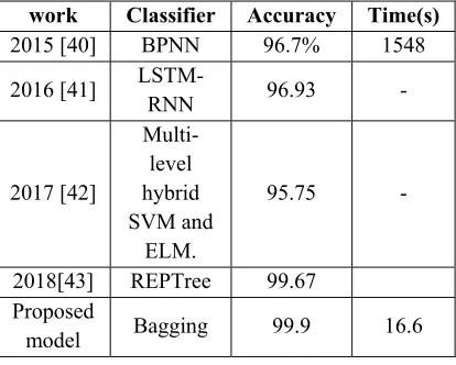
Table 5 shows that applying the proposed method on KDD Cup 1999 dataset is superior on five works regarding classification with accuracy 99.9 and it consumes 16.6 seconds compared with the work of Shah and Trivedi, who use back-propagation neural network algorithm for classification.

Table 5: classification accuracy and time consumption for KDD Cup 1999

work Classifier Accuracy Time(s)

2015 [40] BPNN 96.7% 1548

2016 [41]

LSTM-RNN 96.93 -

2017 [42] Multi-level hybrid SVM and ELM.

95.75 -

2018[43] REPTree 99.67

Proposed

model Bagging 99.9 16.6

Table 6 demonstrate that the proposed method has an accuracy better than the work of Schlag et al. for APS Failure dataset, but the consumption time is a little more.

Table 6: classification accuracy and time consumption for APS Failure

work Classifier Accuracy Time(s)

2018 [44] LPSVM 95 110.85

Proposed

model Bagging 96.7 139.36

6.CONCLUSIONS AND FUTURE WORK

In this article, a multi-phase model is proposed to eliminate irrelevant attributes with N number of goodness evaluation metrics via using K-Means Clustering and Bagging Ensemble Classifier. The hybrid model used the K-means clustering algorithm to discover the strength patterns of the attributes as well minimized data is classified using bagging ensemble techniques to improve the accuracy of the classification ( see Tables (1-5) in the appendix). The model is evaluated with five different datasets, and

the results were efficient due to its ability to deal with any number of metrics to reduce the attributes of the huge data up to (70%) (See Tables (4-6)). In the future directions, we intend to apply more advanced clustering techniques instead of k-means as well, applying soft computing techniques for choosing a suitable number of clusters.

REFERENCES:

[1] Han, Jiawei, Jian Pei, and Micheline Kamber. Data mining: concepts and techniques. Elsevier, 2011.

[2] Tan, Pang-Ning. Introduction to data mining. Pearson Education India, 2007.

[3] Amato, Giuseppe, et al. "How Data Mining and Machine Learning Evolved from Relational Data Base to Data Science." A Comprehensive Guide through the Italian Database Research over the Last 25 Years. Springer, Cham, 2018. 287-306.

[4] Gantz, John, and David Reinsel. "The digital universe in 2020: Big data, bigger digital shadows, and biggest growth in the far east." IDC iView: IDC Analyze the future 2007.2012 (2012): 1-16.

[5] Zhu, Pengfei, et al. "Unsupervised feature selection by regularized self-representation." Pattern Recognition 48.2 (2015): 438-446. [6] Witten, Ian H., et al. Data Mining: Practical

machine learning tools and techniques. Morgan Kaufmann, 2016.

[7] Sheikhpour, Razieh, et al. "A survey on semi-supervised feature selection methods." Pattern Recognition 64 (2017): 141-158.

[8] Chen, C.-H. (2015). Feature selection for clustering using instance-based learning by exploring the nearest and farthest neighbors. Information Sciences, 318, 14-27.

[9] Gondek, C., Hafner, D., & Sampson, O. R. (2016). Prediction of failures in the air pressure system of scania trucks using a random forest and feature engineering. Paper presented at the International Symposium on Intelligent Data Analysis.

[10] Hong, S.-S., Lee, W., & Han, M.-M. (2015). The feature selection method based on genetic algorithm for efficient of text clustering and text

classification. International Journal of

Advances in Soft Computing & Its Applications, 7(1).

8388 [12] Questier, F., Put, R., Coomans, D., Walczak, B.,

& Vander Heyden, Y. (2005). The use of CART and multivariate regression trees for supervised

and unsupervised feature selection.

Chemometrics and Intelligent Laboratory Systems, 76(1), 45-54.

[13] Ravale, U., Marathe, N., & Padiya, P. (2015). Feature selection based hybrid anomaly intrusion detection system using K means and RBF kernel function. Procedia Computer Science, 45, 428-435.

[14] Shang, R., Zhang, Z., Jiao, L., Liu, C., & Li, Y. (2016). Self-representation based dual-graph regularized feature selection clustering. Neurocomputing, 171, 1242-1253.

[15] Song, Q., Ni, J., & Wang, G. (2013). A fast clustering-based feature subset selection algorithm for high-dimensional data. IEEE Transactions on Knowledge and Data Engineering, 25(1), 1-14.

[16] Tabakhi, S., & Moradi, P. (2015). Relevance– redundancy feature selection based on ant colony optimization. Pattern recognition, 48(9), 2798-2811.

[17] Zhao, Z., He, X., Cai, D., Zhang, L., Ng, W., & Zhuang, Y. (2016). Graph regularized feature selection with data reconstruction. IEEE Transactions on Knowledge and Data Engineering, 28(3), 689-700.

[18] Zhu, P., Zuo, W., Zhang, L., Hu, Q., & Shiu, S. C. (2015). Unsupervised feature selection by

regularized self-representation. Pattern

recognition, 48(2), 438-446.

[19] Olson, David L. Descriptive data mining. Springer Singapore, 2017.

[20] Rokach, Lior, and Oded Z. Maimon. Data mining with decision trees: theory and applications. Vol. 69. World scientific, 2008. [21] Seni, Giovanni, and John F. Elder. "Ensemble

methods in data mining: improving accuracy through combining predictions." Synthesis Lectures on Data Mining and Knowledge Discovery 2.1 (2010): 1-126.

[22] Nisbet, Robert, John Elder, and Gary Miner. Handbook of statistical analysis and data mining applications. Academic Press, 2009.

[23] Altman, Naomi, and Martin Krzywinski. "Points of Significance: Ensemble methods: bagging and random forests." (2017): 933. [24] Catal, Cagatay, and Mehmet Nangir. "A

sentiment classification model based on multiple classifiers." Applied Soft Computing 50 (2017): 135-141.

[25] Moro, Sérgio, Paulo Cortez, and Paulo Rita. "A data-driven approach to predict the success of

bank telemarketing." Decision Support Systems 62 (2014): 22-31.

[26] Strack, Beata, et al. "Impact of HbA1c measurement on hospital readmission rates: analysis of 70,000 clinical database patient records." BioMed research international 2014 (2014).

[27] Gardner, Andrew, et al. "Measuring distance between unordered sets of different sizes." Proceedings of the IEEE Conference on Computer Vision and Pattern Recognition. 2014.

[28] Gardner, Andrew, et al. "3D hand posture recognition from small unlabeled point sets." Systems, Man and Cybernetics (SMC), 2014 IEEE International Conference on. IEEE, 2014. [29]

http://archive.ics.uci.edu/ml/machine-learning-databases/kddcup99-mld/

[30]https://archive.ics.uci.edu/ml/machine-learning-databases/00421/

[31] Holte, Robert C. "Very simple classification rules perform well on most commonly used datasets." Machine learning 11.1 (1993): 63-90. [32] Kira, Kenji, and Larry A. Rendell. "A practical approach to feature selection." Machine Learning Proceedings 1992. 1992. 249-256. [33] Katsifarakis, Nikos, and Kostas Karatzas. "A

New Feature Selection Methodology for Environmental Modelling Support: The Case of Thessaloniki Air Quality." Environmental Software Systems. Computer Science for Environmental Protection: 12th IFIP WG 5.11 International Symposium, ISESS 2017, Zadar, Croatia, May 10-12, 2017, Proceedings 12. Springer International Publishing, 2017.2603. [34] Kononenko, Igor. "Estimating attributes:

analysis and extensions of RELIEF." European conference on machine learning. Springer, Berlin, Heidelberg, 1994.

[35] Robnik-Šikonja, Marko, and Igor Kononenko. "An adaptation of Relief for attribute estimation in regression." Machine Learning: Proceedings of the Fourteenth International Conference (ICML’97). Vol. 5. 1997.

[36] Hall, Mark A., and Lloyd A. Smith. "Practical feature subset selection for machine learning." Computer science’98 proceedings of the 21st Australasian computer science conference ACSC. Vol. 98. 1998.

8389 [38] B. M. Shashidhara, et al., "Evaluation of

machine learning frameworks on bank marketing and Higgs datasets," in Advances in Computing and Communication Engineering

(ICACCE), 2015 Second International

Conference on, 2015, pp. 551-555.

[39] A. Rekha, et al., "Artificial Intelligence Marketing: An application of a novel Lightly Trained Support Vector Data Description," Journal of Information and Optimization Sciences, vol. 37, pp. 681-691, 2016.

[40] B. Shah and B. H. Trivedi, "Reducing features of KDD CUP 1999 dataset for anomaly detection using back propagation neural network," in Advanced Computing & Communication Technologies (ACCT), 2015 Fifth International Conference on, 2015, pp. 247-251.

[41] J. Kim, et al., "Long short term memory recurrent neural network classifier for intrusion detection," in Platform Technology and Service (PlatCon), 2016 International Conference on, 2016, pp. 1-5.

[42] W. L. Al-Yaseen, et al., "Multi-level hybrid support vector machine and extreme learning machine based on modified K-means for intrusion detection system," Expert Systems with Applications, vol. 67, pp. 296-303, 2017. [43] B. A. Tama and K.-H. Rhee, "An integration of

pso-based feature selection and random forest for anomaly detection in iot network," in MATEC Web of Conferences, 2018.

[44] S. Schlag, et al., "Faster Support Vector Machines," arXiv preprint arXiv:1808.06394, 2018.

8390

APPENDICES

Table 1: Bank Marketing Dataset Attributes Evaluation Using PART With Five Metrics

Attribute Name GainRatio InfoGain OneR Releif Symm

age 0.011883 0.018439 0.018439 0.0198 0.017905

job 0.004773 0.014223 0.014223 0.14063 0.008156

marital 0.001562 0.002069 0.002069 0.07408 0.002258

education 0.001349 0.003448 0.003448 0.14278 0.00225

default 0.011256 0.008331 0.008331 0.04785 0.01335

housing 8.78E-05 9.97E-05 9.97E-05 0.06619 0.000121

loan 0 1.93E-05 1.93E-05 0.04517 3.02E-05

contact 0.017742 0.016801 0.016801 0.01689 0.023097

month 0.014382 0.038097 0.038097 0.04081 0.024136

day_of_week 0.0002 0.000465 0.000465 0.20365 0.000328

duration 0.03364 0.109413 0.109413 0.06741 0.058192

campaign 0.002452 0.004285 0.004285 0.00336 0.003799

pdays 0.19567 0.044484 0.044484 0.0014 0.121009

previous 0.040006 0.027733 0.027733 0.0026 0.046179

poutcome 0.064022 0.043834 0.043834 0.01801 0.073514

emp.var.rate 0.034411 0.078586 0.078586 0.00433 0.056301

cons.price.idx 0.030057 0.098004 0.098004 0.00724 0.052012

cons.conf.idx 0.032945 0.097628 0.097628 0.00701 0.05625

euribor3m 0.030647 0.10257 0.10257 0.00373 0.053218

nr.employed 0.037894 0.08963 0.08963 0.00392 0.062391

Table 2: Diabetes Dataset Attributes Evaluation Using PART With Five Metrics

Attributes GainRatio InfoGain OneR Releif Symm

patient_nbr 0.00854371 0.033077 53.3793 0.012637 0.007151

race 0.00066143 0.000666 53.9119 0.000562 0.004198

gender 0.00027471 0.000274 53.9119 0.000232 0.001815

age 0.00087077 0.002311 53.9119 0.00115 0.01196

weight 0.000003 6.17E-06 54.0908 3.61E-06 -1.6E-05

admission_type_id 0.00234096 0.002944 53.9119 0.002246 0.00211

discharge_disposition_id 0.0150935 0.028613 53.9041 0.017557 0.003087

admission_source_id 0.00516324 0.008335 53.9345 0.005598 0.002977

time_in_hospital 0.00192447 0.003718 53.9119 0.002256 0.001371

payer_code 0.00088832 0.002192 53.9198 0.001144 0.008239

medical_specialty 0.00120801 0.004347 53.9267 0.001752 0.017418

num_lab_procedures 0.00080491 0.001682 53.909 0.000974 0.00139

num_procedures 0.00104724 0.00192 53.9119 0.001201 0.003221

8391

number_outpatient 0.01343898 0.008942 54.4592 0.008814 0.001368

number_emergency 0.02108132 0.01343 55.0724 0.013425 0.00055

number_inpatient 0.02943808 0.044576 56.4825 0.030979 0.00829

diag_1 0.00532257 0.036408 54.4121 0.008876 0.016579

diag_2 0.00454018 0.029716 54.0839 0.007515 0.009509

diag_3 0.00423976 0.027461 53.7822 0.007005 0.015707

number_diagnoses 0.00488394 0.010136 53.907 0.005895 0.003254

max_glu_serum 0.00096921 0.000365 53.9119 0.000419 0.001985

A1Cresult 0.00055737 0.000504 53.9119 0.000444 0.003011

metformin 0.0009337 0.000757 53.9119 0.000696 0.004112

repaglinide 0.00338757 0.000412 53.9119 0.000555 -1.4E-05

nateglinide 0.00042869 2.65E-05 53.9119 3.72E-05 0.00014

chlorpropamide 0.00675607 6.91E-05 53.9158 0.000101 3.53E-05

glimepiride 0.00037095 0.000119 53.9119 0.000141 0.000561

acetohexamide 0.08394652 1.49E-05 53.9119 2.19E-05 0

glipizide 0.00061396 0.000378 53.9119 0.000382 0.001113

glyburide 0.00012785 7.09E-05 53.9119 7.4E-05 0.001775

tolbutamide 0.0043928 1.35E-05 53.9119 1.97E-05 0

pioglitazone 0.00052883 0.00021 53.9119 0.000238 0.000639

rosiglitazone 0.00085944 0.000306 53.9119 0.000355 0.001585

acarbose 0.00778687 0.000238 53.9375 0.000341 -1.3E-05

miglitol 0.01761629 9E-05 53.9149 0.000131 1.48E-05

troglitazone 0.02367811 1.15E-05 53.9119 1.69E-05 8.11E-06

tolazamide 0.00774476 3.85E-05 53.9119 5.62E-05 2.47E-05

examide 0 0 53.9119 0 0

citoglipton 0 0 53.9119 0 0

insulin 0.00207525 0.003642 53.9119 0.002336 0.003064

glyburide-metformin 0.00133457 8.12E-05 53.9119 0.000114 7.28E-05

glipizide-metformin 0.00748296 1.37E-05 53.9139 2.01E-05 0

glimepiride-pioglitazone 0.0839465 1.49E-05 53.9119 2.19E-05 0

metformin-rosiglitazone 0.05219336 1.75E-05 53.9119 2.57E-05 0

metformin-pioglitazone 0.04930581 8.76E-06 53.9119 1.28E-05 0

change 0.00153624 0.00153 53.9119 0.001297 -0.0007

diabetesMed 0.00354371 0.002757 53.9119 0.002575 0.002003

Table 3: Mocap Hand Postures Dataset Attributes Evaluation Using PART With Five Metrics

Attr GainRatio InfoGain OneR Relief Symm User 0.00723 0.025 24.8259 0.269573 0.00865

X0 0.04299 0.2575 33.4089 0.068946 0.06197

Y0 0.07679 0.5093 43.1174 0.052394 0.11377

8392

X1 0.03929 0.2266 31.8044 0.067202 0.05603

Y1 0.07335 0.4906 42.4542 0.049285 0.10891

Z1 0.06435 0.3475 36.8687 0.05829 0.09001

X2 0.04084 0.2299 32.4178 0.07102 0.05784

Y2 0.07526 0.4984 43.047 0.052953 0.11146

Z2 0.066 0.3494 37.4757 0.047177 0.09177

X3 0.0398 0.227 32.8864 0.063677 0.05658

Y3 0.07515 0.4877 43.8742 0.035766 0.11071

Z3 0.06506 0.349 37.7894 0.050979 0.09082

X4 0.03678 0.2137 33.4396 0.075438 0.05257

Y4 0.06996 0.4561 44.2827 0.041644 0.10319

Z4 0.06124 0.3285 38.5884 0.057336 0.08549

X5 0.02811 0.1662 37.1299 0.053686 0.04038

Y5 0.05335 0.3462 45.3557 0.051653 0.07858

Z5 0.04216 0.2259 39.9956 0.040582 0.05883

X6 0.02035 0.1202 43.4235 0.044292 0.02922

Y6 0.03482 0.225 48.2073 0.045295 0.05124

Z6 0.02964 0.1517 45.7988 0.064715 0.04078

X7 0.01408 0.0816 44.2583 0.012321 0.02011

Y7 0.01968 0.1151 46.9525 0 0.02818

Z7 0.0155 0.073 44.7014 0.022944 0.02077

X8 0.01119 0.0569 43.896 0 0.01537

Y8 0.01208 0.0676 44.7987 0 0.01708

Z8 0.01171 0.0537 44.2289 0 0.01555

X9 0.00809 0.039 41.5796 0.059157 0.01093

Y9 0.0082 0.0441 42.0739 0.031278 0.01146

Z9 0.00835 0.0329 40.8869 0.067289 0.01051

X10 0.00239 0.0112 34.9211 0.043535 0.00319

Y10 0.00323 0.0172 35.5959 0.014054 0.0045

Z10 0.00589 0.0219 36.4257 0.050997 0.00725

X11 0 0 20.9678 1.09E-16 0

Y11 0 0 20.9678 1.09E-16 0

Z11 0 0 20.9678 1.09E-16 0

Table 4: KDD Cup 1999 Dataset Attributes Evaluation Using PART With Five Metrics

Attr GainRatio InfoGain OneR Releif Symm att1 0.128 0.02566 56.8012 0 0.02922

att2 0.7656 0.749869 78.0186 0.432155 0.591564

att3 0.6457 1.451671 98.5533 0.814374 0.763265

att4 0.8512 0.772744 76.7197 0.513637 0.627327

8393

att6 0.5103 0.787882 74.0475 0.000212 0.508336

att7 1 0.000327 56.8031 0.00027 0.00042

att8 1 0.002628 56.8164 0 0.003372

att9 0 0 56.8012 0 0

att10 0.4005 0.021701 56.9662 0.000645 0.026958

att11 0.3895 0.000696 56.8012 0 0.000894

att12 0.7146 0.714519 72.1516 0.502149 0.559174

att13 0.8068 0.018521 56.9747 2.82E-05 0.023463

att14 0 0 56.8012 2.86E-05 0

att15 0 0 56.8012 0 0

att16 0.0837 0.002199 56.8012 0 0.00278

att17 0.0782 0.001055 56.8012 4.77E-06 0.001344

att18 0 0 56.8012 1.91E-05 0

att19 0.084 0.002261 56.8012 0.001314 0.002857

att20 0 0 56.8012 0 0

att21 0 0 56.8012 0 0

att22 0.0818 0.001796 56.8012 0.001001 0.002276

att23 0.4221 1.377399 97.2753 0.365748 0.571693

att24 0.2411 0.870868 78.6338 0.301388 0.337019

att25 0.9196 0.747999 76.6139 0.500137 0.631441

att26 0.9121 0.715417 76.4165 0.499866 0.611424

att27 0.3496 0.07313 57.2818 0.026931 0.082869

att28 0.2555 0.057262 56.8012 0.025552 0.064344

att29 0.6087 0.744118 76.4813 0.403561 0.535693

att30 0.8348 0.752617 76.6015 0.045597 0.612545

att31 0.2221 0.245488 56.8012 0.086606 0.18451

att32 0.2735 0.457017 59.2769 0.29733 0.28327

att33 0.3934 0.752724 74.9154 0.396057 0.433954

att34 0.4369 0.761018 75.7308 0.322406 0.461578

att35 0.4044 0.741163 74.6645 0.069738 0.437476

att36 0.3965 0.910599 76.6739 0.393067 0.472727

att37 0.4206 0.431957 57.4783 0.023424 0.334491

att38 0.7876 0.752207 76.5223 0.480489 0.599183

att39 0.808 0.728052 76.4365 0.502253 0.592686

att40 0.2418 0.093149 57.1416 0.02713 0.095984

8394

Table 5: APS Failure At Scania Trucks Dataset Attributes Evaluation Using PART With Five Metrics

Attr GainRatio InfoGain OneR Releif Symm aa_000 0.05934 0.064103 98.33 0.054689 0.10661

ab_000 0.0037 0.000361 98.333 0.000392 0.00328

ac_000 0.008 0.019968 98.327 0.265256 0.01525

ad_000 0.00636 0.013099 98.333 0.006316 0.01201

ae_000 0 0 98.333 -9.3E-05 0

af_000 0 0 98.333 0 0

ag_000 0.2031 0.006434 98.35 0.000156 0.08358

ag_001 0.25861 0.028653 98.553 0.000703 0.24586

ag_002 0.10036 0.036919 98.66 0.008036 0.15064

ag_003 0.03405 0.038504 98.568 0.021426 0.06146

ag_004 0.02363 0.044395 98.26 0.040342 0.04437

ag_005 0.02553 0.051223 98.37 0.047157 0.04813

ag_006 0.01437 0.03262 98.377 0.019729 0.02726

ag_007 0.01623 0.019712 98.323 0.009639 0.02949

ag_008 0.00828 0.013952 98.313 0.002146 0.01544

ag_009 0.00429 0.004478 98.328 0.000753 0.00768

ah_000 0.05195 0.061986 98.375 0.056081 0.09425

ai_000 0.05221 0.029577 98.265 0.003095 0.08588

aj_000 0.01008 0.008367 98.307 0.000238 0.01757

ak_000 0.01265 0.000661 98.333 -1.6E-06 0.00758

al_000 0.03049 0.042637 98.608 0.011215 0.05607

am_0 0.03095 0.043673 98.557 0.011537 0.05697

an_000 0.06387 0.060726 98.39 0.054605 0.11317

ao_000 0.06177 0.060299 98.422 0.053296 0.10979

ap_000 0.07629 0.063032 98.317 0.026606 0.1329

aq_000 0.04844 0.063605 98.39 0.03549 0.08863

ar_000 0.02515 0.007097 98.335 0.018774 0.03509

as_000 0.21424 0.000455 98.338 -5E-06 0.00731

at_000 0.01005 0.005562 98.36 0.000173 0.01646

au_000 0.14573 0.001777 98.352 -3E-06 0.02642

av_000 0.01094 0.023991 98.303 0.007113 0.02072

ax_000 0.01025 0.018241 98.327 0.005582 0.01919

ay_000 0.05491 0.004526 98.372 0.00515 0.04422

ay_001 0.06152 0.004588 98.338 0.000474 0.04661

ay_002 0.13411 0.005903 98.392 0.000989 0.07099

8395

ay_004 0.03603 0.008809 98.405 0.001471 0.04804

ay_005 0.01276 0.016536 98.367 0.001761 0.02331

ay_006 0.01228 0.0177 98.332 0.01994 0.02263

ay_007 0.01706 0.034644 98.205 0.012751 0.03218

ay_008 0.04585 0.037672 98.3 0.039881 0.07982

ay_009 0.16956 0.013839 98.452 0.027207 0.13574

az_000 0.0347 0.052378 98.263 0.005495 0.06419

az_001 0.03004 0.050065 98.397 0.008983 0.05597

az_002 0.02984 0.050026 98.413 0.001489 0.05563

az_003 0.01022 0.019601 98.305 0.00305 0.01921

az_004 0.01439 0.03291 98.308 0.0141 0.02732

az_005 0.0275 0.04772 98.298 0.039267 0.05137

az_006 0.00526 0.008302 98.327 0.009957 0.00977

az_007 0.01168 0.016143 98.403 0.034495 0.02146

az_008 0.01312 0.007291 98.333 8.3E-05 0.02151

az_009 0.0203 0.004705 98.33 -9.5E-05 0.02658

ba_000 0.03624 0.051533 98.343 0.033332 0.06674

ba_001 0.0278 0.050886 98.283 0.027294 0.05212

ba_002 0.0437 0.051837 98.212 0.039741 0.07923

ba_003 0.02831 0.052333 98.38 0.031388 0.05311

ba_004 0.02873 0.051322 98.398 0.027023 0.05378

ba_005 0.02339 0.046223 98.38 0.027373 0.04405

ba_006 0.02024 0.038741 98.267 0.019439 0.03805

ba_007 0.01437 0.030778 98.287 0.025147 0.02718

ba_008 0.02335 0.029829 98.278 0.016011 0.04263

ba_009 0.02497 0.024091 98.298 0.029467 0.04433

bb_000 0.05867 0.063643 98.397 0.043317 0.10545

bc_000 0.00954 0.019603 98.297 0.016249 0.01801

bd_000 0.01116 0.027465 98.307 0.00295 0.02127

be_000 0.01158 0.023246 98.327 0.006178 0.02183

bf_000 0.00659 0.008907 98.325 0.00696 0.01209

bg_000 0.05181 0.061828 98.372 0.056242 0.09399

bh_000 0.06955 0.06131 98.308 0.031641 0.12216

bi_000 0.03628 0.055474 98.273 0.012981 0.06718

bj_000 0.06444 0.065734 98.372 0.026949 0.11509

bk_000 0.0159 0.026885 98.377 0.121054 0.02965

bl_000 0.01282 0.024102 98.31 0.132517 0.02408

bm_000 0.01971 0.032717 98.292 0.135327 0.03671

bn_000 0.02835 0.038516 98.332 0.136182 0.05201

bo_000 0.0365 0.041953 98.218 0.124863 0.06599

8396

bq_000 0.04879 0.047191 98.265 0.123496 0.08663

br_000 0.05614 0.048837 98.275 0.135879 0.09845

bs_000 0.00805 0.016204 98.315 0.07371 0.01518

bt_000 0.04907 0.063862 98.313 0.044541 0.0897

bu_000 0.05842 0.063498 98.385 0.043334 0.10503

bv_000 0.05842 0.063498 98.387 0.043334 0.10503

bx_000 0.03845 0.056801 98.345 0.04071 0.07103

by_000 0.0282 0.054189 98.383 0.04887 0.05303

bz_000 0.00445 0.009077 98.322 0.003295 0.0084

ca_000 0.01565 0.020494 98.333 0.241526 0.02863

cb_000 0.00336 0.005144 98.333 0.22544 0.00622

cc_000 0.04115 0.057691 98.382 0.048707 0.0757

cd_000 0.00733 0.000653 98.333 0.122922 0.00618

ce_000 0.0215 0.029061 98.313 0.064487 0.03943

cf_000 0.01004 0.011734 98.322 -6.8E-05 0.01818

cg_000 0.00994 0.018784 98.333 0.010246 0.01867

ch_000 0 0 98.333 0 0

ci_000 0.06587 0.065802 98.365 0.050465 0.11737

cj_000 0.02007 0.019744 98.428 0.011239 0.0357

ck_000 0.05382 0.064663 98.24 0.041375 0.09769

cl_000 0.05676 0.021218 98.293 0.002331 0.08553

cm_000 0.0118 0.022537 98.342 0.019454 0.02217

cn_000 0.11947 0.030809 98.573 0.00315 0.16208

cn_001 0.04297 0.034653 98.585 0.01532 0.07462

cn_002 0.02362 0.036825 98.352 0.022375 0.04381

cn_003 0.03459 0.048335 98.258 0.03386 0.06362

cn_004 0.03719 0.05018 98.365 0.032132 0.0682

cn_005 0.01849 0.03696 98.292 0.021867 0.03485

cn_006 0.01171 0.026223 98.257 0.012264 0.02221

cn_007 0.0117 0.027664 98.242 0.017329 0.02225

cn_008 0.01791 0.02684 98.308 0.021227 0.03312

cn_009 0.00919 0.017001 98.322 0.011429 0.01724

co_000 0.00318 0.006098 98.337 0.00423 0.00597

cp_000 0.00931 0.017557 98.332 0.00209 0.01749

cq_000 0.05842 0.063498 98.385 0.043334 0.10503

cr_000 0.0542 0.000405 98.333 1.1E-06 0.00624

cs_000 0.02061 0.040013 98.275 0.036672 0.03877

cs_001 0.02382 0.044337 98.293 0.035575 0.04471

cs_002 0.0431 0.05406 98.207 0.031969 0.07855

cs_003 0.02856 0.049523 98.222 0.016504 0.05336

8397

cs_005 0.02573 0.047213 98.322 0.036052 0.04825

cs_006 0.02329 0.020401 98.287 0.031197 0.04087

cs_007 0.00719 0.017691 98.33 0.00127 0.01369

cs_008 0.00312 0.006113 98.332 7.06E-05 0.00587

cs_009 0.03865 0.00024 98.333 -1E-05 0.00373

ct_000 0.00575 0.012877 98.328 0.01099 0.0109

cu_000 0.00806 0.016207 98.315 0.00176 0.01519

cv_000 0.01335 0.026995 98.283 0.063609 0.02518

cx_000 0.01283 0.025099 98.302 0.033665 0.02415

cy_000 0.02075 0.003221 98.328 0.002444 0.02321

cz_000 0.00304 0.005964 98.327 0.001869 0.00573

da_000 0 0 98.333 -8.3E-05 0

db_000 0.00829 0.007537 98.333 0 0.01462

dc_000 0.01395 0.027909 98.298 0.041415 0.02629

dd_000 0.02812 0.045678 98.248 0.023877 0.05231

de_000 0.02132 0.033453 98.315 0.00985 0.03956

df_000 0.20795 0.003311 98.338 0.003541 0.04791

dg_000 0.02796 0.004606 98.378 0.003945 0.03209

dh_000 0.00319 0.002165 98.333 -1.6E-05 0.00541

di_000 0.00792 0.006573 98.34 0.002364 0.01381

dj_000 0 0 98.333 -2.8E-06 0

dk_000 0 0 98.333 -7.5E-05 0

dl_000 0 0 98.333 3.88E-05 0

dm_000 0 0 98.333 1.73E-05 0

dn_000 0.05118 0.063722 98.355 0.036472 0.0932

do_000 0.01097 0.020683 98.357 0.035351 0.0206

dp_000 0.00756 0.020634 98.36 0.02892 0.01446

dq_000 0.0083 0.00836 98.315 0.011692 0.0148

dr_000 0.00817 0.009199 98.297 0.023004 0.01474

ds_000 0.0212 0.041745 98.277 0.051881 0.03991

dt_000 0.02198 0.041382 98.358 0.062894 0.04128

du_000 0.01184 0.01926 98.317 0.01844 0.02202

dv_000 0.01316 0.021831 98.305 0.005467 0.02451

dx_000 0.00672 0.008785 98.31 0.034744 0.01229

dy_000 0.00596 0.008663 98.323 0.003061 0.01099

dz_000 0.03985 0.000165 98.33 -1.9E-06 0.00261

ea_000 0.00342 0.000359 98.333 -5.8E-05 0.00316

eb_000 0.00684 0.013875 98.337 0.011118 0.0129

ec_00 0.01851 0.032031 98.338 0.018058 0.03458

ed_000 0.01843 0.034386 98.27 0.023878 0.03459

8398

ee_001 0.0219 0.04754 98.293 0.014519 0.04146

ee_002 0.0234 0.048593 98.397 0.039534 0.0442

ee_003 0.0219 0.045201 98.367 0.021799 0.04134

ee_004 0.0232 0.043646 98.328 0.02856 0.04357

ee_005 0.03075 0.048769 98.573 0.039454 0.0571

ee_006 0.01687 0.039952 98.385 0.026574 0.03209

ee_007 0.02463 0.024192 98.277 0.018198 0.04381

ee_008 0.009 0.016591 98.335 0.005648 0.01688

ee_009 0.00322 0.005551 98.323 0 0.00602

ef_000 0.02384 0.000195 98.332 1.44E-05 0.00299