Functionals of exponential Brownian motion and divided differences

BIROn - Birkbeck Institutional Research Online

Baxter, Brad J.C. and Brummelhuis, Raymond (2011) Functionals of

exponential Brownian motion and divided differences.

Journal of

Computational and Applied Mathematics 236 (4), pp. 424-433. ISSN

0377-0427.

Downloaded from:

Usage Guidelines:

Please refer to usage guidelines at

or alternatively

BIROn -

B

irkbeck

I

nstitutional

R

esearch

On

line

Enabling open access to Birkbeck’s published research output

Functionals of exponential Brownian motion and divided

differences

Journal Article

http://eprints.bbk.ac.uk/3050

Version: Post-print (refereed)

Citation:

© 2011 – Wiley Blackwell

Publisher version vailable upon publication

______________________________________________________________

All articles available through Birkbeck ePrints are protected by intellectual property law, including copyright law. Any use made of the contents should comply with the relevant law.

______________________________________________________________

Deposit Guide

Contact: [email protected]

Birkbeck ePrints

Birkbeck ePrints

Baxter, B.; Brummelhuis, B. (2011) Functionals of exponential

Brownian motion and divided differences –

FUNCTIONALS OF EXPONENTIAL BROWNIAN MOTION AND DIVIDED DIFFERENCES

B. J. C. BAXTER AND R. BRUMMELHUIS

Abstract. We provide a surprising new application of classical approximation theory to a fundamental asset-pricing model of mathematical finance. Specif-ically, we calculate an analytic value for the correlation coefficient between exponential Brownian motion and its time average, and we find the use of di-vided differences greatly elucidates formulae, providing a path to several new results. As applications, we find that this correlation coefficient is always at least 1/√

2 and, via the Hermite–Genocchi integral relation, demonstrate that all moments of the time average are certain divided differences of the expo-nential function. We also prove that these moments agree with the somewhat more complex formulae obtained by Oshanin and Yor.

1. Introduction

We begin with exponential, or geometric, Brownian motion, defined by

(1.1) S(t) =e(r−σ

2

2 )t+σB(t), t≥0,

whererandσare non-negative constants, andB: [0,∞)→R_{is Brownian motion.} In other words,B is a stochastic process, orrandom function, for whichB(0) = 1, its increments are independent, and, for 0 ≤s < t, the incrementB(t)−B(s) is normally distributed with mean zero and variance t−s. The basic properties of Brownian motion are explained in Section 37 of Billingsley (1995), while Karatzas and Shreve (1991) is a comprehensive treatise.

We shall study thetime average

(1.2) A(T) := 1

T

Z T

0

S(t)dt

using the calculus of divided differences, a fundamental tool in approximation the-ory. We will, in particular, show that the correlation coefficient betweenA(T) and

S(T), the moments ofA(T) and, more generally, joint moments ofS(T) andA(T) can be elegantly, and usefully, expressed in terms of divided differences of the ex-ponential function. Now the time averageA(T) has been extensively studied in the literature of Asian options; see, for instance, Yor (2001) and Oshanin, Mogutov and Moreau (1993). However, we find that our use of divided differences both simplify and elucidate formulae. In Section 2, we derive the correlation coefficient forS(T) andA(T), finding that it is always at least 1/√2, thus explaining the relative high correlation that is observational folklore in the financial community. In Section 3, we demonstrate that the divided differences occurring in the lower moments of

S(T) and A(T) generalise to all moments, using the fact that the integral of an exponential function over a simplex can be expressed, via the Hermite–Gennocchi formula, as a certain divided difference of the exponential function. In Section 4, we provide the divided difference theory required by the paper. Finally, in Section 5, we use our divided difference approach to derive a recurrence relation for the moments ofA(T).

Key words and phrases. Brownian motion, moments, divided differences, Asian options.

We first observe the familiar result

(1.3) E_{S(T) =e}(r−σ2/2)TE_eσT1/2Z_=e(r−σ2/2)T_eσ2T /2_=erT_.

Here Z denotes a generic N(0,1) Gaussian random variable and we have used the standard fact that

(1.4) E_eλZ _{= (2π)}−1/2

Z

R

eλτe−τ2/2dτ = (2π)−1/2

Z

R

e−12{(τ−λ) 2

−λ2

}_{dτ =e}λ2 /2_.

Similarly,

E_{A(T) = T}−1

Z T

0

E_S(t)dt

= e

rT ₋₁

rT .

(1.5)

The approximation theorist will immediately recognise the divided difference (1.6) E_{A(T) = exp[0, rT],}

but a sceptical reader might view this as mere coincidence; in fact, it is but the tip of an iceberg. We remind the reader that f[a0, a1, . . . , an] is the highest coefficient of

the unique polynomial of degreeninterpolatingf at distinct pointsa0, . . . , an∈R,

which implies f[a0] =f(a0) and

f[a0, a1] =

f(a1)−f(a0)

a1−a0

.

Further, it is evident that a divided difference does not depend on the order in which the pointsa0, a1, . . . , an are chosen. As mentioned above, Section 4 collects

further divided difference theory required by this paper.

2. The correlation coefficient between the time average and the asset

We shall compute the correlation coefficient between S(T) and A(T). Specifi-cally, we calculate

(2.1) R:= E(S(T)pA(T))−E(S(T))E(A(T))

varS(T) varA(T) . We find an elegant divided difference expression forR.

Theorem 2.1. The correlation coefficient (2.1)is given by

(2.2) R≡R(rT, σ2T) = exp[rT,2rT,(2r+σ

2_)T]

p

2 exp[2rT,(2r+σ2_{)T] exp[0, rT,2rT,(2r+σ}2_)T].

Let us begin our derivation.

Lemma 2.2. If0≤a≤b, then

(2.3) E_{S(a)S(b) = expa(r+σ}2_{) +br.}

Proof. We have

E_{S(a)S(b) =} E_S(a)2_e(b−a)(r−σ2/2)+σ(B(b)−B(a)) = E_S(a)2E_e(b−a)(r−σ2/2)+σ√b−aZ = e(2r+σ2

)a_e(b−a)r

= ea(r+σ2))ebr,

(2.4)

FUNCTIONALS OF EXPONENTIAL BROWNIAN MOTION AND DIVIDED DIFFERENCES 3

Proposition 2.3. We have

(2.5) E_{S(T)A(T) = exp[rT,(2r+σ}2_)T].

Proof. Applying Lemma 2.2, we obtain

E_{S(T)A(T) = T}−1

Z T

0

E_S(t)S(T)dt

= T−1

Z T

0

e(r+σ2)terTdt

= exp[rT,(2r+σ2)T].

Proposition 2.4.

(2.6) E_(A(T)2_{) = 2 exp[0, rT,(2r+σ}2_)T].

Proof. We find

E_(A(T)2_{) = T}−2

Z T

0

Z T

0

E_{S(t1)S(t2)dt2dt1}

= 2T−2

Z T

0

Z t1

0

E_{S(t1)S(t2)dt2dt1.} (2.7)

Thus

E_(A(T)2_{) = 2T}−2

Z T

0

Z t1

0

er(t1+t2)

eσ2t2

dt2

dt1

= 2T−2

Z T

0

ert1

e(r+σ

2

)t1

−1

r+σ2

dt1

= 2

(r+σ2_)T

exp[0,(2r+σ2_{)T]−exp[0, rT]}

= 2 exp[0, rT,(2r+σ2_)T],

(2.8)

using the divided difference recurrence relation (4.1) to obtain the final line.

Any reader still doubtful of the simplification provided by divided difference nota-tion might consider the alternative expression provided in Hull (2000):

E _A(T)2

= 2e

(2r+σ2

)T

(r+σ2_)(2r+σ2_)T2 +

2

rT2

1 2r+σ2 −

erT

r+σ2

.

There is a similar divided difference relation for E_(A(T)m_{), described in the next} section, but we now complete our derivation of Theorem 2.1.

Proof of Theorem 2.1. Applying (1.4, 1.5, 2.5) and (4.1), we obtain

E_S(T)A(T)−E_S(T)E_{A(T) = exp[rT,(2r+σ}2_)T]−erT_(erT _−1)/(rT) = exp[rT,(2r+σ2)T]−exp[rT,2rT] = σ2Texp[rT,2rT,(2r+σ2)T].

(2.9)

Further, (2.10)

and, by (1.5, 2.6),

varA(T) = 2 exp[0, rT,(2r+σ2)T]−

erT ₋₁

rT

2

= 2 exp[0, rT,(2r+σ2)T]−2 exp[0, rT,2rT] = 2σ2_{Texp[0, rT,2rT,(2r+σ}2_)T],

(2.11)

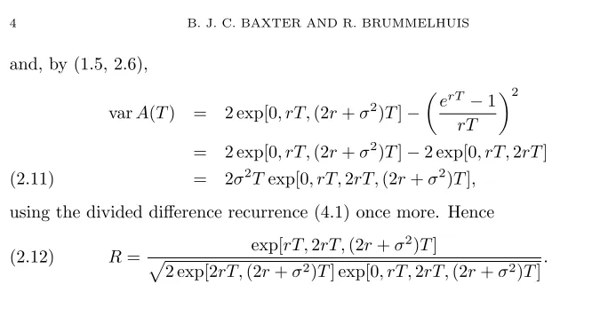
using the divided difference recurrence (4.1) once more. Hence

(2.12) R= exp[rT,2rT,(2r+σ

2_)T]

p

2 exp[2rT,(2r+σ2_{)T] exp[0, rT,2rT,(2r+σ}2_)T].

It is remarkable that the divided differences appearing in (2.12) are coefficients of the cubic polynomial interpolating the exponential function at 0, rT,2rT,(2r+σ2_)T.

We make three further observations:

(1) Armed with an analytic expression for the correlation coefficient, we can apply the exchange option valuation formula of Margrabe (1978) to derive the values of certain Asian options, if we are willing to accept that the time–average is suitably approximated by exponential Brownian motion. We are investigating the numerics of this rather simple approximation at present and preliminary results are surprisingly promising.

(2) The correlation coefficient R(rT, σ2_{T) is typically close to unity: typical}

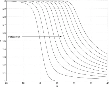
values ofr,σandTproduce values ofRin the 0.8−0.9 range. In fact, we are able to prove that the correlation coefficient satisfies R(rT, σ2_T)≥1/√_2,

for all r ≥ 0, σ ≥ 0 and T > 0, a surprisingly high lower bound for the correlation coefficient. The details of this derivation are too complicated to include here, and we refer the reader to Baxter and Fretwell (2011) for further details. However, the numerical findings are summarised in Figure 1, which displays values of the closely related quantity

S≡S(r, a) = (exp[a,2r, r])

2

exp[a,2r] exp[a,2r, r,0],

for−20≤a≤40 and 0.1≤r≤10. It is easily checked thatR(rT, σ2_{T) =}

p

S(rT,(2r+σ2_{)T)/2, so that the lower boundR≥1/}√_{2 becomesS≥1.}

It is plausible that S(r, a) should be a decreasing function ofa, for fixedr, because correlation should be a decreasing function of volatility. Further, it is not difficult to establish the limiting values lima→−∞S(a, r) = 2 and

limr→∞S(a, r) = 1. However, further analysis is not straightforward, and

the analysis of Baxter and Fretwell (2011) makes great use of properties of divided differences.

(3) It is natural to ask whether these divided difference expressions are particu-lar to exponential Brownian motion. In fact, simiparticu-lar expressions occur when exponential Brownian motion is replaced by certain L´evy-stable variants: see Baxter and Fretwell (2011) for further details.

3. Computing higher moments of A(T)

FUNCTIONALS OF EXPONENTIAL BROWNIAN MOTION AND DIVIDED DIFFERENCES 5

−201 −10 0 10 20 30 40

1.1 1.2 1.3 1.4 1.5 1.6 1.7 1.8 1.9 2

a

S

Increasing r

Figure 1. S(r, a) for−20≤a≤40 and 0.1≤r≤10

We begin with the iterated integral

(3.1) E_A(T)m_=T−m

Z T

0

dτm

Z T

0

dτm−1· · ·

Z T

0

dτ1 ES(τ1)· · ·S(τm).

Now, given any point (τ1, . . . , τm)∈[0, T]m, let us sort its components into

increas-ing order, obtainincreas-ing (t1, . . . , tn) (say). Then

E_{S(τ1)· · ·S(τm) =}E_{S(t1)· · ·S(tm)} and

(3.2) E_A(T)m_=m!T−m

Z T

0

dtm

Z tm

0

dtm−1· · ·

Z t2

0

dt1ES(t1)· · ·S(tm).

Our first task is to calculate the integrand, which we complete after a simple lemma.

Lemma 3.1. For any positive integerk, we have

(3.3) E

S(t)k

= expkrt+σ

2_t

2 k(k−1)

.

Proof. This is almost immediate from (1.4):

E_S(t)k ₌E_ek(r−σ2)t+σk√tZ_=ek(r−σ2/2)t+σ2k2t/2_=ekrt+σ2tk(k−1)/2_,

Proposition 3.2. If0≤t1≤t2≤ · · · ≤tm, then

(3.4) E_{S(t1)S(t2)· · ·S(tm) = exp}

m

X

k=1

r+ (m−k)σ2

tk

.

Proof. Lemma 2.2 comprises the case m= 2. We complete the proof by induction on the number of termsm, first observing that, by a standard property of geometric Brownian motion,

(3.5) E_{S(t1)S(t2)· · ·S(tm) =}E_S(t1)mE_{S(t2−t1)· · ·S(tm−t1).} Applying Lemma 3.1 and our induction hypothesis, we obtain

(3.6)

E_{S(t1)S(t2)· · ·S(tm) = expmrt1+σ}2_{t1m(m−1)/2+}

m

X

ℓ=2

r+ (m−ℓ)σ2

(tℓ−t1)

.

Thet1coefficient in the exponent is given by

mr−(m−1)r+σ2t1

1

2m(m−1)−

m−2

X

ℓ=1

ℓ

!

=r+σ2t1(m−1),

using the elementary fact thatm(m−1)/2 = 1 + 2 +· · ·+m−1. The coefficients oft2, . . . , tm are as already stated in (3.4).

Thus the desired integral (3.2) becomes

E_A(T)m _{= m!T}−m

Z T

0

dtm

Z tm

0

dtm−1· · ·

Z t2

0

dt1ES(t1)· · ·S(tm)

= m!

Z 1

0

dtm

Z tm−1

0 · · ·

Z t2

0

dt1exp(α1t1+· · ·αmtm),

(3.7)

where

(3.8) αk= r+ (m−k)σ2T, k= 1, . . . , m.

The integral displayed in (3.7) can now be identified as a divided difference using a variant form of the Hermite–Genocchi integral relation.

Theorem 3.3. Let

(3.9) bk:=kr+σ2k(k−1)/2, k= 0,1, . . . .

Then

(3.10) E_(A(T))m_{=m! exp[b0T, b1T, . . . , bmT], m≥0.}

Proof. Apply Corollary 4.5 to (3.7) and (3.8), usingPj

k=1k=j(j+ 1)/2.

The statement of Theorem 3.3 simplifies when r =σ2_{, for then the drift term}

in (1.1) vanishes, that is, we consider S(t) = exp(σ√tB(t)) alone; this is the spe-cial case studied by Oshanin et al. (1993) and Yor (2001), for the formulae grow

much more complicated without the use of divided differences. Therefore we now demonstrate that our expression agrees with theirs.

Theorem 3.4. If we setr=σ2_{/2 in Theorem 3.3, then we obtain}

E_[A(T)m_{] =m! exp[0, rT,2}2_rT,32_{rT, . . . , m}2_rT] =m!H√

rT[−m, . . . ,−1,0,1, . . . , m],

(3.11)

FUNCTIONALS OF EXPONENTIAL BROWNIAN MOTION AND DIVIDED DIFFERENCES 7

Proof. We simply setr=σ2 in Theorem 3.3 and apply (4.12).

We can now apply Corollary 4.10 to derive the formula given in equation (14) of Oshanin et al. (1993).

Theorem 3.5. If we setr=σ2_{/2, then}

(3.12)

E_[A(T)m_{] =}

Γ(m) Γ(2m)

r−m −1₂(−1)m

2m m + m X ℓ=0 2m ℓ

(−1)ℓerT(m−ℓ)2

!

.

Proof. Applying Corollary 4.10 to Theorem 3.4, we obtain

E_[A(T)m_{] =} m! (2m)!(rT)

−m 2m X k=0 _2m k

(−1)kerT(k−m)2

!

=

Γ(m) Γ(2m)

(rT)−m −1₂(−1)m

2m m + m X ℓ=0 2m ℓ

(−1)ℓerT(m−ℓ)2

!

,

(3.13)

after some straightforward algebraic manipulation.

If we now replace rT by αandm byj in (3.12), then we obtain equation (14) of Oshanin et al. (1993).

4. Divided difference theory

Most of the properties of divided differences required here can be found in Chap-ter 5 of Powell (1981) or ChapChap-ter 1 of de Boor (1978). There is also much useful material in Chapter 7 of the treatise of DeVore and Lorentz (1993), or indeed the original Hermite (1878).

We recall the divided difference recurrence relation.

Theorem 4.1.

(4.1) f[a0, a1, . . . , an] =

f[a1, . . . , an]−f[a0, . . . , an−1]

an−a0 ,

for any distinct complex numbersa0, . . . , an.

Proof. See, for instance, Powell (1981), Theorem 5.3.

Iff is sufficiently differentiable, then we can, of course, define divided differences for coincident points. Further, the elementary relation

(4.2) f[a0, a1] =

f(a1)−f(a0)

a1−a0

=

Z 1

0

f′((1−t)a0+ta1)dt, whena0, a1∈R,

can be generalised to obtain theHermite–Genocchi formula.

Theorem 4.2(Hermite–Genocchi). Let f ∈C(n)_{(R)and leta}

0, a1, . . . , an be (not

necessarily distinct) real numbers Then, for n≥1,

f[a0, a1, . . . , an]

=

Z

Sn

f(n)(t0a0+t1a1+· · ·+tnan)dt1· · ·dtn,

=

Z 1

0

dt1

Z 1−t1

0

dt2· · ·

Z 1−Pn−

1

k=1tk

0

dtnf(n)(t0a0+t1a1+· · ·+tnan)

(4.3)

where the domain of integration is the simplex

(4.4) Sn =

(

t= (t1, t2, . . . , tn)∈Rn+:

n

X

k=1

tk≤1

and

t0= 1−

n

X

k=1

tk.

Proof. A laconic derivation is given in Chapter 4, Section 7(k) of DeVore and

Lorentz (1993).

We shall need a variant form of the Hermite–Genocchi integral relation for which the following notation is useful. Given any real n×nnonsingular matrixV, with columns v1, . . . , vn, we letK(V) denote the closed convex hull of 0, v1, . . . , vn, i.e.

K(V) := conv{0, v1, . . . , vn}.

In this notation, the Hermite–Gnocchi integral relation states that

(4.5) f[a0, a1, . . . , an] =

Z

K(In)

f(n)a0+ (a−a0e)Ty

dy, where a=    a1 .. . an  

, e=

   1 .. . 1   ,

and In denotes the n×n identity matrix. Integrating thenth derivative over the

simplex K(V) yields a useful variant form of Hermite–Genocchi.

Theorem 4.3. LetV ∈Rn×n _{be any nonsingular matrix. Then}

(4.6) 1

|detV| Z

K(V)

f(n) aTy

dy=f[0,(VTa)1, . . . ,(VTa)n],

where (VTa)k denotes the kth component of the vectorVTa.

Proof. Substitutingy=V z, Hermite–Genocchi implies the relation

Z

K(V)

f(n) (VTa)Tz

dz=f[0,(VTa)1, . . . ,(VTa)n].

Corollary 4.4. For any function f ∈C(n)_{(R), we have}

Z 1

0

dxn

Z xn

0

dxn−1· · ·

Z x2

0

dx1f(n)

n

X

k=1

akxk

!

=f[0, an, an+an−1, . . . , an+an−1+· · ·+a1].

(4.7) Proof. Set V =      1 1 1 .. . . ..

1 1 · · · 1



   

in Theorem 4.3.

The exponential function is a particularly important case for us, in which case the Hermite–Genocchi formula becomes

(4.8) exp[a0, a1, . . . , an] =

Z

Sn

et0a0+t1a1+···+tnan_dt

1· · ·dtn

FUNCTIONALS OF EXPONENTIAL BROWNIAN MOTION AND DIVIDED DIFFERENCES 9

Corollary 4.5. We have

Z 1

0

dxn

Z xn

0

dxn−1· · ·

Z x2

0

dx1exp

n

X

k=1

akxk

!

= exp[0, an, an+an−1, . . . , an+an−1+· · ·+a1].

(4.9)

Proof. Letf be the exponential function in Corollary 4.4.

Further, we note that, for the exponential function, Theorem 4.3 becomes the interesting formula

(4.10) 1

|detV| Z

K(V)

eaTydy= exp[0,(VTa)1, . . . ,(VTa)n].

Thus, integrating exponentials over simplexes or, more generally, a polyhedron formed by the disjoint union of simplexes, will generate divided differences of the exponential.

We shall also need two simple preliminary results. Let us use P_{n to denote the} vector space of polynomials of degree n.

Lemma 4.6. We have

(4.11) exp(µ) exp[λ0, . . . , λm] = exp[λ0+µ, . . . , λm+µ],

where λ0, . . . , λm andµcan be any complex numbers.

Proof. Immediate.

Lemma 4.7. Letf:C_→C_{and leta1, . . . , anbe distinct nonzero complex numbers.}

Then

(4.12) f[0, a21, . . . , a2n] =g[−an, . . . ,−a1,0, a1, . . . , an],

where g(z) =f(z2_{), for z∈C.}

Proof. Letp∈P_{ninterpolatef at 0, a}2_{1, . . . , a}2_{n. Thenq(z) :=p(z}2_{) is a polynomial} of degree 2nsatisfyingq(±aj) =p(a2j) =f(a2j) =g(±aj), forj = 0, . . . , n, setting

a0= 0, for convenience. The result then follows from uniqueness of the interpolating

polynomial.

It is well-known that a divided difference at equally spaced points can be ex-pressed in a particularly simple form using the forward difference operator

∆hf(x) :=f(x+h)−f(x),

which we shall need when demonstrating the equivalence between our moment calculations and those of Oshanin et al. (1993) and Yor (2001). The next proposition should be well-known, but we include its short proof for the reader’s convenience.

Proposition 4.8. Let f: R _→ R_{, let h be any positive constant and let n be a}

non-negative integer. Then

(4.13) f[x, x+h, x+ 2h, . . . , x+nh] = ∆

n hf(x)

Proof. It is easily checked that f[x, x+h] = ∆hf(x)/h. Further, if we assume

(4.13) for n−1, then the divided difference recurrence relation implies that

f[x, x+h, . . . , x+nh]

= f[x+h, . . . , x+nh]−f[x, x+h, . . . , x+ (n−1)h]

nh

= ∆hf[x, . . . , x+ (n−1)h]

nh

= 1

nh∆h

_∆n−1

h f(x)

(n−1)!hn−1

= ∆

n hf(x)

n!hn .

Thus the result follows by induction.

Corollary 4.9. Let f:R_→R_{and lethbe any positive constant. Then}

(4.14) f[x, x+h, x+ 2h, . . . , x+nh] = 1

n!hn n

X

k=0

n k

(−1)n−kf(x+kh).

Proof. We define theforward shiftoperator

Ehf(x) :=f(x+h), x∈R,

and observe that, by the binomial theorem,

∆n

hf(x) = (Eh−1)nf(x) = n

X

k=0

_n

k

(−1)n−k_Ek hf(x) =

n

X

k=0

_n

k

(−1)n−k_f(x+kh).

Corollary 4.10. Let f:R_→R _{and lethbe any positive number. Then} (4.15)

f[−nh,−(n−1)h, . . . ,−h,0, h, . . . , nh] = 1 (2n)!h2n

2n

X

k=0

_2n

k

(−1)k_f((k−n)h).

Proof. This is an immediate consequence of Corollary 4.9.

We shall also need theLeibnizrelation for divided differences of a product when deriving the recurrence differential equation for moments.

Theorem 4.11 (Leibniz). LetD be any subset of C_{containing the distinct points}

z0, z1, . . . , zn and letv andwbe complex-valued functions on D. Ifu=v·w, then

(4.16) u[z0, . . . , zn] = n

X

k=0

v[z0, . . . , zk]w[zk, . . . , zn].

Proof. See, for instance, Chapter 1, art. (iv) of de Boor (1978).

5. A recurrence relation

The Feynman–Kac formula (see, for example, Karatzas and Shreve (1991)) sug-gests that the moments En(t) := E(A(t)n) of the time average should satisfy a

FUNCTIONALS OF EXPONENTIAL BROWNIAN MOTION AND DIVIDED DIFFERENCES11

Theorem 5.1. Let{cn}∞n=1 be any strictly increasing sequence of positive numbers

and define en: (0,∞)→R by the divided difference

(5.1) en(t) = exp[0, c1t, . . . , cnt], t >0, n≥0.

Then

(5.2) te′n(t) =en(t) (cnt−n) +en−1(t), forn≥1.

Proof. Applying the Hermite–Genocchi formula, we obtain

(5.3) en(t) =

Z

K(In)

exp tcTy

dy,

where b= (c1, . . . , cn)T, and differentiating (5.3) yields

(5.4) e′n(t) =

Z

K(In)

exp(tcTy)(cTy)dy.

Now writing g(s) = s and applying Leibniz’s formula for divided differences, we find

(g·exp) [0, c1t, . . . , cnt] =g[0] exp[0, c1t, . . . , cnt] +g[0, c1t] exp[c1t, . . . , cnt]

= exp[c1t, . . . , cnt].

(5.5)

Further, the relation (g·exp)(n)_{=g·exp +nexp and (5.5) imply}

te′

n(t) =

Z

K(In)

(g·exp)(n)(tcT_y)dy−nZ K(In)

exp(tcT_y)dy

= (g·exp) [0, c1t, . . . , cnt]−nexp[0, c1t, . . . , cnt]

= exp[c1t, . . . , cnt]−nen(t).

(5.6)

However,

(5.7) en(t) =exp[c1t, . . . , cnt]−en−1(t)

cnt

,

by the divided difference recurrence relation, so that

(5.8) exp[c1t, . . . , cnt] =cnten(t) +en−1(t).

Substituting (5.8) in (5.6) provides (5.2).

The corresponding differential equation for En is now immediate.

Corollary 5.2. The moments satisfy

(5.9) tEn′(t) =En(t) (bnt−n) +En−1(t), forn≥1,

where bn is given by (3.9).

Proof. We apply Theorem 5.1 and Theorem 3.3.

References

B. J. C. Baxter and S. Fretwell (2011), On correlation coefficients between an asset and its time-average, and on l´evy stable alternatives to exponential brownian motion, in preparation. P. Billingsley (1995),Probability and Measure, Wiley.

C. de Boor (1978), A Practical Guide to Splines, Vol. 27 of Applied Mathematical Sciences, Springer.

R. DeVore and G. G. Lorentz (1993),Constructive Approximation, Springer.

C. Hermite (1878), ‘Sur la formule d’interpolation de Lagrange’, Journal f¨ur die Reine und Angewandte Mathematik 84_{, 70–79. Available from the History of Approximation Theory}

website atwww.math.technion.ac.il/hat.

I. Karatzas and S. E. Shreve (1991), Brownian Motion and Stochastic Calculus, Vol. 113 of

Graduate Texts in Mathematics, Springer.

W. Margrabe (1978), ‘The value of an option to exchange one asset for another’, Journal of Finance33_{, 177–186.}

G. Oshanin, A. Mogutov and M. Moreau (1993), ‘Steady flux in a continuous-space Sinai chain’,

J. Stat. Phys73_{, 379–388.}

M. J. D. Powell (1981),Approximation Theory and Methods, Cambridge University Press. M. Yor (2001),Exponential Functions of Brownian Motion and Related Processes, Springer.

Corresponding author: B. J. C. Baxter, Department of Economics, Mathematics and Statistics, Birkbeck College, University of London, Malet Street, London WC1E 7HX, England.