BIROn - Birkbeck Institutional Research Online
Garratt, Anthony and Koop, G. and Vahey, S.P. (2008) Forecasting
Substantial Data Revisions in the presence of model uncertainty.
The
Economic Journal 118 (530), pp. 1128-1144. ISSN 0013-0133.
Downloaded from:
Usage Guidelines:
Please refer to usage guidelines at or alternatively
Birkbeck ePrints: an open access repository of the
research output of Birkbeck College
http://eprints.bbk.ac.uk
Garratt, A. Koop, G. and Vahey, S.P.
Forecasting Substantial Data Revisions in the
Presence of Model Uncertainty
The Economic Journal
- 118(530), pp.1128-1144
(2008)
This is an exact copy of an article published in The Economic Journal (ISSN: 0013-0133) made available here with kind permission of: © 2010 Elsevier. All rights reserved.
All articles available through Birkbeck ePrints are protected by intellectual property law, including copyright law. Any use made of the contents should comply with the relevant law.
Citation for this version:
Garratt, A. Koop, G. and Vahey, S.P.
Forecasting Substantial Data Revisions in the Presence of Model Uncertainty
London: Birkbeck ePrints. Available at: http://eprints.bbk.ac.uk/1935
Citation for publisher’s version:
Garratt, A. Koop, G. and Vahey, S.P.
Forecasting Substantial Data Revisions in the Presence of Model Uncertainty
The Economic Journal - 118(530), pp.1128-1144 (2008)
http://eprints.bbk.ac.uk
Contact Birkbeck ePrints at [email protected]
Forecasting Substantial Data Revisions in the Presence of Model
Uncertainty
1Anthony Garratt
Birkbeck College, University of London [email protected]
Gary Koop
University of Strathclyde [email protected]
Shaun P. Vahey
Reserve Bank of New Zealand and Norges Bank
July 2006
ABSTRACT: A recent revision to the preliminary measurement of GDP(E) growth for 2003Q2 caused considerable press attention, provoked a public enquiry and prompted a number of reforms to UK statistical reporting procedures. In this paper, we compute the probability of “substantial revisions” that are greater (in absolute value) than the controversial 2003 revision. The predictive densities are derived from Bayesian model averaging over a wide set of forecasting models including linear, structural break and regime-switching models with and without heteroskedasticity. Ignoring the nonlinearities and model uncertainty yields misleading predictives and obscures recent improvements in the quality of preliminary UK macroeconomic measurements.
JEL Classification: E01, C11, C32, C53.
Keywords: Revisions, Structural Breaks, Regime Switching, Model Uncertainty, Bayesian Model Averaging, Predictive Densities.
1We thank Dean Croushore, James Mitchell, Simon van Norden, Athanasios Orphanides, Adrian Pagan,
1
Introduction
It is widely understood that statistical agencies should revise macroeconomic data measure-ments. Delayed information flows ensure that initial measurements of economic variables routinely contain inaccuracies; and transparent statistical agencies seek to provide the most accurate measurements feasible, given their information set. Since data agencies aim to re-duce data inaccuracies (among other considerations), the UK financial press often interpret unusually large revisions as preliminary indicators of statistical degradation.
The considerable controversy surrounding the preliminary expenditure measurement of GDP (known as GDP(E)) growth for 2003Q2 prompted the UK’s Statistics Commission (2004) to instigate a wide-ranging and public review of statistical reporting procedures. The review (hereafter referred to as the “Mitchell Report” after principal investigator, James Mitchell) made a number of specific recommendations to enhance transparency and docu-mented public concerns about statistical quality. Shortly after the Mitchell Report, aCode of Practice (National Statistics, 2004) set out a new protocol for revisions. This specified that the incidence of “substantial revisions” would be used to monitor statistical performance.
Motivated by the aftermath of the 2003Q2 substantial revision, we outline an approach to predict the (conditional) probability of revisions for UK GDP(E) growth. For each observa-tion in our evaluaobserva-tion period, we generate a predictive density by Bayesian model averaging (BMA) over a wide set of forecasting models for revisions. In addition to the standard linear specification, the set of models includes many nonlinear alternatives. We focus on the revision between thefirst and second measurements of the growth rates, where the second release lags the first by one quarter. Our definition of a revision approximates that used by the fi nan-cial press and the Office of National Statistics (ONS) to assess revisions. Since the Mitchell Report (Statistics Commission, 2004, vol.1, p18 and vol.2 p4) emphasised that considerable public and financial market attention followed the revision of just over 0.3 percentage points to the preliminary 2003Q2 GDP(E) growth measurement, we define revisions greater than this threshold (in absolute value) as “substantial”.2 We report probabilities of substantial
re-visions conditional on the initial measurement. A time series plot of the recursively estimated probabilities serves as an ocular tool to aid assessment of revision performance.
Our BMA methodology differs from the standard approach to characterising revisions adopted in the literature (see, for example, Mankiw, Runkle and Shapiro, 1984, and more recently Faust, Rogers and Wright, 2005). The classical approach typically uses a single linear regression model with the data revision as the dependent variable and the initial measurement as the explanatory variable. Although commonly used in ONS studies, such as Akritidis (2003a and 2003b) and George (2005), the potential for nonlinearities and model uncertainty are ignored. Recent papers by Swanson and van Dijk (2006) and Garratt and Vahey (2006) have found structural breaks and regime switching to affect the revisions processes using US and UK data respectively. But neither of these academic studies report predictive densities using (some) models that exhibit the multiple breaks in the error variance associated with sporadic structural reforms to data reporting procedures.
We break our empirical work into two parts: in thefirst, we examine the extent to which the various models are supported by the data. There is little evidence for breaks and
regime-2TheCode of Practice(National Statistics, 2004) gives no guidance on the precise definition of “substantial”
switches in the regression coefficients; but strong evidence in favour of a break in the error variance in 1990Q3. In the second part of the empirical work, we focus on recursively esti-mated out of sample predictives. We show that the standard linear model yields misleading results because it misses structural breaks in the error variance. Since models with variance breaks receive a great deal of support, they are weighted heavily in our Bayesian Model Aver-aging (BMA) exercise. The “best” model, selected using the Bayesian Information Criterion, also picks up the variance break.
Our (recursive) out of sample BMA predictions reveal that the probability of substantial revisions fell sharply after the 1990Q3 break to level out at less thanfive percent from 1998Q2. This confirms that some of the reforms to UK statistical reporting procedures discussed by Wroe (1993) had beneficial impacts, primarily through the error variance, reducing the expected frequency of substantial revisions to roughly once every five years.
The remainder of the paper is organised as follows. Section 2 discusses the background and consequences of the 2003Q2 GDP(E) revision. Section 3 examines our models for UK data revisions. Section 4 discusses econometric methods and the subsequent section describes the data. Section 6 presents the results. The final section concludes.
2
A Substantial Revision: Background and Aftermath
In the absence of this one revision to quarterly GDP growth, we believe the press comment would not have become nearly as critical as it did.
Mitchell Report, Statistics Commission (2004), Vol. 2, p32.
The extreme press reaction to the 2003Q2 revision was conditioned partly by the history of statistical reforms, by the institutional arrangements which govern the production of UK data and by expectations of future public scrutiny.
The history of British statistics, summarised in HM Treasury (1998, annex A), clarifies the key role of public reviews in the provision of UK data. Policymakers became concerned about the quality of macroeconomic statistics in the 1980s. Nigel Lawson (1992, p845), Chancellor of the Exchequer 1983-1989, described official UK macro data as “little more than a work of fiction”. The Government commissioned the 1989 Pickford Review which documented considerable downwards bias in the initial measurements of many macroeconomic indicators (see the discussion by Egginton, Pick and Vahey, 2002). To remedy this, the Central Statistical Office (CSO, forerunner of the ONS) expanded to take responsibility for a greater proportion of UK statistics and reformed many of the underlying surveys. Wroe (1993) discussed these reforms in detail, together with the two Chancellor’s Initiatives introduced in the early 1990s to further enhance statistical quality. Garratt and Vahey (2006) noted that the exact implementation dates of these and other more minor statistical reforms are unknown.
In the light of these structural reforms, the UK press took a close interest in monitoring statistical quality. For example, at least 10 newspapers and 15financial commentators passed comment on national statistics in the 12 months prior to the controversial revision to 2003Q2 GDP(E) growth (see Statistics Commission, 2004, vol.2 p28-33).
percentage points.3 Concern about the press reaction and the threat to public confidence
led the Statistics Commission to instigate the review conducted by James Mitchell of the National Institute of Economic and Social Research.4 The recommendations published in
early 2004 focused on transparency and the use of forecast information in statistical reporting. A subsequent MORI survey of data users confirmed that many felt UK statistics had become inadequate (see Statistics Commission, 2005, p5). The Statistics Commission accepted that some reforms, including greater autonomy would enhance statistical credibility.5
Conditioned by the extreme press hostility to the 2003Q2 revision, the National Statistics (2004) “Code of Practice” for reporting revisions specified a protocol for the treatment of substantial revisions. These are defined as:
...those which lie outside the range of revisions normally associated with the sta-tistics in question and which tend, therefore, to have a more significant impact.” National Statistics (2004, p7)
Decisions to make substantial revisions now require the authority of the relevant Chief Statistician (National Statistics, 2004, p10), must be accompanied by a public explanation (p13) and will be used as “diagnostic tools to monitor and improve quality” (p14).6 More
routine revisions are monitored in detail too, through “revision triangles” which record revi-sions through time (see Jenkinson and George, 2005) and frequent revirevi-sions analyses (see, for example, George, 2005).7
The statistical reforms in the aftermath of the 2003Q2 revision are ongoing. Gordon Brown, Chancellor of the Exchequer, confirmed on 28 November 2005 that the ONS would be made independent at a date yet to be announced. This effectively reversed the 1989 decision to make the Chancellor of the Exchequer responsible for the CSO.8 Nigel Lawson
(1992, p378), Chancellor at the time, noted the unpopularity of this annexation within the statistical agency. Some staff felt that the Chancellor would be subject to accusations of “fiddling thefigures”.
3
Modelling The Revision Process
Given the ramifications of the substantial 2003Q2 revision, our empirical analysis aims to assess the probability of similar events. The standard approach to characterising data revisions
3Len Cook, National Statistician 2000-2005, noted to a Treasury Select Committee thatfirst measurements
of GDP growth are released nearly a month earlier than in other European Union countries. The transcript can be downloaded from http://www.publications.parliament.uk/.
4The Statistics Commission provides independent advice on UK national statistics; see
http://www.statscom.org.uk/.
5The Allsopp Review in March 2004, argued for greater provision of UK regional data and larger surveys
for macro data. See http://www.hm-treasury.gov.uk/allsopp.
6The Code of Practice also sets out the protocol for “unexpected” revisions (which might be caused by
errors) and by “scheduled” revisions (which are not).
7The triangles for quarterly growth rates are published on the National Statistics website,
http://www.statistics.gov.uk/.
adopted by, for example, Mankiw, Runkle and Shapiro (1984) and Faust, Rogers and Wright (2005) uses a single linear regression model:
Ytk =αk+βkXt1+εkt, (1)
whereXk
t iskth measurement of a variable andYtk=Xtk−Xt1 is the revision between thekth
and thefirst measurement.9
Since the press reacted strongly to the second quarterly measurement for 2003Q2, the revi-sion of interest is defined as the second measurement minus the first; we setk = 2. Hereafter, we suppress the superscripts for simplicity. A more common treatment of revisions, adopted by (for example) Mankiw, Runkle and Shapiro (1984), Diebold and Rudebusch (1991), Faust, Rogers and Wright (2005) and Garratt and Vahey (2006), compares preliminary measure-ments with those taken at a particular vintage date. (Among others) Aruoba (2005) and Croushore (2005) have compared preliminary measurements with those taken just before a “benchmark” revision. Neither definition of revisions common in the academic literature matches that used by the UKfinancial press to monitor statistical quality.10
It is straightforward to carry out Bayesian inference in this linear model. Using Bayesian methods, inference about the parameters (e.g. to test whether α = β = 0) can be based on the posterior,p(α, β|Data)and forecasting can be carried out on the predictivep(YT+h|Data)
whereYT+his an out of sample data revision to be forecast. Since the Bayesian approach
gener-ates the entire predictive distribution, analysis can utilise point forecasts (e.g. E(YT+h|Data))
or measures of forecast precision (e.g. var(YT+h|Data)) or probabilities of forecast regions
(e.g. p(YT+h >0|Data)) or credible intervals (the Bayesian variant of confidence intervals).11
To assess the likelihood of revisions of a particular magnitude (which might attract press attention) requires the probability of forecast regions.
Recent papers by Swanson and van Dijk (2006) and Garratt and Vahey (2006) have found structural breaks and regime switching to affect the revisions processes and, hence, we study the more general class of models written as:
Yt =
⎧ ⎪ ⎪ ⎪ ⎪ ⎨ ⎪ ⎪ ⎪ ⎪ ⎩
α1+β1Xt+σ1εt if st = 1
α2+β2Xt+σ2εt if st = 2
. . . . . .
αN +βNXt+σNεt if st =N
(2)
where εt is N(0,1).12
This class of models allows for multiple breaks in the error variances and other parameters which would result from sporadic structural reforms to data reporting procedures. The N
different regimes depend upon st and this can be defined in various ways. Structural break
variants of (2) define:
9This is a variant of the “news” specification analysed by Mankiw, Runkle and Shaprio (1984) and others. 10In common with the financial press, we restrict our attention to revisions to the growth rates of GDP.
As noted by Garratt and Vahey (2006), this mitigates the level effects that result from base year changes. Conventional unit root tests indicate that the variables of interest are stationary.
11Koop (2003, Chapter 3) gives details of the relevant methods and formulae.
12In theory, the errors could be badly behaved, see the discussions by Garratt and Vahey (2006). Pre-testing
st= ⎧ ⎪ ⎪ ⎪ ⎪ ⎨ ⎪ ⎪ ⎪ ⎪ ⎩
1 if t < τ1
2 if τ1 ≤t < τ2 . . .
. . .
N if t > τN−1
(3)
so that structural breaks occur at timesτ = (τ1, .., τN−1)0. The break dates can be treated as
unknown parameters and estimated from the data.
Another possible definition of st defines a simple regime-switching model with:
st=
½
1 if Zt< r
2 if Zt≥r
(4)
whereris the threshold (treated as an unknown parameter) andZtis an explanatory variable.
Traditionally,Ztis chosen to beXt, so that in our case, the revisions process can have different
properties depending on whether the first measurement of the variable is above or below a threshold. In this model, the regime shifting depends on the threshold trigger (the first measurement of the variable) and the estimated threshold itself (r). We refer to the regime-shifting in this model as endogenous. Motivated by the concern that reduced business cycle volatility (see, for example, Mills and Wang, 2003, Stock and Watson, 2002 or McConnell and Perez, 2000) has an impact on the revision process, we also consider models with Zt =|Xt|
andZt=Xt2.
In addition, following Swanson and van Dijk (2006) and Castle and Ellis (2002), we inves-tigate the possibility that the revision process varies over the business cycle using a common business cycle dating methodology. Like the NBER for the US, the Economic Cycle Re-search Institute (ECRI, http://www.businesscycle.com/) produces a set of dates for peaks and troughs for UK growth cycles. These are commonly used for empirical research (e.g. Osborn and Sensier, 2002). We consider a set of models defined by (4) withst= 1for periods
beginning at (but not including) the trough date through (and including) the peak date, and
st = 2 otherwise.13 Thus, st = 1 can be interpreted as defining expansionary periods and
st = 2contractionary periods. Since the regime shifting depends on the business cycle dating
variable, we refer to this sort of regime-shifting as exogenous.
We also experimented with (but do not report results) using the following variants of (1) and (2):
Yt=α+βXt+γ0Wt+εt
and
Yt=
⎧ ⎪ ⎪ ⎪ ⎪ ⎨ ⎪ ⎪ ⎪ ⎪ ⎩
α1+β1Xt+γ01Wt+σ1εt if st= 1
α2+β2Xt+γ02Wt+σ2εt if st= 2
. . . . . .
αN +βNXt+γN0 Wt+σNεt if st=N
13Hence,s
t= 1for the periods 1962Q2-1963Q3, 1966Q3-1968Q1, 1971Q2-1973Q1, 1975Q3-1976Q3,
where Wt is a w× 1 vector of explanatory variables containing information available at
the same date as the first measurement and γ and γ1, ..., γN are w×1 parameter vectors.
Swanson and van Dijk (2006) found that US revisions can be forecast using macroeconomic indicators. For our UK GDP(E) data, we did not find such predictability. We considered many choices for Wt including: lags of Xt, GDP(E) growth components and their lags, and
finally an assortment offinancial variables. All of these experiments led to qualitatively the same results as found using onlyYtandXtand the Bayesian Information Criterion confirmed
that restricted versions of these models (i.e. with γ = 0 or γ1 =.. =γN = 0) were strongly
preferred to unrestricted variants. Accordingly, in the interest of brevity, we do not present results for the unrestricted models here.14
4
Econometric Methods
Bayesian methods use the rules of conditional probability to make inferences about unknown things (e.g. parameters, models) given known things (e.g. data). So, for instance, if Data
is the data and there are m competing models, M1, .., Mm, each characterised by a
vec-tor of parameters θi for i = 1, ..., m, then a Bayesian would use the posterior distribution,
p(θi|Data, Mi), to make inferences about the parameters in a particular model. If z is an
unknown data point the researcher wishes to forecast, then the Bayesian would work with the predictive distribution, p(z|Data). The posterior model probability, p(Mi|Data),
sum-marizes the information about which model generated the data. Precisely how p(Mi|Data),
p(z|Data) and p(θi|Data, Mi) are obtained depends on the empirical context. The logic of
Bayesian inference suggests that prediction should involve averaging over both parameter and model space and hence:
p(z|Data) =
m
X
i=1 Z
p(z, θi, Mi|Data)dθi. (5)
Using the rules of probability, this can be written as:
p(z|Data) =
m
X
i=1 Z
p(z|Data, θi, Mi)p(θi|Data, Mi)p(Mi|Data)dθi (6)
=
m
X
i=1
p(Mi|Data)
Z
p(z|Data, θi, Mi)p(θi|Data, Mi)dθi.
That is, the predictive density can be obtained using the predictive density in a particular model with given parameters (i.e. p(z|Data, θi, Mi)), a posterior density for the particular
model (i.e. p(θi|Data, Mi)) and posterior model probabilities (i.e. p(Mi|Data)fori= 1, .., m)
and then integrating out both parameters and models. In this way, the Bayesian framework
14The results can be obtained on request. Thefinancial variables included were: (the changes in) the stock
offers a logical way of treating parameter uncertainty and model uncertainty. The step where the models are integrated out is commonly referred to as Bayesian model averaging.
In order to carry out BMA procedures, we need to evaluate p(Mi|Data). Using Bayes
rule, we write this as:
p(Mi|Data)∝p(Data|Mi)p(Mi), (7)
where p(Data|Mi) denotes the marginal likelihood and p(Mi) the prior weight attached to
this model (i.e. the prior model probability). For the Bayesian, both of these quantities require prior information. Given the controversy attached to prior information, p(Mi) is
often simply set to the noninformative choice where, a priori, each model receives equal weight and we adopt such a prior in this paper. Similarly, the Bayesian literature has proposed many benchmark or reference prior approximations to p(Data|Mi)which do not require the
researcher to subjectively elicit a prior (see, e.g., Fernandez, Ley and Steel, 2001). Here we use the Schwarz or Bayesian Information Criterion (BIC). Formally, Schwarz (1978) presents an asymptotic approximation to the marginal likelihood of the form:
lnp(Data|Mi)≈l−
KlnT
2 (8)
where l denotes the log of the likelihood function evaluated at the Maximum Likelihood estimates, K denotes the number of parameters in the model and the sample is of size T. Equation (8) is 2/T times the BIC commonly used for model selection and, thus, will select the same model as BIC. The exponential of (8) provides weights proportional to the posterior model probability used in BMA. The advantage of this choice is that (8) does not require the elicitation of an informative prior, it is familiar to non-Bayesians and it yields results which are closely related to those obtained using many of the benchmark priors used by Bayesians (see Fernandez, Ley and Steel, 2001).
With regards to the prior for the parameters (which enters p(θi|Data, Mi)), we use the
standard noninformative prior (see, e.g., Koop, 2003, page 38). For models with breakpoints (or thresholds), we also use a noninformative prior which attaches equal weight to every breakpoint (or threshold) value that implies that each regime contains at least 15% of the observations.
With i.i.d. Normal errors, it is straightforward to carry out Bayesian inference in all the models discussed in the previous section. That is, all of them are either directly Normal linear regression models or, conditional on breakpoints (thresholds) are Normal linear regression models.15 Inference about the parameters (e.g. to test whether α
j = βj = 0, where j =
1, ..., N) is based on the posterior, p(αj, βj|Data) and forecasting based on the predictive
p(YT+h|Data)where YT+h is the out of sample data revision to be forecast.
Note that, we treat breakpoints (and thresholds) as parameters so that there is a single model with one break, a single model with two breaks and a single model with three breaks. Our prior attaches equal weight to each of these models. An alternative interpretation would have each particular breakpoint defining a model (e.g. a single break in 1990Q2 defines one model, a single break in 1990Q3 defines a second model, etc..). The working paper version of this paper, Garratt, Koop and Vahey (2006), investigated both interpretations and results
15For the breakpoint (threshold) models, we approximate the marginal likelihood using (8) for every
are qualitatively similar. For the regime switching models, we adopt a similar interpretation and take each definition ofZt (see equation 4) as defining a single model and attach the same
prior weight to each of these.
5
The Data
The source for the revisions data used in this study is the Bank of England’s real-time database for (seasonally adjusted) real quarterly GDP(E) growth from 1961Q3 through 2004Q2 (see Castle and Ellis, 2002).16 The data were published initially by the CSO and its successor, the
ONS, in Economic Trends andEconomic Trends: Annual Supplement.17
The Mitchell Report (Statistics Commission, 2004, vol.3 p23-24) set out the 2004 timetable for revisions to UK National Accounts. By the end of our sample, revisions to an initial measurement for GDP occurred for the successive two months. So the preliminary release (M1), the second release (M2) and then the third (M3) typically differed.18 The substantial
revision to the GDP measurement for 2003Q2, which attracted press hostility, took place with the M3 release.
For this study, we define the revision as the difference between the initial measurement of the quarterly growth rate of GDP available in thefirst month in a given quarter and its mea-surement occurring three months later. This approach standardises the revisions timetable through our sample period and abstracts from the improved timeliness of preliminary GDP measurements.
Figure 1 plots the first and second measurements of quarterly GDP(E) growth between 1961Q3 and 2004Q2. The reduced volatility in both measures towards the end of the sample reflected in part the unprecedented stability of recent economic growth.
Since our study focuses on revisions and Wroe (1993) stressed the importance of structural reforms to data collection procedures implemented after the Pickford Report, Figure 2 plots revisions for the sub-sample 1980Q1 to 2004Q2. Revisions became much less volatile after 1990. This pre-dates the decline in business cycle activity which Mills and Wang (2003) estimated as having occurred in 1993. Turning to the more recent data, the period 1998Q1 to 2001Q3 saw revisions within a tight band, less than0.2in absolute value. The six quarters preceding the 2003Q2 had three revisions greater than 0.2 in absolute value; the 2003Q2 revision was the largest since the 1980s.
Garratt and Vahey (2006) characterised UK revisions as typically biased across a wide range of macroeconomic variables. That is, the regression coefficients of their linear regression model were found to be jointly non-zero. They found no breaks in the linear regression coefficients for GDP(E). Paterson and Heravi (1991), Symons (2001), Richardson (2003), Akritidis (2003a and 2003b) and George (2005) provided further real-time data analysis of various measures of UK GDP. These studies often considered smaller samples than used by Garratt and Vahey (2006). In particular, the recent ONS studies used data from 1993 onwards
16Garratt, Koop and Vahey (2006), provides a comparative analysis of structural breaks, bias and
nonlin-earities for the components of GDP(E).
17Vintages to 2002 can be downloaded from Bank of England. Additional vintages to 2004Q2 were collected
by Emi Mise from ONSEconomic Trends.
18The time lag between measurements for GDP(E) varies somewhat in the Bank of England’s real-time
but did not report tests for structural breaks based on longer samples. Figure 2 provides no visual evidence of a break in 1993.
Castle and Ellis (2002) reviewed the causes of the UK revisions; more detailed discussion can be found in the Mitchell Report (Statistics Commission, 2004, vol. 3, p21-27). Revisions occurred when new data arrive, the methodology changed and during re-basing of the National Accounts. The new data category sometimes involved the substitution of delayed survey in-formation for earlier judgement. These revisions are fairly common. Changes in methodology were rarer and recent changes of this type have known implementation dates. Wroe (1993) discussed a number of earlier methodological changes (with unknown implementation dates). Two recent changes (with known timing) stemmed from the switch to the European system of National Accounts in 1998 (for details see Castle and Ellis, 2002) and the switch to an-nual chain-linking in September 2003 (discussed by Charmokly and Soo, 2003). The (known) re-basing dates prior to that occurred approximately every five years. The impacts of these revisions should be relatively minor for our analysis since we consider quarterly growth rates.
6
Empirical Results
We present our empirical results in two sections. Thefirst examines the behaviour of GDP(E) growth revisions over the period 1961Q3 to 2004Q2, focussing on structural breaks, bias and regime switching in the revision process. The second section evaluates the one-step ahead predictives generated by recursive estimation over the evaluation period 1984Q3 to 2004Q2 and calculates the probability of substantial and smaller revisions. For the structural break models we consider N = 1,2,3 and 4 (i.e. allow for zero, one, two or three breaks) and every possible configuration of τ1, .., τN−1 that implies each regime contains at least 15% of
the observations. For our regime-switching models, we never find evidence for more than two regimes and, hence, do not present results for models with three or more regimes. For each of our models, we consider two variants: homoskedastic and heteroskedastic. The latter allows the error variance to change when a structural break or a regime-switch occurs. Thus, including the linear model, the BMA results are averaged over thirteen models.
6.1
Model Comparison
6.1.1 Evidence for Structural Breaks
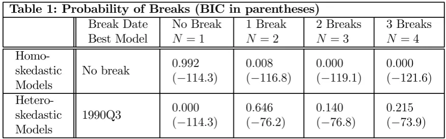
Table 1 presents evidence on structural breaks using the class of models defined in (3). The probabilities from the BMA exercises are shown for both homoskedastic and heteroskedastic (i.e. where the error variance changes when a break occurs) variants of our models.19
For the homoskedastic models there is less than one percent probability of any breaks. For the models with variance breaks, however, the BMA approach indicates most support for the one break model at around 65 percent. The probability of three breaks is just over 20 percent. Once heteroskedasticity is admitted, the probability of no breaks falls to zero.
Although we include the homoskedastic variants in our remaining empirical work, since they receive very little weight in our Bayesian model averaging exercises, we offer no further
discussion of them hereafter. Future references to particular models refer to the heteroskedas-tic versions.
The best model gives an estimated break date of 1990Q3, with a standard deviation of
1.71quarters. The point estimates of the error variance are0.29and0.02for the two regimes, indicating a greatly reduced error variance after 1990Q3. The two and three breaks models are also characterised by a substantial break in the error variance around 1990. For instance, three breaks yields estimated break dates of 1975Q2, 1983Q1 and 1990Q3, and a large reduction in the error variance after 1990Q3.20
Remember that we are treating, say, the two break model as a single model and integrat-ing out τ1 andτ2 using their posterior. For comparison, Table 1 also presents the BIC score
for the particular breakpoint(s) which yields the highest BIC . The one break heteroskedas-ticity model gives a maximum BIC of −76.2; and the corresponding three break model gives
−73.9. So the three break variant would be selected by a researcherfinding the values of the breakpoints which maximize the BIC (as opposed to integrating out these parameters).
[image:13.595.89.527.323.460.2]Overall, we conclude that the preliminary GDP(E) growth measurements became more accurate since 1990.
Table 1: Probability of Breaks (BIC in parentheses)
Break Date Best Model
No Break
N = 1
1 Break
N = 2
2 Breaks
N = 3
3 Breaks
N = 4
Homo-skedastic Models
No break 0.992
(−114.3)
0.008 (−116.8)
0.000 (−119.1)
0.000 (−121.6)
Hetero-skedastic Models
1990Q3 0.000
(−114.3)
0.646 (−76.2)
0.140 (−76.8)
0.215 (−73.9)
Notes: The probabilities are averaged over all possible threshold values. The number in paren-theses below the probability is the conventional BIC i.e. it is the BIC for the threshold value(s) which yield the highest BIC.
Researchers are often interested in whether the initial measurements exhibit unbiased-ness. That is, whether αj = βj = 0 for j = 1, .., N (i.e. whether unbiasedness occurs in
every regime). We can also calculate the probability of unbiasedness in the final regime as
p(αN =βN = 0|Data) (for the no breaks model αN =α andβN =β). Since this hypothesis
does not make sense for the regime-switching models, we exclude them from our calculations. The probability of unbiasedness at the end of the sample (averaged over the models with and without breaks) is1.000, indicating overwhelming evidence of unbiased preliminary measure-ments for the final regime. The earlier regimes do not share this property. Averaging across all regimes the probability of unbiasedness is 0.000.
The international evidence suggests that other countries exhibit bias with lengthy samples if structural breaks are not admitted. Faust, Rogers and Wright (2005) compared revisions for GDP growth across the G7 using OECD data. They found significant downward bias for
20Point estimates of the error variance in the four regimes are0.17,0.77,0.11 and 0.02, respectively. The
Germany, Italy, Japan and UK and less bias for Canada and the US.21 Garratt and Vahey
(2006) obtained similar results for UK data using a homoskedastic model.22 Faust, Rogers and Wright (2005) reported strong evidence of unbiasedness for the UK with post-1988 data. Thus, their UKfindings were consistent with our empirical results.
6.1.2 Evidence of Regime-Switching
Here we present the results for exogenous and endogenous regime switching in our models. Recall that exogenous switching uses the ECRI growth cycle dates for the UK and endogenous switching follows the form outlined in equation (4) section 3. For the endogenous switching models, we used threshold triggers of Zt =Xt, Zt =|Xt| andZt =Xt2 but we do not report
results forZt =|Xt| since the results are similar toZt=Xt2.23 Although we considered both
homoskedastic and heteroskedastic variants of the regime-switching models, homoskedasticity receives very little support so we report only for the heteroskedastic case.
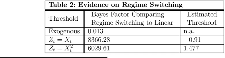
Table 2 presents Bayes factors comparing a regime switching model to the linear model with no breaks. Values of a Bayes factor greater than one indicate the regime switching model receives more support. For the exogenous regime switching models, the linear model receives the most support. However, the endogenous regime switching models do better. For instance, the regime-switching model withZt=Xt is over8,000 times as probable as the linear model.
Even then, the regime-switching models receive much less support than the structural break models discussed above. If we express the probabilities in Table 1 as Bayes factors, the model with one structural break is about1015times more likely than the linear models. Although we
include regime-switching models in our BMA forecasting exercises, they receive almost zero weight in the averaging and the subsequent discussion will emphasize the structural break models (with heteroskedasticity).
Notice that the model with the threshold definition Zt = Xt receives more support than
Zt = Xt2. There is little evidence that the volatility of output growth affects the revision
process.24 For the model with Z
t = Xt, the estimated threshold value indicates that, for
[image:14.595.75.466.536.637.2]very lowfirst measurements of GDP(E) growth (less than -1%), we get a high error variance; and for high values of the GDP(E) growth, we get a low error variance. Deep recessions are associated with less accurate data.
Table 2: Evidence on Regime Switching
Threshold Bayes Factor Comparing Regime Switching to Linear
Estimated Threshold Exogenous 0.013 n.a.
Zt=Xt 8366.28 −0.91
Zt=Xt2 6029.61 1.477
21See also the study by Croushore and Stark (2001) based on US National Accounts.
22Garratt and Vahey (2006) used the Bai and Perron (2003) methodology to test for breaks which is robust
to, but does not test for, breaks in the error variance. Their sample and definition of a revision differed from ours.
23The variable Z
t is used to divide the data into two parts based on the thresholdr. For the values ofr
supported by the data,Zt=Xt2 andZt=|Xt|do this division in a very similar manner.
24Mills and Wang (2003) estimate a structural break in output growth for 1993, more than four standard
In summary, the data indicate that the standard linear model does not provide an ade-quate description of the revisions process in GDP growth. The structural break models with breaks in the error variance are the ones which fit the data best. Regime-switching models receive more support than the standard linear model, but receive much less support than the structural break models.
6.2
Predicting Substantial Revisions
Since policymakers, statistical agencies and the press are interested in the probability of substantial GDP revisions in real time, we recursively estimate the models using data for 1961Q3 through to period t, where t=1984Q2, ..,2004Q1. For each of the 80 recursions, we calculate the one-step ahead event probability, p(|Yt+1| > a|Ω) whereΩ denotes information
available at the time of the first release of GDP growth and a = 0.3.25 Recall that this threshold defines substantial revisions as greater in absolute magnitude than the 2003Q2 revision. Since we average over all the models described (including linear, structural break and regime-switching models), and integrate out the parameters, our approach provides a formal treatment of model and parameter uncertainty.
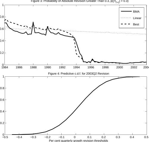
Figure 3 displays probability of revisions greater than 0.3 in absolute magnitude for BMA, the best model and the linear model with no breaks. Recall that all models are estimated recursively and that we treat break dates as parameters. So we define the best in each period as the model with the highest posterior probability. The best model varies over time, but always has structural breaks in the error variance. Typically the single break model is best, but at times the three break model has higher posterior probability.
Between 1986 and 1994, all three indicate probabilities between 0.45 and 0.7, with the BMA approach typically giving lower values than the linear model or the best model. Hence the BMA method highlights the risk that the other two models overstate the probability of substantial revisions early in the evaluation period. The BMA and best models indicate that the probability of substantial revisions was much lower after 1998 than before 1994. The posterior probability of a substantial revision fell sharply between 1994Q1 and 1995Q2, before levelling out at around 0.05. The probability for the linear model without breaks remained much higher, reaching around 0.5 by the end of the evaluation period.
There is some evidence that the probability of substantial revisions has increased slightly since 2001Q2 for the BMA and best models. Recall from figure 2 that a number of revisions greater than 0.2 in absolute value occurred just before the notorious 2003Q2 revision.
Since the focus of this paper is the probability of substantial revisions, it is the tails of the predictive that matter. However, the reader may be interested in the overall shape of the density so we provide the predictive cumulative density for the 2003Q2 revision obtained from our BMA exercise infigure 4. Given any threshold value aon the horizontal axis, the vertical axis gives the probability of a revision being less than a in 2003Q2 given the information set. That is, p(Y2003Q2 < a| Ω). For example, in our substantial revision exercise, we are
interested in the probability of the absolute revision being greater than 0.3%. To compute this probability we would need to use the probabilities associated with the -0.3% and 0.3%
25The working paper version, Garratt, Koop and Vahey (2006), reports additional results for alternative
thresholds, hence in this instance we would compute p(|Y2003Q2| > 0.3%| Ω) = p(Y2003Q2 < −0.3%| Ω) + [1−p(Y2003Q2 <0.3%|Ω)].
To help gauge forecasting performance of the BMA, best and linear models, we define a “correct forecast” as one wherep(|Yt+1|≤a|Ω)>0.5 and the observed revision is less than a or p(|Yt+1|> a| Ω)>0.5 and the observed revision is greater than a. (Remember that we
have calculatedp(|Yt+1|> a| Ω)for 80 periods, 1984Q3 to 2004Q2.) For a= 0.3, we observe
a high incidence of correct forecasts, sometimes referred to as the “hit rate”, using the BMA and best model approach of 74 percent and 69 percent, respectively. The linear model has a very low hit rate of only 19 percent.26
A more formal measure of forecast performance is the Pesaran and Timmermann (1992) directional market timing statistic, P T. As shown in Granger and Pesaran (2000), this hypothesis test uses the same information as the Kuipers score which measures the proportion growth rates greater than the threshold a that were correctly forecast minus the proportion of below mean growth rates that were incorrectly forecast. Under the null hypothesis that the forecasts and realisations are independently distributed the P T statistic has a standard normal distribution. For our substantial revision event, the data rejects the null of no ability to forecast observed changes, with values of 4.12 and 3.99 for the BMA and best models, respectively, and 0.84 for the linear model without breaks. The associated probability values are 0.00, 0.00 and 0.47, respectively. The no break linear model has a poor forecasting performance.
Thus, a strong message coming out of our analysis is that simply working with a lin-ear model yields misleading results. A second, weaker message, is that BMA offers some advantages over the strategy of simply choosing the single best model.
7
Conclusions
In this paper, we have shown that the probability of substantial revisions to UK GDP growth fell sharply after the 1980s, primarily as a result of a structural break in the error variance of revisions. We calculate that the probability of a revision of greater than the absolute magnitude of the 2003Q2 revision was around 1:20 in 2003. Using a wide set of models, including linear and nonlinear regression models with and without heteroskedasticity, we adopted a noninformative-prior Bayesian approach to produce the predictive distributions and forecasts of interests. In contrast, earlier classical econometric studies of revisions neglected formal analysis of model uncertainty and structural breaks in the error variances. Such an approach yields misleading predictives for our sample.
26Garratt, Koop and Vahey (2006) show that the three approaches have similar hit rates for smaller values
References
Akritidis L. (2003a). ‘Revisions to quarterly GDP growth’, Economic Trends, 594, pp. 94-101.
Akritidis L. (2003b). ‘Revisions to quarterly GDP growth and expenditure components’,
Economic Trends, 601, pp. 69-85.
Aruoba, B. (2005). ‘Data revisions are not well behaved’, mimeo, CIRANO Workshop on Data Revisions, October 2005, Montreal.
Bai, J. and Perron, P. (2003). ‘Computation and analysis of multiple structural change models’, Journal of Applied Econometrics, 18, pp. 1-22.
Castle, J. and Ellis, C. (2002). ‘Building a real-time database for GDP(E)’, Bank of England Quarterly Bulletin, February, pp. 42-49.
Charmokly, Z. and Soo, A. (2003) ‘The application of annual chain-linking to the Gross National Income System’,Economic Trends, 593, pp. 41-47.
Croushore, D. (2005) ‘An evaluation of inflation forecasts from surveys using real-time data’, mimeo, CIRANO Workshop on Data Revisions, October 2005, Montreal.
Croushore, D. and Stark, T. (2001). ‘A real-time data set for macroeconomists’, Journal of Econometrics, 105, pp. 111-130.
Diebold, F. X., and Rudebusch, G. D. (1991). ‘Forecasting output with the composite leading index: a real-time analysis’, Journal of the American Statistical Association, vol. 86, pp. 603-610.
Egginton, D., Pick, A, and Vahey, S. (2002). ‘ ‘Keep it real!’ A real-time UK macro data set’, Economics Letters, 77, pp.15-20.
Faust, J., Rogers, J. and Wright, J. (2005). ‘News and noise in G7 GDP announcements’,
Journal of Money, Credit and Banking, 37, pp. 403-420.
Fernandez, C., Ley, E. and Steel, M. (2001). ‘Benchmark priors for Bayesian model averaging’,Journal of Econometrics, 100, pp. 381-427.
Garratt, A. and Vahey, S.P. (2006). ‘UK Real-time data characteristics’, Economic Jour-nal, 116, F119-F135, February.
Garratt, A., Koop, G. and Vahey, S.P. (2006). ‘Forecasting substantial data revisions in the presence of model uncertainty’, RBNZ Discussion Paper 2006/02, March.
George, E. (2005). ‘Revisions to quarterly GDP growth and its production and expendi-ture components, Economic Trends, 614, pp. 30-39.
Granger, C. and Pesaran, M. (2000), ‘Economic and statistical measures of forecast accu-racy’,Journal of Forecasting, 19, pp. 537-560.
HM Treasury (1998). Statistics A Matter of Trust: A Consultation Document, The Sta-tionery Office, London.
Jenkinson, G. and George, E. (2005). ‘Publications of revision triangles on the National Statistics website’, Economic Trends, 614, pp. 43-44.
Koop, G. (2003). Bayesian Econometrics, John Wiley and Sons, Chichester.
Koop, G. and Potter, S. (2003). ‘Bayesian analysis of endogenous delay threshold models’,
Journal of Business and Economic Statistics, 21, pp. 93-103.
Koop, G. and Potter, S. (2001). ‘Are parent findings of nonlinearity due to structural instability in economic time series?’, The Econometrics Journal, 4, pp. 37-55.
Koop, G. and Potter, S. (1998). ‘Bayes factors and nonlinearity: evidence from economic time series’, Journal of Econometrics, 88, pp. 251-281.
Lawson, N. (1992). The View From No. 11: Memoirs of a Tory Radical, Bantam Press, London.
Mankiw, N.G., Runkle, D. and Shapiro, M.(1984). ‘Are preliminary announcements of the money stock rational forecasts’, Journal of Monetary Economics, 14, pp. 15-27.
McConnell, M. and Perez, G. (2000). ‘Output fluctuations in the United States: What has changed since the early 1980s?’, American Economic Review. 90, pp. 1464-76.
Mills, T. and Wang, P. (2003). ‘Have output growth rates stabilised? Evidence from the G-7 economies’, Scottish Journal of Political Economy, 50, pp. 232-246.
National Statistics (2005). Code of Practice; Protocol on Revisions, The Stationery Office, London.
Office for National Statistics. Economic Trends, various issues, The Stationery Office, London.
Office for National Statistics. Economic Trends Annual Supplement, various issues, The Stationery Office, London.
Osborn, D. and Sensier, M. (2002). ‘The prediction of business cycle phases: financial variables and international linkages’,National Institute Economic Review, October.
Pesaran, M. and Timmermann, A. (1992). ‘A simple nonparametric test of predictive performance’, Journal of Business and Economic Statistics, 10, pp. 461-465.
Patterson, K. and Heravi, M. (1991). ‘Data revisions and the expenditure components of GDP’, Economic Journal, 101, pp. 887-901.
Richardson, C. (2003). ‘A time series approach to revisions’, Economic Trends, 601, pp. 86-89.
Robinson, H. (2005). ‘Revisions to quarterly GDP growth and its production (output), expenditure and income components’, Economic Trends,625, pp. 34-49.
Schwarz, G. (1978). ‘Estimating the dimension of a model’, Annals of Statistics, 6, pp. 461-464.
Statistical Commission (2004). Revisions to Economic Statistics, Report no 17, Vol. 1,2 and 3, April. The Mitchell Report.
Statistical Commission (2005). Official Statistics: Perceptions and Trust, Report no. 24, London.
Stock J. and Watson, M. (2002). ‘Has the business cycle changed and why?’, NBER Macroeconomic Annual.
Swanson, N. and van Dijk, D. (2006). ‘Are statistical reporting agencies getting it right? Data rationality and business cycle asymmetry’,Journal of Business and Economic Statistics, 24, pp. 24-42.
Symons, P. (2001). ‘Revisions analysis of initial estimates of annual constant price GDP and its components’, Economic Trends, 568, pp. 48-65.
1961 1965 1970 1975 1980 1985 1990 1995 2000 2005 −5
[image:19.595.23.572.188.670.2]−4 −3 −2 −1 0 1 2 3 4 5 6
Figure 1: First and Second GDP Quarterly Growth Measurements, 1961Q3 − 2004Q2
1980 1984 1988 1992 1996 2000 2005 −1
−0.8 −0.6 −0.4 −0.2 0 0.2 0.4 0.6 0.8 1
Figure 2: GDP Quarterly Growth Revisions, 1980Q1 − 2004Q2
First Second
2003Q2
−0.50 −0.4 −0.3 −0.2 −0.1 0 0.1 0.2 0.3 0.4 0.5 0.2
0.4 0.6 0.8 1
Figure 4: Predictive c.d.f. for 2003Q2 Revision
Per cent quarterly growth revision thresholds
19840 1986 1988 1990 1992 1994 1996 1998 2000 2002 2004 0.2
[image:20.595.47.547.184.660.2]0.4 0.6 0.8 1
Figure 3: Probability of Absolute Revision Greater Than 0.3, p(|YT+1| > 0.3)
BMA
Linear