BIROn - Birkbeck Institutional Research Online
Collins, E.J. and Brooms, Anthony C. (2005) The Bernoulli Feedback Queue
with Balking: stochastic order results and equilibrium joining rules. Working
Paper. Birkbeck, University of London, London, UK.
Downloaded from:
Usage Guidelines:
Please refer to usage guidelines at or alternatively
ISSN 1745-8587
Birkbeck Workin
g
Pa
p
ers in Economics & Finance
School of Economics, Mathematics and Statistics
BWPEF 0517
The Bernoulli Feedback Queue with
Balking: Stochastic Order Results
and Equilibrium Joining Rules
E.J. Collins
A.C. Brooms
The Bernoulli Feedback Queue with Balking:
Stochastic Order Results and Equilibrium Joining
Rules
E. J. Collins
∗A. C. Brooms
†7 November, 2005
Abstract
We consider customer joining behaviour for a system that consists of a FCFS queue with Bernoulli feedback. A consequence of the feedback characteristic is that the sojourn time of a customer already in the system depends on the joining decisions taken by future arrivals to the system. By establishing stochastic order results for coupled versions of the system, we prove the existence, and unique-ness, of Nash equilibrium joining policies, and show that these are characterized by (possibly randomized) threshold rules. We contrast the Nash rule with the socially optimizing joining rule that minimizes the long-term expected average sojourn time (or cost) per customer. The latter rule is characterized by a non-randomized threshold, and we show that the Nash rule admits at least as many customers into the system as the socially optimizing one.
Keywords: FCFS queue with Bernoulli feedback; coupling; Nash equilibrium; social optimality
AMS: 90B22; 91A10; 60E15; 91A13; 91A14
1
Introduction
This paper considers the joining behaviour of customers into a First Come First Served Bernoulli Feedback queueing system. Each arriving customer joins the system, or balks, on the basis of the number of customers already present. It is assumed that cus-tomers who join the system do not renege at any stage. An important consequence of the Bernoulli feedback property is that the sojourn time of any customer who is already
∗Department of Mathematics, University of Bristol, University Walk, Bristol BS8 1TW, U.K. †School of Economics, Mathematics, & Statistics, Birkbeck College, Malet Street, London WC1E
in the system may be affected by customer arrivals in the future. Joining behaviour of customers to the system is considered in the context of the following two scenarios. In the first, each customer compares their expected sojourn time (or cost) in the sys-tem with some fixed cost parameter associated with balking, and makes the joining decision that yields the smallest expected cost. Since this involves taking into account the joining decisions taken by other customers, it is natural to consider the Nash equi-librium as the appropriate characterization of behaviour. Our second scenario is one in which the joining decision of each customer is selected by a centralized authority, with the objective of minimizing long-term expected costs averaged across all cus-tomers. In common with other literature on admission control into queues, we discuss whether decentralized decision making can be as good as, or perhaps worse than, that under centralized control, when judged according to the social criterion posed in our problem.
Naor (1969) carried out one of the earliest studies of optimal customer joining behaviour into single-server queueing systems. He assumes a constant holding cost per customer per unit time and assumes that a fixed reward accrued to each customer in the system upon completion of service (thus, in effect, a linear holding cost). He shows that, within the class of (stationary) deterministic threshold policies, there exist unique individually optimal and socially optimal joining rules that minimize the expected cost to each customer and the long-run (expected) cost per unit time, respectively. Finally, he also shows that the socially optimal threshold is a lower bound on the threshold that is individually optimal.
Similar results have been established in a number of extensions to the above sys-tem. For example, Yechiali (1971) considers the GI/M/1 system (with linear cost struc-ture), and shows that, amongst all policies, there exists a non-randomized threshold joining rule that is self-optimizing, from the point of view of each customer. He also shows that in the class of stationary policies, the socially optimizing policy that mini-mizes an average cost criterion, is also characterized by a non-randomized threshold. Again the socially optimal threshold is seen to be a lower bound to the one that is individually optimal. Yechiali (1972) establishes corresponding results for the GI/M/s queue. However, Altman & Hassin (2002) argue that the individually optimal joining policy for theM/G/1queue does not exhibit the usual threshold structure, due to the queue lengths giving an indication as to the residual time of the customer in service to new arrivals at the system.
arrivals. This allows policies to be formulated that are optimal for each individual cus-tomer. However, in feedback models, the sojourn time of a customer already in the system depends on the joining decisions taken by future arrivals to the system. Nat-ural applications of FCFS queueing systems with feedback arise, for example, in the theory of telephone traffic (Tak´acs 1963); see Takagi (1991) and the references therein for variations and extensions to the basic model. We can also think of this system as a model for a single-line manufacturing process in which each job is independently tested, and sent through the process again if a fault is discovered or the work done to the job is deemed unsatisfactory (Pek¨oz & Joglekar 2002). We can still define and con-struct ’optimal’ joining rules for these models, but only if knowledge about the joining behaviour of future arrivals can be assumed; thus the appropriate solution concept to consider is that of the Nash equilibrium, and we discuss this in detail later in this paper. Nash equilibrium joining rules for a ’single line’ queueing system have been exam-ined by Altman & Shimkin (1998) in the context of the processor sharing discipline. There it was assumed that the effective service rate to each customer in the queue,
ν(x) = µ(x)/x, is strictly decreasing in x(wherexis the number in the system, and
µ(x)the corresponding service rate). For their system, they show that any candidate Nash equilibrium policy is characterized by a threshold structure, that a Nash equilib-rium policy always exists, and will be unique when the policy is symmetric, i.e. each customer invokes exactly the same joining rule. This model was later extended to the case of multi-class heterogeneous preferences in Ben-Shahar, Orda & Shimkin (2000), in which the existence of the Nash equilibrium was also established.
The analysis of Altman & Shimkin (1998) can be modified and extended to deal with the multiple-server retrial queue (Brooms 2000), and the FCFS queue where the service rate is (strictly) decreasing in the number in the system (Brooms 2003). More recently, the FCFS queue with service rate strictly increasing in the queue length was analyzed in Brooms (2005). It was shown that, under the proviso that the joining rule for each customer is such that the chance that they are admitted to the queue is a non-increasing function of the queue length, there exists (at most) a finite number of symmetric Nash equilibria, and that at least one of these does not invoke randomization in its joining decisions. This should be contrasted with Altman & Shimkin (1998) in which existence and uniqueness were established (but with no guarantee of it being non-randomized) within the widest possible class of policies.
coupling used, ’dominance’ across each and every pair of realizations is not achieved. So, in addition to the game-theoretic results presented in this paper, our second main contribution arises from the construction and use of apparently novel couplings in order to prove the ancillary lemmas.
The rest of this paper is organized as follows. In Section 2, the formulation of our model, a prescription of the joining rules to be used by customers, and a summary of the main results, are presented. In Section 3, sample path comparisons for our queue-ing process, and monotonicity results for the expected sojourn time in the system, as a function of the entry queue lengthx, are established. Similar results are proved with respect to the threshold value associated with symmetric threshold joining policies in Section 4; we also prove a continuity result for the expected sojourn time with respect to this threshold. We bring these results together to characterize the structure, and to prove the existence and uniqueness of a certain symmetric Nash equilibrium joining policy in Section 5. We also show that a certain socially optimizing policy can be characterized by a non-randomized threshold, and show that this is, in fact, a lower bound on the Nash threshold. We close the paper in Section 6, with some concluding remarks.
2
Preliminaries
2.1
The model
Consider a service system consisting of a single server queue (denoted by Q) with Bernoulli Feedback and First Come First Served (FCFS) queue discipline. Assume that each arriving customer joins the queue with a probability that depends only on the observed queue lengthx in Qjust prior to their arrival at the system, and allow randomized decisions. A joining rule for an arriving customer is thus a sequence of numbers{u(x)∈[0,1] : x= 0,1,2. . . , B−1}, whereB may be finite, or infinite; if the queue length just prior to their arrival isxthen the customer joins the system with probabilityu(x)and otherwise balks (i.e. does not join).
More formally, consider a process that starts at timet = 0with an arriving customer
C0 that joins Q. We denote the subsequent arriving customers byC1, C2, . . . and let
X(t)denote the number of customers inQat timet, with initial stateX(0) =x0.
Let T = {T1, T2, T3, . . .} denote a sequence of independent, identically distributed,
positive, continuous random variables, with finite expectation, which we interpret as the successive inter-arrival times, and let W = {W1, W2, W3, . . .}, and W, denote
a sequence of independent, identically distributed, positive, continuous random vari-ables, with finite expectation, which we interpret as the successive service times. The arrival epochs (to the system) of successive customersC1, C2, C3, . . . are then given
and, at least until the queue is empty for the first time, the successive service com-pletion epochs inQare given by the sequenceS = {S0, S1, S2, S3, . . .}, whereSk =
S0 +W1 +· · ·+Wk, k = 1,2, . . . (with appropriate modification thereafter). We assume that, with probability 1, the arrival epochs and service completion epochs are distinct.
Similarly, let U = {U1, U2, U3, . . .} denote a sequence of independent random
vari-ables, each of which has a uniform distribution on the interval (0,1] and let F = {F0, F1, F2, . . .} be a sequence of independent Bernoulli random variables with
pa-rameter p, so for each k = 0,1,2,3, . . ., Fk = 1 with probability p ∈ (0,1) and
Fk = 0with probability1−p. We interpret theU’s as the successive arrival joining decision variables, so customerCk joinsQif and only ifUk ≤uk(X(Ak)), and inter-pret theF’s as the successive feedback decision variables, so at the completion of the
j-th service inQafter timet = 0, the customer that has just completed service is fed back to the end of the queue inQifFj = 1and otherwise departs the system ifFj = 0.
In an abuse of terminology, we shall sometimes useQto refer to the process as well as the queueing system itself; we shall refer to the number held in the system as the queue size or length (thus referring to the total number of customers queueing up for, and actually in, service). Under this model, the evolution ofQ is completely deter-mined by the initial queue sizeX(0), the collection of joining rules for each one of the future customers{u1, u2, . . .}, the residual service timeS0 of the customer (if any) in
service atQatt= 0, and the values of the variables in the sequencesT,W,U andF. In particular, we assume{X(t) :t ≥ 0}is a left-continuous, piecewise constant pro-cess, whose jumps, if any, occur at arrival epochs{Ak}or service completion epochs {Sj}, so that atSj a customer is still with the server, whereas at Sj+ the customer has either left the system or been fed back to the end of the queue. The jumps are formally described by the relations:
X(A+k) = X(Ak) +1{Uk ≤uk(X(Ak))} k = 1,2,3, . . . (1)
X(S+
j ) = X(Sj)−1{Fj = 0} j = 0,1,2, . . . (2) with appropriate modification if the buffer is full, orX(Sj) = 0,j = 0,1,2, . . ..
2.2
Individual joining rules and population policies
For nonnegative integerL ∈Nandq ∈[0,1), we say a joining ruleuis an[L, q] -threshold rule if forx∈N
u(x) =
1 if x < L q if x=L
0 if x > L
(3)
Associated with each[L, q]-threshold rule is a unique real valueg =L+q. We refer tog as the threshold value associated with the rule, and represent the rule itself more compactly by[g].
For a population of customers arriving in the sequence C0, C1, C2, . . ., we call the
corresponding vector of customer joining rules a population joining policy and denote it by π = (u0, u1, u2, . . .). We letD∞ denote the class of non-increasing population
policies for which each component ruleuk is such that uk(x)is non-increasing in x; we let S∞ denote the class of symmetric population policies for which each of the components rulesuk are identical; and we letT∞denote the class of threshold popu-lation policies, for which eachukis a threshold joining rule. Observe thatT∞ ⊂D∞. If all customers adopt the same joining rule u then we denote the resulting popula-tion joining policyπ = (u, u, u, . . .) ∈ S∞ byu∞; similarly, if all customers use the same threshold joining rule [g]we denote the resulting population joining policy by
π= [g]∞.
2.3
Main Results
In the following sections, we prove a number of stochastic order results pertaining to the behaviour of the expected sojourn time of a customer in the system. Apart from being of interest in their own right, these results will be used to establish the existence, uniqueness, and structure of Nash equilibrium population joining policies for an asso-ciated stationary game.
Letvk(x, β, π),x∈N,be the sojourn time ofCk inQ, given that at its arrival,x cus-tomers were already present in the system, the residual service time of the customer at the server isβ > 0, and that future arrivals adhere to the decision rules inferred by
π. Define Vk(x, β, π)to be the expected value of vk(x, β, π). When the service time has an exponential distribution, the expected sojourn time of a customer that joins the queue does not depend on the residual service time (if any), and we simply write
vk(x, π)andVk(x, π)respectively.
Note: indexing of entry queue sizes of the formx ∈ N,x = 0,1, . . ., orx = 1,2, . . . are to be understood as running up toB −1wheneverB is finite. Also, the interval [0, B)is interpreted to mean[0, B]ifBis finite, and[0,∞)ifB is infinite.
the dependence of the expected sojourn time on bothxandg, and are mostly proved by invoking couplings of a non-trivial nature. The game-theoretic results of Theorems 5 and 6 are proved using a combination of Theorems 1-4, but under the proviso that the total expected time spent at the server for a customer inQis less than the ’cost’ of balking from the system.
Theorem 1 Consider aGI/G/1Bernoulli feedback system and let π ∈ D∞ be any non-increasing population joining policy. Then, for each x = 1,2, . . . and β > 0,
V(x+ 1, β, π)−V(x, β, π)≥(1−p)E(W).
The specialization of this result to the case of exponential service times can be found in Corollary 3.1. Theorem 1 is somewhat less general than its counterpart in Altman & Shimkin (1998) in thatπ is restricted to lie inD∞. The classD∞ infers that there is less chance that each customer actually joins the system as the queue length there increases. Under additional assumptions on the arrival and departure processes, we can extend our result to another class of policies.
Theorem 2 Consider anM/M/1Bernoulli feedback system and letπ ∈ S∞be any symmetric population joining policy. Then, for eachx = 0,1,2, . . ., V(x+ 1, π)−
V(x, π)≥(1−p)E(W).
Theorem 3 Consider aGI/G/1Bernoulli feedback system and let[g]∞and[eg]∞be symmetric threshold population joining policies with0≤g <egandeg ∈[0, B). (i) Suppose eg ≤ 1. Then V(0,[eg]∞) = V(0,[g]∞), and for each x = 1,2, . . . and
β >0,V(x, β,[eg]∞) =V(x, β,[g]∞).
(ii) Supposeg ≥1. Then there existsδ0 >0such thatV(0,[eg]∞)−V(0,[g]∞)≥ δ0,
and for each x = 1,2, . . . and β > 0, there exists δx > 0such that V(x, β,[eg]∞)−
V(x, β,[g]∞)≥δx.
Theorem 4 Consider aGI/G/1Bernoulli feedback system and let[g]∞be a symmet-ric threshold population joining policy withg > 0. ThenV(0,[g]∞) is a continuous function ofg, and, for each x = 1,2, . . . and β > 0, V(x, β,[g]∞) is a continuous function ofg ∈[0, B).
Theorem 5 Consider aGI/M/1Bernoulli feedback system and assume that attention is restricted to the classD∞of non-increasing population joining policies.
(i) Ifπ = (u0, u1, u2, . . . , . . .)∈ D∞is a Nash equilibrium population joining policy,
then eachukis a threshold joining rule (with finite threshold).
(ii) There exists a unique symmetric Nash equilibrium population joining policyπ∗ = (g∗, g∗, g∗, . . .) = [g∗]∞in the class of policiesD∞.
Theorem 6 Consider anM/M/1Bernoulli feedback system.
(i) If π = u∞ ∈ S∞ is a Nash equilibrium population joining policy, then u is a threshold joining rule (with finite threshold).
3
Monotonicity in the queue length x
3.1
Monotonicity for a GI/G/1 system
We first consider aGI/G/1Bernoulli feedback queueing system where each potential customer uses a joining rule which is a non-increasing function of the queue size just prior to their arrival. Let x denote the queue size upon joining. We show that, for
x≥1, the expected sojourn time of a joining customer is a strictly increasing function ofx.
Without loss of generality, we focus on a marked customer C that joins the queue at time t = 0. For k = 1,2,3, . . . , , we assume each successive potential customer,
Ck, say, arrives at corresponding epochAk, and finds a queue of size X(Ak). Ckhas the option of either joining the queue or departing the system, and joins the queue with probabilityuk(X(Ak)), where eachuk(x)is a (possibly different) non-increasing function ofx. Note that the presence of a finite bufferBcan be incorporated by taking
uk(x) = 0forx≥B.
Letv(x, β, π)denote the sojourn time for customerC who joins the queueing system, when the queue size just prior to arrival isx ≥ 1, the population joining policy (i.e. the set of joining rules for later arriving potential customers) isπ = (u1, u2, u3. . . . ,),
and when the residual service time for the customer currently in service at timet = 0 isS0 =β >0. LetV(x, β, π)be the expected value of this quantity.
To comparev(x, β, π)withv(x+ 1, β, π), we look at path-wise comparisons of cou-pled realizations of two queueing processes, sayQandQe, in which marked customers
C (resp. Ce) join the queue at timet = 0when there are alreadyx(resp. x+ 1) cus-tomers in the queue, the population joining policy isπand the current residual service time isβ. We say that at each timeta customer in theQprocess is level with a cus-tomer in theQeprocess if both have the same position (first, second, third etc.,) in their respective queues, and we say one customer is ahead of (resp. behind) the other if it has a position nearer (resp. further from) its server. We show that for each sample path in the coupled processes, the customer who joins withxin the system leaves either at the same epoch or at least one service completion before the customer who joins with
x+ 1in the system. Moreover, this second possibility happens on a set of positive probability, so thatV(x, β, π)< V(x+ 1, β, π).
Coupling 1 (i) Consider two processesQ and Qe with X(0) = x > 0 andXe(0) =
y > 0. Couple the systems so that they have the same initial residual lifetime and so that, taken in the natural order, they have the same sequence of inter-arrival times, the same sequence of service times, the arriving customers use the same sequence of join-ing rules and the joinjoin-ing decision random variables take the same sequence of values. Formally, this means we setS0 =Se0 =β,T =Te,W =Wf,π =eπandU =Ue.
(ii) Now couple the feedback decision variables as follows. Forr = 1,2,3letFr = {Fr,1, Fr,2, Fr,3. . .}denote mutually independent sequences of independent Bernoulli
random variables, each with parameterp.
Use the sequence of values in F1 to determine both the successive feedback
deci-sions for customerC inQ and the successive feedback decisions forCe inQe, so, for example, bothC andCe are fed back after their first service if and only if F1,1 ≤ p.
Thus bothC andCeare fed back exactly the same number of times in both processes.
Use the sequence of values inF2to determine the successive feedback decisions for all
other customers inQ. Thus, the first customer inQother thanC to complete service is fed back if and only ifF2,1 ≤p, the second is fed back if and only ifF2,2 ≤p, etc.
Now consider the other customers in Qe. By construction, the two processes Q and
e
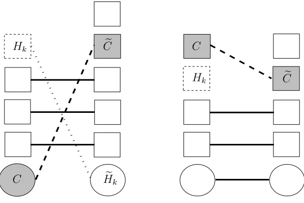
Qhave the same service completion epochs, at least until one or other is empty for the first time. During this period, couple the feedback decision for each customer other thanCe to be exactly the same as that for the corresponding customer completing at the same time inQ, except for customers (other thanCe) who complete service at the same time asC. Say there is such a customer who completes service inQeat the same moment thatC completes itsk-th service inQ. Denote this customer by Hek and de-note byHk that customer inQ(if any) which is level withCeat that moment. If such a customer Hk exists, define the the feedback decision for Hek to be the same as the (already assigned) next feedback decision forHk in Q. If there is no customer level withCe at that moment, then define the feedback decision for Hek using the value of thek-th variable in the sequenceF3. Once the two processes no longer have the same
service completion epochs, the feedback decisions can be assigned arbitrarily. ¤
Note that under Coupling 1 a customer oppositeC may depart even though C is fed back, so there may be epochs s when X(s) > Xe(s). As well as showing how the relative positions ofCandCeare maintained between their service completion epochs, the next Lemma shows that ifXe(0) =X(0) + 1thenX(s)can never exceedXe(s) + 1.
C Hek
e
C Hk
Hk
C
e
[image:12.595.137.446.108.314.2]C
Figure 1: A possible realization ofQandQejust prior (L.H.S.) and just after (R.H.S.)
C is fed back for thek-th time. C andHek are in service on the L.H.S. The feedback decisions for C and Ce remain coupled throughout. The feedback decision for Hek is coupled with that ofHk ifHkis present, otherwise it is chosen independently; in the diagram neither are fed back. The next feedback decisions for the other customers in
e
Qare coupled with those for the parallel customers inQ, and will be reassigned if they are fed back.
τ∪ {0}. Then
(i) The positions ofCandCerelative to each other do not change in(s, t). (ii) IfXe(s+)≥X(s+)thenXe(t)≥X(t).
(iii) IfX(s+) = Xe(s+) + 1thenX(t)≤Xe(t) + 1.
Proof
Consider the processes in the interval(s, t), where any feedback decisions following the first service completion have been implemented by times+, but those following the second service completion have not yet been implemented at t (by virtue of the ’left-continuity’ of the queue-length process). During the interval, the composition of each queue changes only at arrival or service completion epochs.
(i): At service completion epochs, the coupling ensures that customers make the same feedback decision in both processes, so the positions ofCandCerelative to each other do not change. At arrival epochs, the arriving customers join behind C and Ce, so cannot affect their relative positions until the next epoch inτ. Thus the positions ofC andCerelative to each other do not change in(s, t).
taken in both processes. At arrival epochs when one queue is smaller than the other, the fact that the joining decision rule is a non-increasing function of the size of the queue, together with the coupling and relation (1), ensures that either the same joining decision is taken in both processes or the arrival joins the queue in the process with the smaller queue but does not join in the process with the larger queue. Thus the difference in the queue sizes can only decrease during(s, t)and once the queue sizes are equal, they remain equal. In particular, ifX(s+) =Xe(s+) + 1then eitherX(t) =
e
X(t)orX(t) =Xe(t) + 1, so in either caseX(t)≤Xe(t) + 1. ¤
Lemma 3.2 Consider realizations of the two processes Q and Qe under Coupling 1 withy = x+ 1, and assume the population follows some non-increasing population policyπ ∈ D∞. Let K denote the common number of visits bothC andCe make to the server in each realization, and let s1, . . . , sK and es1, . . . ,esK denote the service completion epochs forC andCerespectively. Then Xe(sk) ≥ X(sk)andesk ≥ sk for
k= 1, . . . , K.
Proof
Fork= 1, . . . , K, letPkdenote the proposition: Xe(sk)≥X(sk)andesk ≥sk.
First assume K = 1. At t = 0+, C has x other customers ahead of it in Q while
e
Chasx+ 1customers ahead of it inQe, so the position ofCinQis one ahead of that ofCeinQe. From Lemma 3.1, these relative positions are maintained untilCcompletes service, soCleaves the system exactly one service completion epoch beforeCe. More-over,Xe(0+) = X(0+) + 1> X(0+)so again from Lemma 3.1Xe(s1)≥X(s1). Thus
P1 is true.
Now assume Pk is true for some k = 1, . . . , K − 1 for K > 1. Since k < K, bothC andCe are fed back after their k-th service. NowC is either level with Ce at
sk orC is ahead ofCe atsk. IfC is ahead ofCe atsk, then there may or may not be a customer inQlevel withCeatsk. If there is a customer in Qlevel withCe atsk, then that customer may or may not be fed back at its next service. There are then four cases to consider.
Case 1: [C is level withCeatsk].
SinceCis level with Ce atsk andesk ≥ sk, bothC andCeare fed back together atsk. SinceXe(sk) ≥ X(sk)and C was fed back withCeat sk, C is level with or ahead of
e
C after being fed back, andXe(s+k) ≥ X(s+k). Lemma 3.1 then implies that the next epoch inτ occurs at sk+1, that C is still either level with or ahead ofCe at that point
and thatXe(sk+1)≥X(sk+1). Finally,Cehad completed no more thankservices ats+k
so it must have completed no more thank+ 1services ats+k+1, soesk+1 ≥sk+1.
Case 2: [C is ahead ofCeatskand there is no customer inQoppositeCeatsk].
follows immediately that: (i)Xe(sk) > X(sk), (ii) C must be level with or ahead of
e
Cafter being fed back, and (iii) the feedback decision for the customerHek inQewho completes service atsk is determined by the corresponding value in the sequenceF3,
independent of the realization forQ. SinceXe(sk)> X(sk), we haveXe(s+k)≥X(s+k) whetherHekdeparts or is fed back. SinceC is level with or ahead ofCe ats+k, Lemma 3.1 implies that the next epoch inτis atsk+1, thatCis still level with or ahead ofCeat
that point, and thatXe(sk+1)≥ X(sk+1). SinceC was ahead of Ceatskandesk ≥ sk,
e
C must have completed at least one less service than C at s+k, so it must still have completed at least one less service thanCats+k+1, givingesk+1 > sk+1.
Case 3: [C is ahead of Ce at sk, Hk is opposite Ce at sk and is fed back at its next service].
Since C is ahead of Ce at sk then, together with sek > sk, this implies that Ce must have completed say(r−1)services at s+k, where(r−1) < k. SinceC is ahead of
e
C at sk, there is a customer Hek =6 Ce in Qe who completes service atsk and whose feedback decision is coupled to be the same as that forHk, i.e.Hek is also fed back at
s+
k. ThusXe(s+k) ≥ X(s+k). Since there was a customer level withCe atsk, C is now behindCeafter the feedback. Lemma 3.1 then implies that the next epoch inτ occurs whenCe completes service at ser and that Xe(esr) ≥ X(esr). At es+r, Ce has completed
r ≤ k < K services, so bothCeandHkare fed back, givingXe(es+r)≥ X(es+r). Since
e
X(ser)≥X(esr),Cis now ahead ofCeafter the feedback. Lemma 3.1 then implies that the next epoch inτ occurs whenC completes service atsk+1, thatC is still ahead of
e
Cat that point, and thatXe(sk+1) ≥X(sk+1). SinceCehad completedr ≤ kservices
ates+r and has not completed any more services bysk+1, we haveesk+1 > sk+1.
Case 4: [C is ahead of Ce at sk, Hk is opposite Ce at sk and departs at its next ser-vice].
Since Hek now departs at sk while C is fed back, we have X(s+k) ≤ Xe(s+k) + 1so eitherX(s+k) ≤ Xe(s+k) or X(s+k) = Xe(s+k) + 1. Since there was a customer level withCe at sk, C is now behind Ce after the feedback. Letr be as in Case 3. Lemma 3.1 now implies that the next epoch inτ occurs whenCecompletes service atser, and thatX(esr) ≤ Xe(ser) + 1, so either X(esr) ≤ Xe(esr)or X(esr) = Xe(ser) + 1. Ates+r,
e
C has completedr ≤ k < K services and so is fed back, whileHk departs just like
e
Hk, so eitherX(es+r) ≤ Xe(es+r)−1orX(esr+) = Xe(se+r), i.e.Xe(es+r) ≥ X(es+r). Thus
e
C is either fed back level withC or behindC. Lemma 3.1 now implies that the next epoch in τ is at sk+1, thatC is still level with or ahead of Ce at that point, and that
e
X(sk+1) ≥ X(sk+1). SinceCe had completed less thank services ats+k and has only completed one service betweensk andsk+1, it has completed at most k+ 1services
bys+k+1, and soesk+1 ≥sk+1.
establishingP1 whenK = 1), the result follows by induction. ¤
Theorem 1
Consider aGI/G/1Bernoulli feedback system and letπ ∈D∞be any non-increasing population joining policy. Then, for eachx = 1,2, . . . andβ > 0, V(x+ 1, β, π)−
V(x, β, π)≥(1−p)E(W).
Proof
Consider realizations of the two processesQ and Qe as in Coupling 1. Assume that there are initiallyxcustomers ahead ofCinQandy=x+ 1customers ahead ofCein
e
Qand that customers in bothQ andQe are using the same non-increasing population joining policy π ∈ D∞. From Lemma 3.2, C completes its first service at s1 (one
customer ahead ofCe), and completes all its remaining services either level withCeor at least one customer ahead. The probability thatC (andCe) depart after just one service is(1−p), and the expected extra time Ce spends inQe in that case is E(W). Thus, taking expectation over all possible realizations, we haveV(x+1, β, π)−V(x, β, π)≥
(1−p)E(W). ¤
3.2
Monotonicity for a GI/M/1 system
When the service time has an exponential distribution, the residual service time of a customer in service at an arrival epoch has exactly the same exponential distribution as the service time of a customer starting service at that point. Thus the expected sojourn time of a customer that joins the queue does not depend on the residual service time of the customer (if any) in service on joining. In this case we can writeV(x, π)for the expected sojourn time for customerC when the queue size on joining isxand the population joining policy isπ= (u1, u2, u3. . . .).
Corollary 3.1
Consider aGI/M/1Bernoulli feedback system and letπ ∈D∞be any non-increasing population joining policy. Then, for eachx = 0,1,2, . . ., V(x+ 1, π)−V(x, π) ≥ (1−p)E(W).
Proof
The proof forx= 1,2, . . .follows directly from Theorem 1 since the expected sojourn times are independent ofβ. Moreover, the result forx = 0can be proved in exactly the same way as the results for x > 0in section 3.1, since we can now arrange the coupling so that the residual service time of the customer in service inQeatt = 0has exactly the same value as the service time of the customer joining and entering service
3.3
Monotonicity for an M/M/1 system
When the arrival process forms a stationary Poisson process we can extend the class of population joining rules for which Theorem 1 applies. Consider anM/M/1Bernoulli feedback system where potential customers all use the same joining ruleu, whereu(x) is a general (not necessarily non-increasing) function of the queue sizexon arrival. We again show that the expected sojourn time of a customer that joins a non-empty queue is a strictly increasing function of the queue size on joining.
Again let v(x, π) denote the sojourn time for customer C when the queue size on joining isx≥1, when the symmetric population joining policy (for arriving potential customers) isπ = u∞, and let V(x, π)be the expectation of this quantity. Again we compare v(x, π) with v(x+ 1, π), by looking at path-wise comparisons of coupled realizations of two queueing processes, sayQ andQe, in which marked customersC (resp. Ce) join the queue att = 0when there are alreadyx(resp. x+ 1) customers in the queue.
The coupling we use is, perhaps, more complex than Coupling 1, but is again de-signed to ensure that bothCandCemake the same number of visits to the server in the coupled systems.
For fixedu, the evolution of Qe is completely specified as before by the sequence of successive inter-arrival timesTe, service timesWf, joining decision random variablesUe and feedback random variablesFe. The coupled evolution ofQcan then be described informally as follows: Consider a realization ofQe in whichCe makesK visits to the server. For k = 1,2,3, . . . let es1, . . . ,esK denote the corresponding service comple-tion epochs ofCe. We ”freeze” the processQuntilCeis level with Cand then couple the two processes to have the same arrival epochs, service completion epochs, arrival decision variables and feedback decision variables until bothC andCe complete their first service. By construction, whenCe is fed back for the first time, there are at least as many customers ahead of it as there are ahead ofC when it is fed back for the first time. To extend the realization until the next service completion epoch forC, again ”freeze” the processQuntilCeis again level withCand then re-couple them until both
CandCecomplete their next service. This procedure can be continued iteratively until bothCandCedepart.
We can define this coupling more formally as follows:
Coupling 2
Let s1, . . . , sK and es1, . . . ,esK be the successive service completion epochs of cus-tomersC andCe, respectively, and set s0 = es0:= 0. For somek ∈ {0, . . . , K −1},
assume that we have constructedQup to the epochs+k,Xe(esk)≥X(sk)andesk≥sk.
rep-resents the difference between the number ahead ofCand the number ahead ofCeas they are fed back for thek-th time (resp. as they join their respective systems at time0).
Now observe Qe from es+k until b services have taken place and then couple Q with it. Letr1, r2, . . . denote the arrival epochs of successive customers inCeafter esk and
t1, t2, . . . the successive service completion epochs. Assume that there have been e
arrivals and f services in Qe prior to es+k, and that there are a arrivals and b service completions in Qe in the interval (esk, tb] and carrivals and d service completions in the interval (tb,esk+1], so d = X(sk+) and tb+d = esk+1. Then starting at time s+k, we construct the realization ofQover the interval (sk, sk+tb+d−tb]as follows. If
c > 0, then there are taken to be carrivals in Q in this interval, with arrival epochs
sk+ra+1−tb, . . . , sk+ra+c−tband joining decision parametersUe+a+1, . . . , Ue+a+c. There are taken to bed service completions in Q in this interval, with service com-pletion epochssk+tb+1 −tb, . . . , sk +tb+d−tb and feedback decision parameters
Ff+b+1, . . . , Ff+b+d.
The coupling aftersK is arbitrary.
¤
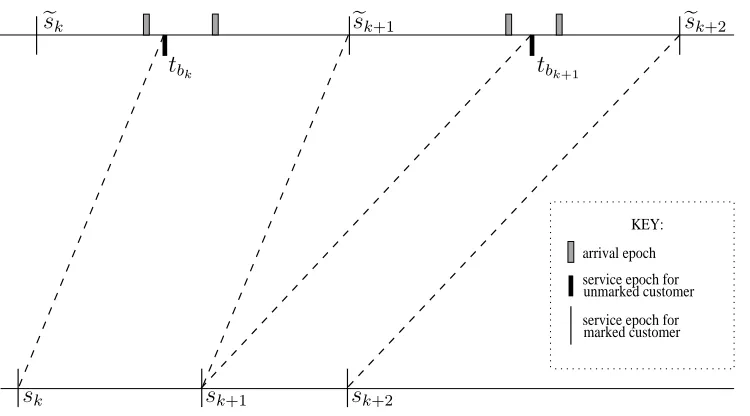
unmarked customer service epoch for arrival epoch
marked customer service epoch for
KEY:
sk sk+1 sk+2
e
sk esk+1 esk+2
[image:17.595.87.462.373.581.2]tbk tbk+1
Figure 2: Possible realizations ofQ(bottom) and Qe(top) under Coupling 2. The dia-gram shows the time horizons near thek-th service transitions of the marked customer in the two processes. The service epochs for whichCebecomes level withC after the
k-th and(k+ 1)-th services ofCe are given bytbk andtbk+1, respectively. The arrival
Theorem 2
Consider an M/M/1 Bernoulli feedback system and let π ∈ S∞ be any symmetric population joining policy. Then, for eachx = 0,1,2, . . ., V(x+ 1, π)−V(x, π) ≥ (1−p)E(W).
Proof
Consider realizations of the two processesQ andQe under Coupling 2. Assume that there are initiallyxcustomers ahead ofCinQandx+ 1customers ahead ofCeinQe and that all customers in bothQandQeuse the decision rule inferred by the symmetric policyπ∈S∞.
Fork= 1, . . . , K, letPkdenote the proposition: Xe(esk)≥X(sk)andesk ≥sk.
Assume thatK >1and thatPk holds for somek∈ {1, . . . , K −1}.
Due to the coupling, the position ofC inQats+k is exactly the same as that ofCeinQe att+b and their relative positions stay the same over the respective intervals(sk, sk+1]
and(tb,esk+1]. The last service completion inQein the interval(tb,esk+1]occurs whenCe
completes its next service, soCcompletes its next service at the corresponding epoch andsk+1 =sk+tb+d−tb. At that point Cis either fed back in the same way as Ceif
k+ 1 < KorC departs likeCeifk+ 1 =K.
The arrival, service completion, and feedback processes, forQover the interval(sk, sk+
tb+d−tb]completely mirror those inQeover the interval(tb, tb+d]. However, the num-berXe(t+b )inQeatt+b is, by construction, at least as great asX(s+k)inQ. Furthermore, consider anyt ∈ (0, tb+d−tb). Then whileXe(tb +t) > X(sk+t), the actual queue size dependent joining decision inQmay differ from the corresponding decision inQe; however, if for somet∗ ∈(0, tb+d−tb)the queue sizes are the same (i.e.Xe(tb+t∗) =
X(sk +t∗)), then the joining decisions will be the same for all t ∈ [t∗, tb+d −tb), and hence the queue sizes will stay equal over the corresponding intervals inQandQe. Thus, by construction,Xe(esk+1) ≥ X(sk+1). Finally, by assumption,esk ≥ sk and by constructiontb ≥esk, so thatesk+1 =tb+d =tb+ (tb+d−tb)≥sk+ (tb+d−tb) = sk+1.
ThusPk+1 also holds.
By construction, Xe(es0) = Xe(0) = x+ 1 > x = X(0) = X(s0), C starts b = 1
customer ahead of Ce in their respective systems, and completes its first service at
s1 = es1 −t1 wheret1 is the service completion epoch of the first customer served in
e
Qafter s+0. Using a similar argument to the one in the preceding paragraph, it also follows that Xe(es1) ≥ X(s1). Thus P1 holds here (and in the case where K = 1).
Hence, and in particular,esK ≥sK.
ex-pected extra timeCespends inQein that case isE(W).
Now, for eachk, the memoryless property of the Exponential distribution implies that the valuera+1 −tb used in constructing the arrival epochs for the interval (sk, sk+1)
is again an independent observation from the same Exponential inter-arrival distribu-tion. Thus, when we take expectation over all possible realizations ofQe the coupling also generates an expectation over all possible realizations of Q with just the right distributions for the inter-arrival (and service) times. ThusV(x+ 1, π)−V(x, π) ≥
(1−p)E(W). ¤
4
Monotonicity and continuity in the threshold
g
In this section we again consider aGI/G/1Bernoulli feedback queueing system but now assume all customers use the same threshold joining rule[L, q]. Recall from sec-tion 2.2 that the rule can be written in compact form as[g], where g = L+q. We consider the dependence of the expected sojourn time on the joining rule and show that it is a continuous function of g, which is constant for g ∈ [0,1], and is strictly increasing forg ≥1.
To motivate the population joining rule, consider what would happen if, instead of join-ing the feedback queue, customers could join an alternative queuejoin-ing system where the expected sojourn time was fixed atθ. We assume customers always join the feedback system when it is empty on arrival. However, if the queue size on arrival is x ≥ 1, we assume that each arriving customer joins the feedback queue only if their expected sojourn time is less than the fixed sojourn time in the alternative queue. In this case, the results of the previous section mean that each customer will use a threshold joining rule. Our focus here is on the behaviour of the expected sojourn time of an individual customer that does join the feedback queue when all the other customers are using the same threshold joining rule[g].
Now let g = L+q and eg = Le +qedenote the threshold values for two threshold joining rules withg < eg, so that eitherL < LeorL= Le andq < qe. Let v(x, β,[g]∞) (resp. v(x, β,[eg]∞)) denote the sojourn time for a customer who joins when there are alreadyx≥1customers in the system, when all other customers are using joining rule [g](resp.[eg]) and the customer in service on joining has residual service timeβ. Let the expected value of v(x, β,[g]∞) (resp. v(x, β,[eg]∞)) be denoted by V(x, β,[g]∞) (resp.V(x, β,[eg]∞)).
use[eg]. We then show that this second possibility happens on a set of positive proba-bility, so thatV(x, β,[eg]∞)> V(x, β,[g]∞).
Assume that there are initially x customers ahead of both C in Q and Ce in Qe. As-sume also that all other customers inQuse the same threshold joining policyπ= [g]∞ and all other customers inQe use the same threshold joining policyπ = [eg]∞, where
e
g > g.
Lemma 4.1 Consider realizations of the two processes Q and Qe under Coupling 1 with y = x. Let τ denote the set of epochs at which C or Ce (or both) complete a service and neither have yet departed, and let s and t denote successive epochs in
τ∪ {0}. Then
(i) the positions ofCandCerelative to each other do not change in(s, t) (ii) ifXe(s+)≥X(s+)thenXe(t)≥X(t)
(iii) ifX(s+) = Xe(s+) + 1thenX(t)≤Xe(t) + 1.
Proof
The argument is exactly the same as that for Lemma 3.1, except for the part relating to the changes in the respective queue sizes at arrival epochs.
Under the given policies a customer arriving inQatzwhen the queue size isxjoins if and only if eitherx < Lorx =LandU ≤ q, and a customer arriving inQeatzwhen the queue size isxjoins if and only if eitherx <Leorx=LeandU ≤ eq, where either
L <Le, orL=Leandq <qe.
If X(z) < Xe(z), then X(z+) ≤ Xe(z+), whatever the respective joining decisions. IfX(z) = Xe(z), then the customer will join inQif and only if either X(z) < Lor
X(z) = LandU ≤ q. SinceX(z) = Xe(z)and eitherL < Le orL = Leandq < qe, the customer joining inQimplies either Xe(z) < Le orXe(z) = Le andU ≤ eq, so the customer must also join inQe. Thus, at each arrival epoch in (s+, t), X(z) ≤ Xe(z) impliesX(z+)≤Xe(z+), giving (ii).
Similarly, ifX(z) = Xe(z) + 1, then the customer will join inQonly if the customer in
e
Qalso joins, so the customers either join in both queues (givingX(z+) = Xe(z+) + 1), neither queue, or just inQe (giving X(z+) = Xe(z+)). Combined with the argument
used to establish (ii), this gives (iii). ¤
Lemma 4.2 Consider realizations of the two processes Q and Qe under Coupling 1 with y = x. Let K denote the common number of visits both C and Ce make to the server in each realization, and let s1, . . . , sK and es1, . . . ,esK denote the service completion epochs forC andCerespectively. Then Xe(sk) ≥ X(sk)andesk ≥ sk for
Proof
Fork= 1, . . . , K, letPkdenote the proposition: Xe(sk)≥X(sk)andesk ≥sk.
First assumeK = 1. At t = 0, C andCe are level withx customers ahead of them. From Lemma 4.1, these relative positions are maintained untilCcompletes service, so
s1 =es1. Moreover,Xe(0+) = X(0+)so again from Lemma 4.1 (ii),Xe(s1)≥ X(s1).
ThusP1 is true.
The proof for the case K > 1 follows in exactly the same way as in Lemma 3.2,
except that we invoke Lemma 4.1 instead of Lemma 3.1. ¤
Theorem 3 Consider aGI/G/1Bernoulli feedback system and let[g]∞and[eg]∞be symmetric threshold population joining policies with0≤g <egandeg ∈[0, B). (i) Suppose eg ≤ 1. Then V(0,[eg]∞) = V(0,[g]∞), and for each x = 1,2, . . . and
β >0,V(x, β,[eg]∞) =V(x, β,[g]∞).
(ii) Supposeg ≥1. Then there existsδ0 >0such thatV(0,[eg]∞)−V(0,[g]∞)≥ δ0,
and for each x = 1,2, . . . and β > 0, there exists δx > 0such that V(x, β,[eg]∞)−
V(x, β,[g]∞)≥δ x.
Proof
Consider realizations of the two processesQ andQe under Coupling 1. Assume that there are initiallyxcustomers ahead of bothCinQandCe inQe. Assume also that all other customers inQare using the same threshold population joining policyπ= [g]∞ and all other customers inQe are using the same threshold joining policy π = [eg]∞, whereeg > g.
First suppose that0 ≤ g < eg ≤ 1. The sojourn times of the marked customers in the two processes will differ only if there is a disparity in the queue lengths during their stay in the systems. A customer is admitted into the queue of either process only if the queue is empty just prior to arrival. Clearly, however, the marked customer will have left by then, thus establishing (i).
Let s1 be as defined in Lemma 4.2. Now suppose that 1 ≤ g < eg, and let Rx de-note the set of realizations for which X(s1) = L and Xe(s1) = L + 1. If L < Le,
thenRxwould include for example realizations in which no customers arrived during the service periods of the firstxcustomers, all thesex customers departed following service,Lcustomers arrived during the (first) service period forC(and henceCe), and
For realizations in Rx with K = 2, C departs Q at s2 one service period ahead of
e
Cand the expected extra timeCespends inQein that case isE(W). From Lemma 4.2, in all other realizationsC completes all its services either level withCeor at least one service period ahead. Thus, taking expectation over all possible realizations, we have
V(x, β,[eg]∞)−V(x, β,[g]∞)≥p(1−p)P(R
x)E(W) = δx>0. ¤
We now introduce a third coupling which we will use to show that the expected sojourn timeV(x, β, π)is continuous ingfor symmetric threshold policies[g]∞. The coupling is designed to ensure that the queue length inQeis no less than that ofQ.
Coupling 3 SetS0 =Se0 =β,T =Te,W =Wf,U =Ue,F =Fe. ¤
Under Coupling 3, the successive arrival epochsAk andAek are the same in both sys-tems; the successive service completion epochsSk andSek are the same, at least until one or other system is empty; and the successive feedback variables are the same. However, although the successive joining variablesUk and Uek are the same, the suc-cessive arrival joining decisions will not necessarily be the same. Ck joins Q if and only ifUk ≤uk(X(Ak)), and similarly forCek. Thus the arrival joining decisions may differ in cases when the queue sizesX(Ak)andXe(Ak)differ, or when the queue sizes are the same but the actions specified by the decision rulesukandeukdiffer.
Now consider realizations of the processes in Qand Qe under Coupling 3, withg =
L+q andeg = L+qe, such that0 ≤ q < eq < 1, such thateg ∈ [0, B). This means that service and arrival events are identical under both processes, except that at queue length L an arriving customer inQe has a probability(qe−q)of being accepted when the corresponding customer is rejected inQ. The strategy will be to construct an upper bound onV(x, β,[ge]∞)−V(x, β,[g]∞)which can also be shown to tend to0aseg−g tends to0.
Theorem 4 Consider aGI/G/1Bernoulli feedback system and let[g]∞be a symmet-ric threshold population joining policy withg ∈[0, B). ThenV(0,[g]∞)is a continu-ous function ofg, and, for eachx= 1,2, . . .andβ >0,V(x, β,[g]∞)is a continuous function ofg.
Proof
(so s1 = es1, . . . , sk = esk) but complete their(k + 1)-st service at different epochs (sk+1 6= esk+1). Let E0 denote the remaining set of realizations for which C and Ce
complete all their services at the same epochs, soE0, E1, . . .form a partition of the set
of all possible realizations.
Because the two systems start in identical initial states and are coupled to have the same sequence of inter-arrival and service times, a realization inEk (k ≥ 1) occurs only ifCis fed back at leastk times,C andCehave exactly the same service comple-tion epochssr, r = 1, . . . , k, and there is at least one arrival in the period (sk−1, sk) who joins the system inQebut not inQ; i.e. this customer arrives when there areLin both systems and has a joining decision variableU withq < U ≤qe.
Let Ek1 denote the event that C is fed back at least k times and C and Ce have ex-actly the same firstk service completion epochs sr, r = 1, . . . , k. LetEk2 denote the event that there is at least one arrival in the period(sk−1, sk)who joins the system in
e
Qbut not inQ, and letDdenote the difference in the sojourn times ofCandCe. Then
Ek ⊂Ek1 ∩Ek2 soP(Ek)≤ P(Ek2|Ek1)P(Ek1)andE(D) =
P∞
k=1E(D|Ek)P(Ek)≤
P∞
k=1E(D|Ek)P(Ek2|Ek1)P(Ek1).
Given that Ek happens, any difference in the sojourn time is due only to the differ-ence between their sojourn times fromsk onwards. Since there can be at mostL+ 1 customers in each system, the expected time C spends in the system between each service completion epoch is at most(L+ 1)E(W)and the expected number of passes through the system aftersk is1/(1−p), so the expected sojourn time ofC fromsk onwards is no greater than(L+ 1)E(W)/(1−p). Arguing similarly forCe,E(D|Ek) is at most2(L+ 1)E(W)/(1−p).
Also,Ek1 occurs only ifCis fed back at leastk times, soP(Ek1)≤pk.
Finally, we derive a bound onP(Ek2|Ek1)as follows. Consider an arrival process that starts with an arrival at timet= 0. LetZdenote a random variable independent of the arrival process whose distribution is the same as that of the sum ofL+ 1independent service times, and let Y denote the number of arrivals in the closed interval [0, Z]. ClearlyY is almost surely finite (Feller 1966) soP∞r=0P(Y =r) = 1.
Now consider a realization in Ek1, so C and Ce are both fed back together to the end of their respective queues atsk−1 = esk−1 and have the samek-th service completion
epochsk = esk. Since the population joining rules are threshold rules with threshold values of the formg =L+qandeg = L+qe, the total number in each queue will be at mostL+ 1and so the timesk−sk−1until their next service completion will be no
num-ber of arrivals in[sk−1, sk]will be stochastically smaller than the number of arrivals in the interval[0, sk−sk−1]for an arrival process that starts with an arrival att = 0, and
this will in turn be stochastically no greater thanY. Thus if M denotes the number of arrivals to (both)Q and Qe in [sk−1, sk], thenM is stochastically smaller than Y. Since[1−(qe−q)]Y is strictly decreasing in Y (by noting that [1−(qe−q)] < 1),
E([1−(qe−q)]M)≥E([1−(eq−q)]Y).
LetU1, U2, . . . be a sequence of independent random variables each with a Uniform
distribution on(0,1]. Think ofUr as the joining variable of ther-th arrival aftersk−1.
Now givenEk1 occurs, Ek2 fails to occur if all joining decisions are the same in both systems in the interval [sk−1, sk], which will follow if Ur does not lie in the interval (q,eq]for ther-th arrival in the interval,r≥1, sinceX(s+k−1) = Xe(es+k−1). Thus, using the fact that theUr are independent of all other variables, we have that for a given q andqe,
1−P(Ek2|Ek1) ≥ P(M = 0) + ∞
X
r=1
P(M =r,
r
\
j=1
{Uj ∈/ (q,eq]})
= P(M = 0) + ∞
X
r=1
P(M =r)P( r
\
j=1
{Uj ∈/ (q,qe]})
= P(M = 0) + ∞
X
r=1
{1−(qe−q)}rP(M =r)
= ∞
X
r=0
(1−(qe−q))rP(M =r)
= ∞
X
r=0
(1−(eg−g))rP(M =r)
= E[(1−(eg−g))M].
It follows thatP(Ek2|Ek1)≤1−E[(1−(eg−g))M]≤1−E[(1−(eg−g))Y]. However, |(1−(eg −g))Y| ≤ 1and (1−(eg −g))Y −→ 1as eg−g → 0almost surely (using the fact thatY is almost surely finite). Hence, by the dominated convergence theorem,
E[(1−(eg−g))Y]−→1aseg−g −→0, and thusP(E2
k|Ek1)−→0also. Thus
E(D) = ∞
X
k=1
E(D|Ek)P(Ek)
≤ ∞
X
k=1
E(D|Ek)P(Ek2|Ek1)P(Ek1)
≤ [1−E([1−(eg−g)]Y)][2(L+ 1)E(W)/(1−p)] ∞
X
k=1
pk
¤
5
Individual Nash equilibrium and social optimality
So far, we have looked at joining decisions for an isolated Bernoulli feedback queue. We now assume that the cost of balking upon arrival to Qis some constant value θ. We can think of θ as the time spent (or, alternatively, the cost of) using a ’private’ or self-service system which is slower than Q, in the sense thatθ is greater than the total expected time spent at the server for each customer inQ. More precisely, it will be assumed that 1/µ(1−p) < θ; this condition says that it is always optimal for a customer to joinQif there are no customers in the system upon arrival, and there will be no further customers joining the system in the future. The joining decision depends only on the observed number of customers atQon arrival. Customers who joinQare not permitted to renege during their sojourn, nor are those who balk permitted to join
Qat a later stage.
We consider first what happens when customers make their own individual joining decisions and each customer is only interested in minimizing their own expected so-journ time, or cost. Due to the Bernoulli feedback characteristic, the soso-journ time of a particular customer inQmay be affected by the number of customers in the queue during its sojourn, which in turn is affected by the decisions of subsequent arriving customers. This problem fits into a game theoretic framework. We derive the Nash equilibrium solution for the state dependent stationary game that arises and show that under this regime, the joining rule for each customer has a particular (possibly ran-domized) threshold form.
We then consider what happens when the joining decision for each customer is made by a central controller or social optimizer, whose goal is to minimize the overall ex-pected cost per customer, averaged across customers admitted toQand those that balk. In this case we show that there is a deterministic threshold rule which characterizes a socially optimal joining rule.