ORIGINAL RESEARCH ARTICLE
SPATIAL CHARACTERIZATION AND INTERPOLATION OF PRECIPITATION DATA
*1
Eric Asa,
2Joseph F.J. Membah and
2Edmund Baffoe-Twum
1
North Dakota State University, Department of Construction Management and Engineering, Dept. 2475,
Box 6050, Fargo, ND, 58108-6050. Fargo, ND, USA
2
North Dakota State University, Department of Civil and Environmental Engineering, Dept. 2470,
Box 6050, Fargo, ND, 58108-6050.
Fargo, ND, USA
ARTICLE INFO ABSTRACT
Being able to accurately predict point or a real precipitation data at unsampled locations or areas using measured precipitation data is important in the work of agriculturists, hydrologists, climatologists, engineers, and others. Precipitation phenomenon is a complicated process due to the spatial variability, uncertainty, and complexity of the meteorological processes underlying its formation. There is a need to investigate the use of the most common geostatistical techniques to characterize, interpolate, and analyze precipitation data with the intent to identify the best set of semivariogram and spatial interpolation algorithms for characterizing precipitation data in a region of interest. Linear kriging (ordinary kriging, simple kriging, and universal kriging) and nonlinear kriging (indicator kriging, probability kriging, and disjunctive kriging) algorithms were used in this research project to characterize and interpolate precipitation data. Gaussian, circular, spherical and exponential semivariograms were employed with the six interpolation algorithms to characterize the precipitation data. Statistical measures of correctness (mean prediction error, root-mean-square error, standardized root-mean-square error, average standard error) from cross-validation were used to compare the combination of kriging and semivariogram algorithms. The most accurate results were obtained by using indicator kriging (IK) with a circular semivariogram for spatial characterization and interpolation of the precipitation data. IK and circular variogram algorithms were used to perform multi-scale analysis of the wet and dry months.
Copyright © 2019,Eric Asa, Joseph F.J. Membah and Edmund Baffoe-Twum. This is an open access article distributed under the Creative Commons Attribution License, which permits unrestricted use, distribution, and reproduction in any medium, provided the original work is properly cited.
INTRODUCTION
Precipitation (rainfall and snow) data obtained from radar, or measured at structured weather stations several miles apart are used to estimate data values at a point or within a specific area. The estimates derived from its analysis are critical inputs into hydrological, ecological, flood prediction/protection, and other models (Running et al. 1987; Dolph et al. 1992; Daly et al. 1994; Goovaerts, 2000). Accurate estimates of precipitation data are required for many applications in hydrologic engineering, environmental science, and other disciplines. A
fundamental problem in hydrology is the spatial
characterization and estimation (interpolation) of precipitation values at unsampled locations using the surrounding measured) precipitation data.
*Corresponding author: Eric Asa,
North Dakota State University, Department of Construction Management and Engineering, Dept. 2475, Box 6050, Fargo, ND, 58108-6050. Fargo, ND, USA
An accurate estimation of precipitation data values could be achieved through the deployment of a densely populated network of instrumentation (and personnel) to collect and record the data. This costly process could be avoided by employing stochastic characterization, which uses neighboring precipitation data points to estimate the precipitation values at unsampled locations and specific areas of interest (Jones and Thornton, 1997; Wilks, 1999; Goovaerts, 2000). Even though stochastic characterization has been employed in hydrology and engineering studies, it is not evident from the literature which method is the most suitable for characterizing
precipitation data. Various kriging techniques and
semivariograms were developed but there has been limited interest in exploring their merits and demerits or comparison of the algorithms to each other. Thus, there is a need to use geostatistical techniques to characterize, interpolate and analyze precipitation data with the intent to identify and compare the most accurate set of semivariogram and spatial
ISSN: 2230-9926
International Journal of Development Research
Vol. 09, Issue, 02, pp.25863-25877, February, 2019
Article History:
Received 19th November, 2018 Received in revised form 26th December, 2018 Accepted 13th January, 2019 Published online 28th February, 2019
Available online at http://www.journalijdr.com
Key Words:
Kriging, Cross-validation, Semivariogram, Precipitation.
Citation: Eric Asa, Joseph F.J. Membah and Edmund Baffoe-Twum. 2019. “Spatial characterization and interpolation of precipitation data”, International Journal of Development Research, 09, (02), 25863-25877.
interpolation algorithms for characterizing precipitation data in a region of interest. The best method for making comparisons is to employ cross-validation techniques to compare the predicted and actual (observed) precipitation data for each set of semivariogram and kriging techniques. The predominant methods that have been employed to estimate climate data values are inverse distance/distance weighting, Thiessen polygon/interpolating polynomials, principal component analysis, regression, kriging, neural networks, genetic algorithms, splines, and Markov models (Thiessen, 1911; Delhomme, 1978; Stewart and Cadou, 1981; Stern and Coe, 1984; Tabios and Salas, 1985; Bedient and Huber, 1992;
Phillips et al. 1992; Abtew et al 1993; Bardosy, 1993;
Eischeid et al. 1995; Hulme at al. 1995; Lennon and Turner, 1995; Hammond and Yarie 1996; Holdaway 1996;
Martinez-Cob 1996; Ashraf et al. 1997; Dobson and Marks 1997; Jones
and Thornton, 1997; Demyanov et al. 1998; Huang, et al.
1998; Hutchinson, 1998; Hutchinson and Gessler, 1994; Nalder and Wein, 1998; Wilks 1999; Goovaerts, 2000). Entekhabi et al. 1999 and Kyriakidis et al. 2004, emphasizes the importance of research in hydrology and engineering to accurately characterize and interpolate precipitation values. Limited area models have been used to improve the accuracy of regional-scale of precipitation data analysis (Giorgi and Mearns, 1991; Kim and Soong, 1996; Miller and Kim, 1996; Kim et al. 1998). A computationally expensive dynamic downscaling procedure has been used.
The area with the most uncertainty in hydrologic models employed in operational river stage forecasting is the quantitative precipitation forecast (Krzysztofowicz, 1998; Seo
et al. 2000). Geostatistics offers the best approach to characterize and interpolate precipitation data but most of the studies have been limited to only one or two algorithms with little justification for the choice of algorithms (Bras and Rodriguez-Iturbe, 1985; Seo et al. 2000; Kyriakidis et al. 2001; Kyriakidis et al. 2004). Past research indicates that the assumption of spatial correlation and regionalization in hydrological studies are justified even with moderate deviations, because regional analysis still yields more accurate quantile estimates than at-site analysis (Lettenmaier and Potter,
1985; Lettenmaier et al. 1987; Hosking and Willis 1988; Potter
and Lettenmaier, 1990; Kyriakidis et al. 2004; Gonzales and Valdes, 2008). Thus, geostatistics is an acceptable methodology for the characterization and interpolation of precipitation data (Delhomme 1978; Creutin and Obled, 1982; Lebel et al. 1987; Azimi-Zonooz et al. 1989; Barancourt et al. 1992; Bacchi and Kottegoda 1995; Goovaerts, 2000, Germann and Joss, 2001; Bernes et al. 2004; Bernes, et al., 2009). In past research, kriging methods such as ordinary kriging, kriging with a trend, universal kriging and others have been used to incorporate the heterogeneity and spatial correlation of climate variables into the estimation of climate data values
(Delhomme, 1978; Tabios and Salas, 1985; Phillips et al.
1992; Bardosy, 1993; Hammond and Yarie, 1996; Holdaway,
1996; Martinez-Cob, 1996; Ashraf et al. 1997; Nalder and
Wein, 1998; Goovaerts, 2000; Llyod, 2005; Bargaoui and Chebbi, 2009).
Kriging is a generalized least-square, spatial
estimation/interpolation method that was introduced by Krige (1951) and formalized (developed into a mathematical model) by Matheron (1963). Kriging is an optimal (best linear unbiased) spatial interpolation or prediction procedure based on using regression analysis against observed data points
obtained from surrounding locations. It is weighted against spatial covariance values and optimized with respect to specific error criteria (Bohling, 2005). Kriging could be described as a methodology that employs the notion of regionalized variables or autocorrelation to estimate values at unsampled locations. It is a linear regression technique that minimizes the estimation from fitted covariance models or
semivariograms (Royle et al. 1981; Lam 1983; Heine 1986;
Davis 2002). Kriging is used to construct a minimum error variance linear estimate at a location where the actual value is unknown. It could be employed to estimate a series of posterior conditional probability distributions from which unsmoothed images of the attribute spatial distribution are drawn (Deustch and Journel, 1998). Kriging could be used as a tool for interpolating precipitation data, calculating the conditional cumulative distribution function (ccdf) values and as a mapping algorithm (Goldberger 1968; Luenberger, 1969; Matheron, 1971; David 1977; Brooker 1979; Hohn, 1988; Journel, 1989; Isaaks and Srivastava 1989; Cressie 1991; Goovaerts 1997; Deustch and Journel, 1998; Chiles and Delfiner, 1999; Goovaerts, 2000; Lloyd and Atkinson, 2001; Journel and Huijbregts, 2003). Stochastic characterization and interpolation tools (geostatistics) are a collection of numerical techniques that could be used to analyze spatially distributed data and aid in decision making. Even though many precipitation research studies have acknowledged the need for spatial modeling approaches, there is limited evidence of research approaches aimed at defining optimal spatial
interpolation methods (Goodrich et al. 1995; Guan et al.
2005). The predominant practice is using a single kriging method together with one semivariogram model to characterize and interpolate climate data (Delhomme, 1978; Tabios and Salas, 1985; Phillips et al., 1992; Bardosy, 1993; Hammond and Yarie, 1996; Holdaway, 1996; Martinez-Cob, 1996; Ashraf et al. 1997; Atkinson and Llyod, 1998; Nalder and Wein, 1998; Goovaerts, 2000; Llyod, 2005).
According to the work of Nalder and Wein (1998), four semivariogram models were used for each variable (temperature and precipitation) each month, leading to a total of 120 models. None of the semivariogram models were identified and accorded the same attention as the interpolation algorithms. There was no attempt to find the combination of kriging and semivariogram algorithms most suitable for characterizing and interpolating the climate data. A fundamental requirement in geostatistics is that the model developed should represent the structure of the unknown function to be estimated. Therefore, models developed using geostatistic methods must be checked and validated (Box and Jenkins, 1976; Delfiner, 1976; Dubrule, 1984; Kitanidis and Vomvoris, 1983; Davis 1987; Borgman, 1988; Kitanidis, 1988; Snodgrass and Kitanidis, 1997). There is little evidence about how the data affects the performance of the kriging technique and the semivariogram models. It is speculated that it may not be possible to find the best kriging technique and semivariogram for a given precipitation data set (Burrough and
McDonnell, 1998; Jones et al., 2003; Zhou et al. 2007).
MATERIALS AND METHODS
of the state of North Dakota. The six spatial interpolation techniques and the four semivariogram models are the most widely-used geostatistical algorithms and are employed by the majority of researchers in geostatistics. At the genesis of the research, exploratory data analysis techniques were used to determine the linear statistical properties of the data. If the data were lognormally distributed, it would have been transformed prior to semivariogram modeling and kriging. The combination of six kriging methods and four semivariogram models were sequentially applied to the precipitation data. There was no scientific basis for the order of application of the methods. The actual ordering was done randomly. Thus, there were no prejudicial effects for the ordering of the kriging and semivariogram algorithms. Each kriging run was followed by cross-validation and the necessary statistics were compiled, analyzed, and compared. The best set of kriging and variogram algorithms were then used to study the seasonal differences and multi-scale effects of the wet and dry months. Figure 1 summarizes the research methodology.
Figure 1. Summary of Research Methodology
Precipitation Data
The precipitation data used in this study was extracted from the National Climate Data Center (NCDC) Summary entitled Climatography of the United States No. 81 (NOAA, 2009). The extracted data contains monthly precipitation (for each recording station) data points for a thirty-year period termed normals (for the period 1971-2000). The extracted data was for the state of North Dakota. Figure 2 provides the location of the weather stations where the data was recorded in North Dakota.
Figure 2. Map of North Dakota Showing the Location of the Weather Stations
Methods
Mathematical Modeling of Spatial Structure: A semivariogram model (a relationship between meteorological distance and Euclidean distance) is an important statistical tool
used to measure spatial correlation in all geostatistical applications (Cressie, 1985; Goovaerts, 1997; Chiles and Delfiner, 1999; Deutsch, 2002; Journel and Huijbregts, 2003;
Menezes et al. 2005). The semivariogram quantifies the spatial
variability of the variables by computing the variance of the variables measured at some distance h, apart. Thus, the semivariogram is an important tool in the analysis of spatial continuity of the natural phenomena under investigation. Often, as the separation distance increases, the samples become more dissimilar and hence the semivariogram/variance increases. In order to have one and only one solution to the kriging equation, the left-hand covariance matrix must satisfy a mathematical condition termed positive definiteness. During geostatistical characterization of a regionalized variable/ phenomenon, an estimated semivariogram is needed for kriging/interpolation (determining kriging weights) of the random fields with similar spatial properties, understanding the spatial structure of the variable, optimal sampling design and exploring the scaling properties of the models using the variable as an input (Matheron, 1962; Burgess and Webster,
1980; McBratney et al.1981; Papritz and Webster, 1995;
Genton, 1998; Oliver, 1999; Lark, 2000; Deutsch, 2002). Thus, the semivariogram is used to simulate the observed variability present in the available data (Gringarten and Deutsch, 2001).
The positive definite condition could be satisfied by ensuring that the functions combined to form the semivariogram model are known and tested to be positive definite. Therefore, a linear combination of such functions is positive definite (additivity of positive definiteness). The basic models of regionalization (semivariogram) are pure nugget effect - white noise (Journel and Huijbregts, 2003), spherical (Deutsch and Journel, 1998), Gaussian (Goovaerts, 1997), hole effect - cardinal sine, triangle, cubic, circular (Chiles and Delfiner, 1999), generalized Cauchy (Journel and Huijbregts, 2003), Bessel, power-law, logarithmic - de Wijsian (Chiles and Delfiner, 1999) and other models. Besides the power model, all of the other semivariogram models are termed bounded, that is they reach a constant sill at some distance, termed the range. The most commonly used semivariograms are the spherical, circular, exponential, and Gaussian models. Generally, experimental semivariogram models are built as a linear combination of two or more types of basic models. The fundamental elements of the modeling process are (1) calculating an experimental semivariogram; (2) considering meteorological information and knowledge of the area (if available) to supplement the calculated points; and (3) fitting a licit positive definite model to the data. The resulting semivariogram model must capture all the major features of the phenomenon (precipitation data) under investigation.
For two sample values z(x) and z(x+h) at two points x and x+h separated by the vector h, the semivariogram obtained by using Matheron’s method of moments (Matheron, 1962) could be defined as the expected value (equation 1);
(1)2 h E Z x Z xh 2
Where 2γ is the semivariogram and γ(h) is the semivariogram.
[image:3.595.38.286.547.705.2]Goovaerts 1998; Chiles and Delfiner 1999; Lark 2000; Journel and Huijbregts 2003):
, , (2) 2 1 ) ( 2 1 2 ) ( 2 A h x x h x Z x Z E h x Z x Z h N h h N
The linear models of regionalization that would be employed in this research are the circular, spherical, exponential, and Gaussian semivariograms. These are presented in Table 1. In the Gaussian model, the range is given by 1.732a and the sill is reached asymptotically. For small distances, a local variation could be interpreted as a stationary Gaussian structure or as a drift effect (Chiles and Delfiner, 1999; Journel and Huijbregts, 2003). The exponential semivariogram reaches its sill asymptotically, as h turns to infinity. The practical range (95% of the sill or a correlation of only 5%) of the semivariogram is about 3a. The gradient of the spherical and exponential models are the same at h = 0. The gradient of the Gaussian model is zero at h = 0.
Mathematical Modeling of Spatial Interpolation (Linear and Non-linear) Algorithms: Both linear (ordinary kriging, simple kriging, and universal kriging) and nonlinear (indicator kriging, probability kriging, and disjunctive kriging)
interpolation techniques were used in this study. The basic
assumptions made in the kriging estimator were: the unknown
sample data, z(x) and the n sample values belong tothe
regionalized variables, Z(x), and Z(x1),.... , Z(xn). There were
no measurement or positional errors. For any two points x1 and
x2 in the area over which z(x) is being estimated, the
covariance Cov(Z(x1), Z(x2)) of the associated regionalized
variables Z(x1) and Z(x2) were known. The non-negative
matrix of covariances between the measured variables (data) at the sample points were positive definite. The covariance between x1 and x2 were shortened as (equation 3):
)) ( ), ( ( ) ,
(x1 x2 Cov Z x1 Z x2
C
(3)
The trend in the area of interest is homogeneous. Thus, the mean of the regionalized variables is the same for the data points xn in the area in which z(x) is being estimated. If a trend
exists in the area of interest, the stationarity of the local mean is relaxed and a non-stationary random function is employed to represent the mean (kriging with a trend or universal kriging). Kriging techniques are extensions or transformations of the generalized linear regression algorithm. The objective of kriging algorithms is to minimize the estimation or error variance σ2E, under estimator unbiasedness constraints (see
equation 4). That is:
s.t.
02 x Z x Z E x Z x Z Var x
Min E
(4)
[image:4.595.170.430.402.556.2]Linear kriging algorithms are distribution-free, linear interpolation techniques, which are akin to linear regression.
Table 1. Four Commonly Used Variogram Models
Model Mathematical Representation Spherical Variogram otherwise c a h if 5 . 0 a h 1.5 c ) ( 3 a h h Circular
Variogram () 2 1 2arcsin 0 h a or 1 2
a h a
h a
h a h
h
Gaussian
Variogram ( ) 1 exp 32 0
2 h a h h Exponential
Variogram ( ) 1 exp 3 0 h a h h
Where c= sill; h = lag distance and a = range (Chiles and Delfiner, 1999, Deutsch and Journel, 1998, Goovaerts, 1998, Journel and Huijbregts, 2003).
Table 1. Linear and Nonlinear Spatial Interpolation Algorithms
Type Mathematical Representation
Linear Spatial Interpolation Algorithms Ordinary Kriging
. ( ) 1
( )1 1 * x m x x Z x x Z n i i i n i i OK
Journel and Deustch, 1998.
Simple Kriging . ( ) 1
1 1
* x x Z x x m
Z n x i i n i i SK
Journel and Deustch, 1998. Universal Kriging ( ) ( ). ( )
1 * i n i i KT x x Z x
Z
Goovaerts, 1997; Deutsch and Journel 1998; Chiles and Delfiner, 1999; Lloyd and Atkinson, 2001; Journel and Huijbregts, 2003.
Nonlinear Spatial Interpolation Algorithms Indicator Kriging
;
; |(n)
Prob
|( )
* * * n z x Z z x I E z x
i k k k
Journel, 1983 and 1986; Isaaks and Srivastava, 1989; Ying, 2000.
Probability Kriging
(; )
( ) (; ).
; ( )
(; ).
0.5
1 1
xz Ix z Fz xz px z F z x I k n k k k n k PK k
Disjunctive Kriging ( ) ( ( ))
1 * i n i i DK x Z x
Z
Matheron, 1963 and 1971; Rivoirard 1994; Journel and Huijbregts, 2003; Lark and Ferguson, 2004; Webster and Oliver, 2007.
[image:4.595.39.547.592.812.2]The linear kriging equations are depicted in the upper part of Table 2, where Z(x) is the random variable at the location x, all xi values are the n data locations, m(x)=E{Z(x)} is the
location-dependent expected value of the RV Z(x), ωi(x) are
the weights, and m is the constant mean. The ordinary kriging technique is a nonstationary algorithm, which involves estimating the mean value at each location, and it is generally applied in moving search neighborhoods. However, the covariance function is stationary. A location-dependent estimate of the mean is used to replace the constant mean of the simple kriging technique. In ordinary and simple kriging, the mean value of the variable is assumed to be constant (local stationarity) over the search area. In some practical situations the local mean varies over the search area. Kriging with a trend (universal kriging) involves situations where the local mean is variable over the study area. Kriging with a trend is meant to accommodate a non-stationary mean; where the expected value of Z(x) is a deterministic function of the coordinates. The random function, Z(x), is a combination of a trend component with a deterministic variation, m(x), and a residual component (with randomness or stochastic variation), R(x), as depicted in equation 11 in Table 2 (Goovaerts, 1997; Deutsch and Journel, 1998; Chiles and Delfiner, 1999; Lloyd and Atkinson, 2001; Journel and Huijbregts, 2003). In universal kriging, the residual component, R(x) is considered a stationary random variable with zero mean and a covariance, CR(h). A first degree polynomial (which avoids unpredictable
behavior at the outer margins of the data set) is used to set the trend.
The three nonlinear kriging algorithms used in this work were indicator kriging, probability kriging and disjunctive kriging. In this study, indicator kriging, probability kriging and disjunctive kriging algorithms, were used. Nonlinear kriging algorithms are linear kriging algorithms applied to nonlinear transformations of the data points into a continuous (Gaussian) variable (Journel and Deustch, 1998). Indicator kriging, which is a least-squares estimator of the cumulative distribution
function at a threshold or cutoff (zk), was introduced to update
prior probabilities into posterior or conditional probability distributions and was later extended to include inequality constraints (Journel, 1983 and 1986). Indicator kriging employs the samples in a neighborhood to estimate the probability of data points in a given area exceeding a defined threshold (Isaaks and Srivastava, 1989; Ying, 2000). In the application of indicator kriging, data are transformed into indicator values (0 and 1). Values that exceed a certain threshold are coded 1 and those below it are coded 0. The major advantage of indicator kriging is that different types of soft secondary data could be combined with direct data points and inequalities to estimate the quantity of interest. Probability kriging, a conditional cumulative distribution function model for Z(x), is a form of cokriging that uses the original values instead of their indicator transformations of the data values at thresholds different from that being estimated (Sullivan, 1984; Verly and Sullivan, 1985). In probability kriging, ωα and να are
the cokriging weights of the indicator data and the uniform data respectively. The weights are location (x) and threshold (zk) dependent; while p(xα) = F(z(xα)) Є [0,1] is the uniform
(cumulative distribution function) of the datum value z(xα). If
the stationary mean or the expected value is 0.5; then F(z) = Prob{Z(x)≤z} which is the stationary cumulative distribution function of Z(x). The estimates resulting from indicator and probability kriging are probabilities that the sample points in question are above the cutoff or the percentage of samples
above the cutoff. These probabilities could be used to estimate the actual values at the unsampled locations.
Disjunctive Kriging is a non-linear kriging method, which was introduced by Matheron (1963). It uses a bivariate probability model for the estimation of any function z(x). The disjunctive kriging technique is more accurate than the linear kriging methods but less accurate than the unknown conditional expectation of the variable. It is considered as an intermediate estimator (Journel and Huijbregts, 2003). In disjunctive kriging, the data points are assumed to be realizations of a second-order stationary bivariate diffusion process (Lark and Ferguson, 2004). In the disjunctive kriging estimator, λi are
non-linear functions of the data. Generally the expansion is truncated at p≤100. The most common form of the disjunctive kriging technique is the Gaussian diffusion process and Hermite polynomials could be used to transform the data into normality (Rivoirard, 1994; Lark and Ferguson, 2004; Webster and Oliver, 1992; 2007). Each experiment (semivariogram fitting and kriging run) was followed by cross-validation and the statistics were compiled, analyzed and compared. The mean prediction error (mean), the standardized mean prediction error (SM), the root-mean-squared prediction error (RMSE), the standardized root-mean-squared prediction error (RMSES), and the average standard error (ASE) were used to compare the characterization and interpolation results.
Model Checking and Statistical Comparison
Selection of the correct model is important to the success of all spatial interpolation and simulation studies. According to Irobi et al (2004), a correct model could be considered as the closest representation of a system because of the abstract complexity of natural processes. Cross-validation is the preferred model checking method (Stone, 1974; Bowman, 1984; Hardle and Marron, 1985). The complexity of meteorological processes, problems with sampling, and lack of knowledge, result in model uncertainty and cross-validation is used to check the accuracy and consistency of the interpolation techniques and algorithms (Voltz and Webster, 1990; Gotway and Rutherford, 1994; Deutsch, 1997; Chiles and Delfiner, 1999; Deutsch, 2002; Robinson and Metternicht, 2006). Cross-validation could be used choose between and/or compare weighting procedures, search strategies, and interpolation and simulation algorithms (Goovaerts, 1997; Chiles and Delfiner, 1999; Deutsch, 2002; Robinson and Metternicht, 2006; Emery and Ortiz, 2007). Cross-validation is used to evaluate the predictive capabilities of models (Stone, 1974).
In cross validation, the data is used to develop the model. In leave-one-out cross-validation, the entire set of available data is used to develop the model. When one data point is removed, the kriging model with the variogram is used to predict the missing data (Goovaerts, 1997; Deutsch, 2002; and Chiles and Delfiner, 1999). The actual and interpolated values are then compared. Equation 5 is used to assess the systematic error.
1 (Mean) Error Prediction Mean
1
*
n
i
i
i z x
x z n
(5)
Equation 6 represents the standardized mean prediction error:
n
i
x
iMean
n
SM
1
2
(6)
1
Equations 7 and 8 represent the root mean square prediction error and the standardized root-mean-square prediction error respectively.
1
RMSE
2 1 *
n i ii
z
x
x
z
n
1
RMSES
2 1 2
ni
x
iMean
n
ASE, the average standard error (ASE) is given by equation 9;
n
s
ASE
ASE also termed the standard error of the mean is the measure of the accuracy of the average of the prediction standard errors. The ASE has the property of increasing as the variability of the data increases, and decreasing as the sample size increases. In equations 5, 6, 7, 8 and 9, σ
variance at location xi; s is the standard deviation; n is the
number of data points. The statistics from equations 5, 6, 7, 8 and 9 are compiled and employed to assess and compare the models.
Statistical Decision Criteria and Optimality
The five statistics from equations 5, 6, 7, 8, and 9 were
evaluate the output of the combinations of six kriging and four semivariogram algorithms. The statistics of the best set of semivariogram and kriging methods were the following: (1) a small average standard error (ASE); (2) a mean prediction error (mean) near 0; (3) a standardized mean prediction error (SM) near 0; (4) a standardized root-mean-squared prediction error (RMSES) near 1; and (5) a small root
prediction error (RMSE) (Pardo-Igusquiza, 1998; Robinson and Metternicht, 2006). The root-mean-squared error of the preferred combination of kriging and semivariogram model is approximately equivalent (closest) to the average error. Using the equivalency of the root-mean-squared error (RMSE) and the average standard error (ASE) as the optimality criteria, the decision criterion is represented by the equation 10:
0
RMSE
ASE
For a number of n equiprobable models the decision rule is given by equation 11
)
(
ASE
RMSE
nMinimize
Multi-scale Spatial Analysis of Wet and Dry Months
Suppose a smaller random rectangular block with value Y superimposed on and used to sample a larger block with value Y2, the expected value of Y1 is Y2 and it is given by E(Y
Y2 . However this property could be violated if the data is not
gridded and/or the trend in all directions is not the same. The cross-validation statistics and variogram properties of the blocks would also be compiled and compared.
25868 Eric Asa, Joseph F.J. Membah and Edmund Baffoe
Equations 7 and 8 represent the root mean square prediction square prediction error
(7)
(8)
ASE, the average standard error (ASE) is given by equation 9;
(9)
ASE also termed the standard error of the mean is the measure average of the prediction standard errors. The ASE has the property of increasing as the variability of the data increases, and decreasing as the sample size increases. In equations 5, 6, 7, 8 and 9, σ2 (xi) is the
d deviation; n is the number of data points. The statistics from equations 5, 6, 7, 8 and 9 are compiled and employed to assess and compare the
Statistical Decision Criteria and Optimality
The five statistics from equations 5, 6, 7, 8, and 9 were used to evaluate the output of the combinations of six kriging and four semivariogram algorithms. The statistics of the best set of semivariogram and kriging methods were the following: (1) a small average standard error (ASE); (2) a mean prediction (mean) near 0; (3) a standardized mean prediction error squared prediction error (RMSES) near 1; and (5) a small root-mean-squared Igusquiza, 1998; Robinson squared error of the preferred combination of kriging and semivariogram model is approximately equivalent (closest) to the average error. Using squared error (RMSE) and optimality criteria, the decision criterion is represented by the equation 10:
(10)
For a number of n equiprobable models the decision rule is
(11)
scale Spatial Analysis of Wet and Dry Months:
Suppose a smaller random rectangular block with value Y1 is
superimposed on and used to sample a larger block with value is given by E(Y1|Y2) =
. However this property could be violated if the data is not gridded and/or the trend in all directions is not the same. The validation statistics and variogram properties of the blocks would also be compiled and compared.
RESULTS
Implementation and Discussion of Results
The experiments were conducted using the Geostatistical Analysts module of ESRI’s ArcGIS software (versions 9.3 and 10.3) and Minitab 17. The order of performance of the
experiments were: exploratory data
transformation (if required); fitting of a licit semivariogram to the data; use of each of the six spatial interpolation algorithms and the fitted semivariogram to characterize the data in a GUI environment; cross validation of the results an compilation of the resulting statistics; and development of tables and graphs to analyze, compare and select the most appropriate models (Chiles and Delfiner, 1999; Deutsch, 2002). Some processes have been combined with others in the descriptions that follow.
Exploratory Data Analysis: The monthly precipitation data
was averaged to develop an annual profile for each weather location sampled. The monthly maximum, average and minimum annual precipitation were determined and averaged for the thirty-year period. The data was subjected to exploratory statistical data analysis to understand it. The techniques employed were measures of central tendency, histograms plots, and quantile
average precipitation for each month (
[image:6.595.36.284.103.200.2]the sampled 118 weather stations spread over the state of North Dakota is presented in Figure 3. A histogram of the precipitation data for North Dakota is presented in Figure 4. The precipitation data was divided into the distinct f seasons. On the basis of the distinct four seasons the data showed different results. Minitab was used to fit distributions to the histograms of the four seasons. Whereas spring and fall seasons are approximately normal, the winter and summer are skewed. The descriptive statistics of the four seasons are presented in Table 3. Precipitation in summer (with a mean of 7.997) and spring (with a mean of 4.465) are higher than winter (with a mean of 1.365) and fall (with a mean of 3.824).
Figure 3. Plot of Monthly Precipitation Data for January to December of the Sampled 118 Weather Stations
Test for normality was performed on the four seasons and the results are presented in Figure 5. The graphical plot of normal percent versus the four season data depart from the fitted line both extreme ends. The Ryan
indicates that, at α values greater than 0.020, there is evidence that the data does not follow a normal distribution for the spring season. For the other seasons, the αs are less than the 0.05 confidence interval. The p
greater than 0.05 confidence interval, and thus the null hypothesis was rejected.
Asa, Joseph F.J. Membah and Edmund Baffoe-Twum, Spatial characterization and interpolation of precipitation data
Implementation and Discussion of Results
The experiments were conducted using the Geostatistical Analysts module of ESRI’s ArcGIS software (versions 9.3 and 10.3) and Minitab 17. The order of performance of the
experiments were: exploratory data analysis and
transformation (if required); fitting of a licit semivariogram to the data; use of each of the six spatial interpolation algorithms and the fitted semivariogram to characterize the data in a GUI environment; cross validation of the results and the compilation of the resulting statistics; and development of tables and graphs to analyze, compare and select the most appropriate models (Chiles and Delfiner, 1999; Deutsch, 2002). Some processes have been combined with others in the
The monthly precipitation data was averaged to develop an annual profile for each weather location sampled. The monthly maximum, average and minimum annual precipitation were determined and averaged year period. The data was subjected to exploratory statistical data analysis to understand it. The techniques employed were measures of central tendency, histograms plots, and quantile-quantile (Q-Q) plots. The average precipitation for each month (January to December) of the sampled 118 weather stations spread over the state of North Dakota is presented in Figure 3. A histogram of the precipitation data for North Dakota is presented in Figure 4. The precipitation data was divided into the distinct four seasons. On the basis of the distinct four seasons the data showed different results. Minitab was used to fit distributions to the histograms of the four seasons. Whereas spring and fall seasons are approximately normal, the winter and summer are d. The descriptive statistics of the four seasons are presented in Table 3. Precipitation in summer (with a mean of 7.997) and spring (with a mean of 4.465) are higher than winter (with a mean of 1.365) and fall (with a mean of 3.824).
. Plot of Monthly Precipitation Data for January to December of the Sampled 118 Weather Stations-North Dakota
Test for normality was performed on the four seasons and the results are presented in Figure 5. The graphical plot of normal cent versus the four season data depart from the fitted line both extreme ends. The Ryan-Joiner (RJ) test’s p-value indicates that, at α values greater than 0.020, there is evidence that the data does not follow a normal distribution for the For the other seasons, the αs are less than the 0.05 confidence interval. The p-values for the four seasons are greater than 0.05 confidence interval, and thus the null
Table
[image:7.595.81.520.78.784.2] [image:7.595.74.532.429.786.2]Mean Winter 1.365 Spring 4.465 Summer 7.997 Fall 3.824
Figure
Figure
25869 International Journal of Development Research,
Table 2. Descriptive Statistics for Precipitation Data
Mean St. Dev Minimum Maximum Skewness Kurtosis 1.365 0.2769 0.770 2.010 0.40 -0.36 4.465 0.5683 3.370 6.190 0.66 0.43 7.997 0.9866 5.630 9.930 -0.17 -0.78 3.824 0.5915 2.510 5.210 0.29 -0.39
Figure 4. Histogram and Normal Plot of Precipitation Data
Figure 5. Plot of Normality Test of Precipitation Data
International Journal of Development Research, Vol. 09, Issue, 02, pp.25863-25877, February
Kurtosis
The data would not be transformed prior to geostatistical characterization and interpolation on the basis of normality test (Figure 6). The p-value for the entire precipitation data is greater than 0.100 compared to α of 0.05 confidence interval.
Figure 6. Plot of Normality Test of the Precipitation Data
Semivariogram Fitting, Interpolation, and Cross-Validation
Each of the four semivariogram models – spherical, exponential, circular and Gaussian were used to fit an experimental semivariogram to the data prior to kriging with the six interpolation algorithms. After running each combination of kriging and semivariogram algorithms, leave-one-out cross-validation (LOOOC) was performed and the resulting statistics were compiled and analyzed for the precipitation data of North Dakota. The cross-validation statistics are presented in Figures 7 to 11. In Figure 7, the pairing of both spherical and circular semivariograms with
indicator krigingyielded the lowest mean (closest to zero) and
[image:8.595.305.564.125.279.2]were closely followed by the exponential semivariogram combined with indicator kriging. The combination of Gaussian semivariogram with all six kriging methods had large negative deviations from zero. The worst combinations were the Gaussian semivariogram with both ordinary and universal kriging methods.
Figure 7. Graph of Mean Error (Mean) of the Kriged Precipitation Data
As depicted in Figure 8, the RMSE for the combinations of indicator and probability kriging techniques with all the four semivariograms were approximately the same and were the lowest in values. The combinations of ordinary kriging, simple
[image:8.595.307.562.434.582.2]kriging, universal kriging and disjunctive kriging and the four semivariograms were high and approximately similar in values as well. The indicator kriging and probability kriging could be combined with a number of semivariogram models to characterize this type of data.
Figure 8. Graph Showing Root-Mean Square Error (RMSE) of the Kriged Precipitation Data
In Figure 9 the indicator and probability kriging have the lowest ASE values for all four semivariogram models. For all the semivariogram models, ordinary and universal kriging were approximately the same and so were disjunctive and simple kriging. However, the combination of exponential semivariogram with indicator kriging had the lowest average standard error. The combination of exponential semivariogram with disjunctive kriging exhibited the highest ASE value.
Figure 9. Graph Showing Average Standard Error (ASE) of the Kriged Precipitation Data
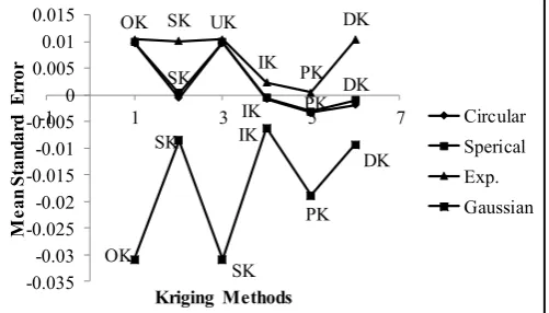
The mean standardized prediction error is shown in Figure 10. The Gaussian semivariogram with ordinary kriging and/or universal kriging had the lowest values. The exponential semivariogram with ordinary kriging had the highest positive value. The standardized mean prediction error value of the set of spherical semivariogram and simple kriging was nearest to zero and could be considered the best combination of semivariogram and kriging algorithms. The exponential semivariogram and probability kriging set of algorithms was the second best combination. The root mean square error standardized (RMSES) is shown in Figure11. The ideal set of semivariogram and kriging algorithms would have an RMSES value of 1 and be approximately equivalent to the average standard error (ASE).
24 22 20 1 8 1 6 1 4 1 2 1 0
99.9 99 95 90 80 70 60 50 40 30 20 1 0 5 1 0.1
Mean 1 7.65 StDev 1 .996 N 1 1 8 RJ 0.996 P-Value >0.1 00
Total Precipitation
P
e
rc
e
n
t
SK
PK DK OK
SK UK
DK
OK SK
UK IK
PK DK
-0.03 -0.02 -0.01 0 0.01 0.02 0.03
-1 1 3 5 7
M
e
an
Kriging Methods
Circular Spherical Exponential Gaussian
OK SK
UK
IK PK
DK
0 0.1 0.2 0.3 0.4 0.5 0.6 0.7 0.8 0.9 1
0 2 4 6
R
o
ot
M
e
an
S
q
u
ar
e
Kriging Methods
Circular
Sperical
Exponential
Gaussian
OK SK
UK
DK
OK
UK
IK PK
0 0.2 0.4 0.6 0.8 1 1.2 1.4
0 2 4 6
A
ve
rage
St
an
d
ar
d
E
rr
or
Kriging Methods
Circular Sperical Exponential Gaussian
[image:8.595.38.290.573.717.2]The best set of semivariogram and spatial interpolation algorithms is the circular semivariogram and indicator kriging. This is closely followed by the set of exponential semivariogram and indicator kriging as well as spherical semivariogram and indicator kriging respectively. The least accurate combinations were circular semivariogram and ordinary kriging, as well as circular semivariogram and indicator kriging.
[image:9.595.38.289.357.500.2]Figure 10. Graph of Mean Standardized Prediction Error of the Kriged Precipitation Data
Figure 11. Graph of Root-Mean-Mean-Square Error Standardized of the Kriged Precipitation data
DISCUSSION
Comparative Analysis of the Sets of Semivariogram-Kriging Algorithms: The decision matrix in Table 4 summarizes the performance of all 24 sets of semivariogram and kriging algorithms.
For each type of semivariogram model, the performance rating, or order of preference of the various sets of semivariogram and interpolation algorithms, are rated from 1 to 6, with 1 being the best or the most preferred and 6 being the worst or the least preferred. For instance if RMSES were used as the decision criterion, the best set of semivariogram
and spatial interpolation algorithms is the circular
semivariogram and indicator kriging and it is assigned a value of 1. The assigned values are added together and the aggregate is used to select the best set of semivariogram and interpolation algorithms. The set of semivariogram-kriging algorithms with the RMSE closest to ASE is considered as the best. The kriging – semivariogram combination which has the lowest difference between RMSE and ASE values and the lowest decision matrix aggregate value is considered the best. Thus, a plot of the relationship between RMSE and ASE should be close to 45 degrees if the set of algorithms are valid. Figure 12 depicts the relationship between RMSE and ASE values. The sets of indicator kriging and circular
semivariogram and indicator kriging and Gaussian
semivariograms could be considered the most accurate. The mean and mean standardized error values of the Gaussian semivariogram for the various kriging algorithms were quite
unstable. Thus, the indicator kriging and circular
[image:9.595.35.290.544.698.2]semivariogram algorithms could be considered as the best set for characterizing and interpolating the precipitation data.
Figure 12. RMSE – ASE Plot for Precipitation Data
Multi-scale Spatial Analysis: The precipitation data for the wet and dry months were selected for further study. ArcGIS tools were used to draw a rectangle around the state (Figure 13). The centroid of the state was calculated to be -1000 27’
46.467”and 470 33’ 48.716”. The state was divided into
OK
SK UK
IK PK
DK SK
IK PK
DK
OK SK
SK IK
PK DK
-0.035 -0.03 -0.025 -0.02 -0.015 -0.01 -0.005 0 0.005 0.01 0.015
-1 1 3 5 7
M
e
a
n
S
tan
d
ar
d
E
rr
o
r
Kriging Methods
Circular
Sperical
Exp.
Gaussian
OK
SK UK
IK
DK OK
SK UK
PK
0 0.2 0.4 0.6 0.8 1 1.2 1.4 1.6
0 2 4 6
R
oo
t-M
e
a
n
-Sq
u
a
re
St
an
d
a
rd
iz
e
d
Kriging Methods
Circular Sperical Exp. Gaussian
0 0.2 0.4 0.6 0.8 1 1.2 1.4
0 0.5 1 1.5
R
M
S
E
ASE
Circular
45 Degree
Spherical
Exponential
Gaussian Table 3. Decision Matrix Summarizing the Sets of Semivariogram and Kriging Algorithms
Circular Variogram Spherical Variogram OK SK UK IK PK DK OK SK UK IK PK DK
Mean 5 4 5 1 2 3 5 4 5 2 1 3
RMSE 4 3 4 1 2 5 4 3 4 1 2 5
ASE 3 4 3 1 2 5 3 4 3 1 2 5
MSE 5 1 5 2 4 3 5 1 5 2 4 3
RMSES 5 3 5 1 2 4 5 3 5 1 2 4
Aggregate 22 15 22 6 12 20 22 15 22 7 11 20 Exponential Variogram Gaussian Variogram OK SK UK IK PK DK OK SK UK IK PK DK
Mean 3 5 3 2 1 4 5 3 5 1 2 4
RMSE 3 4 3 1 2 5 3 4 3 1 1 5
ASE 3 5 3 1 2 4 3 4 3 1 2 5
MSE 5 3 5 2 1 4 5 2 5 1 4 3
RMSES 2 5 2 1 3 4 1 4 1 2 3 5
Aggregate 16 22 16 7 9 21 17 17 17 6 12 22
[image:9.595.311.555.561.707.2]quadrants represented by A, B, C and D (1/4th of North Dakota) and one of the four quadrants A was selected. The state was further divided into 16 quadrants (1/16th of North Dakota) and one of them A1 was selected. The centroid of
quadrant A is -1020 17’ 12.088”and 480 11’ 51.577” and that of A1 is -1030 11’ 30.686”and 480 34’ 58.531”. The wet and
dry data from the state (118 data points), 1/4th of the state, A (29 data points) and 1/16th of the state, A1 (8 data points) were
subjected to indicator kriging (using the circular variogram). Further subdivision of into smaller quadrants resulted in grids with just one or two, or no rain gauges. The kriging results in the form of maps are shown in Figures 14 and 15.
[image:10.595.309.559.185.568.2]A1 A2 A4 A3 A B D C
Figure 13. Subdivision of North Dakota Precipitation into Several Quadrants
Figure14 presents the spatial distribution maps of the wet precipitation month for North Dakota (a); 1/4th of the state, A (b); and 1/16th of the state, A1 (c) of the average monthly
precipitation for the reference period (1971-2000). The number of rain gauges n is n1 > n2 > n3 for the three conditions
considered, respectively. The top row of the Figure presents the simulated wet monthly precipitation data for North Dakota (a), while the bottom row provide simulated results for the
smaller areas for A (b) and A1 (c). Analysis of the wet monthly
precipitation along the west-east shows low precipitation at the west and higher precipitation accumulations in the eastern area of North Dakota. A similar trend is observed for the other small areas of the state considered (Figure 14 (b) and (c). In the north-south direction, a different trend of spatial distribution is exhibited; particularly in the central area of the state (a) which has high precipitation accumulations. For the smaller areas (b) and (c), the north–south longitudinal gradients of the spatial distributions of precipitation seems to be uniform. The latitudinal gradients increase along the west-east for all the three scales considered. For the dry month [Figure 15 (a), (b), and (c)] precipitation accumulations are from low to high along the west-east of the state. Along the north-south of the state, precipitation decreases from the maximum precipitation along the northern boundary to the south. This trend could be due the snow accumulation from the arctic and the large body of water in the northern part of the state. The analysis for the smaller areas (b) and (c) show a
similar trend. Thus both the wet and dry monthly precipitation have longitudinal and latitudinal accumulations are presented in Figure 3 and 4. Precipitation accumulation is affected by changes in slope in the direction, which is not the case for North Dakota which has almost a constant slope. The models were used to estimate precipitation on a regular grid for the wet and dry month (Figures 14(c) and 15(c)) and the spatial maps of precipitation produced were physically realistic. The indicator kriging and circular semivariogram produced observable patterns well and reveal a representation can be secured even for small grids.
Figure 13. Wet Month Spatial Distribution of North Dakota precipitation
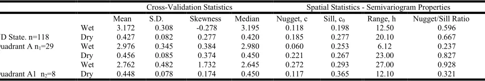
Table 5 shows the cross-validation statistics and the spatial statistics (variogram properties) for the three scales. In the case of the wet month cross-validation statistics, the mean of the state of 3.172 (n = 118) reduced to 2.976 (n1 = 29) for 1/4th of
the state and 2.762 (n2 = 8) for 1/16th of the state. The mean of
the dry month cross-validation statistics for the same scale were 0.427, 0.456, and 0.448 respectively. The standard deviation and the skewness increased for the wet month data but they followed the same trend as the mean for the dry month data. It is apparent that the degree of variation between the wet and dry months is quite significant. The nugget effect of the wet month data changed from 0.118 for the state (n1 =
118) to 0.06 for 1/4th of the state (n1 = 29) and 0.272 for 1/16th
of the state (n2 = 8). The nugget effect for the same scale
decreased from 0.185 to 0.06 and then increased to 0.272 respectively.
(a) Legend
Kriging Probability Map
[Precipitation_Data].[Jun]
Filled Contours
0 – 0.082199256
0.082199256 – 0.17487183
0.17487183 – 0.279352164
0.279352164 – 0.397144732
0.397144732 – 0.529945695
0.529945695 – 0.647738262
0.647738262 – 0.752218597
0.752218597 – 0.84489117
0.84489117 – 0.927090427
0.927090427 – 1
Precipitation_Data
ND_State (b)
Legend
Kriging Probability Map
[A_Precipitation].[Jun]
Filled Contours
0 – 0.032568067
0.032568067 – 0.084143724
0.084143724 – 0.165820303
0.165820303 – 0.295165504
0.295165504 – 0.5
0.5 – 0.704834496
0.704834496 – 0.834179697
0.834179697 – 0.915856276
0.915856276 – 0.967431933
0.967431933 – 1
A_Precipitation
A (c)
Legend
Kriging Probability Map
[A1_Precipitation].[Total]
Filled Contours
0.046111398 – 0.105302699
0.105302699 – 0.177590238
0.177590238 – 0.265871593
0.265871593 – 0.373685442
0.373685442 – 0.505353402
0.505353402 – 0.637021361
0.637021361 – 0.74483521
0.74483521 – 0.833116566
0.833116566 – 0.905404105
0.905404105 – 0.964595405
A1_Precipitation
A1
(a)
(b) (c)
[image:10.595.43.281.205.449.2]The sill for the wet month increased from 0.198 to 0.253 and 0.293 for the three scales. The sill for the dry month increased as well.
Conclusion
Forecasts from quantitative precipitation models are considered as the largest source of uncertainty in hydrologic models because of the complexity and spatial distribution of precipitation data (obtained from radar or sampling stations). Even though spatial statistics have been used to characterize and analyze precipitation data, there is a lack of knowledge of
[image:11.595.139.463.59.507.2]which kriging method and semivariogram to use. In this study six linear and nonlinear kriging techniques were paired with four semivariogram models to characterize and interpolate the precipitation data of North Dakota. The results were cross-validated and a decision matrix was developed to summarize the statistics of all the 24 combinations of kriging and variogram algorithms. The models were rated in order of preference from 1 to 6; 1 being the best and 6 being the worst. Another criteria, the difference between the RMSE and ASE was used in conjunction with the performance rating to select the best combination of kriging and semivariogram techniques. Thus the kriging – semivariogram combination, which has the
Figure 14. Dry Month Spatial Distribution of North Dakota Precipitation
Table 4. Classical Statistics and Spatial Statistics from the Multi-scale Analysis
Cross-Validation Statistics Spatial Statistics - Semivariogram Properties Mean S.D. Skewness Median Nugget, c Sill, c0 Range, h Nugget/Sill Ratio ND State. n=118
Wet 3.172 0.308 -0.278 3.195 0.118 0.198 12.50 0.596
Dry 0.427 0.082 0.277 0.420 0.185 0.277 20.10 0.667
Quadrant A n1=29 Wet 2.976 0.345 0.384 2.980 0.060 0.253 6.12 0.237
Dry 0.456 0.085 0.374 0.450 0.221 0.267 23.00 0.827
Quadrant A1 n2=8
Wet 2.762 0.482 1.732 2.645 0.272 0.293 27.00 0.928
Dry 0.448 0.078 0.174 0.450 0.117 0.365 12.10 0.321
(a)
(b)
Legend
Kriging_2
Probability Map
[Precipitation_Data].[Dec]
Filled Contours
0 – 0.132119426 0.132119426 – 0.246988413 0.246988413 – 0.346859298 0.346859298 – 0.43369034 0.43369034 – 0.509184112 0.509184112 – 0.574820887 0.574820887 – 0.650314659 0.650314659 – 0.7371457 0.7371457 – 0.837016586 0.837016586 – 0.951885573 Precipitation_Data
ND_State (b)
Legend
Kriging_2
Probability Map
[A_Precipitation].[Dec]
Filled Contours
0.109430209 – 0.202151283 0.202151283 – 0.27365543 0.27365543 – 0.328797619 0.328797619 – 0.371321881 0.371321881 – 0.404115517 0.404115517 – 0.446639779 0.446639779 – 0.501781968 0.501781968 – 0.573286115 0.573286115 – 0.666007189 0.666007189 – 0.78624074 A_Precipitation
A (c)
Legend
Kriging_2
Probability Map
[A1_Precipitation].[Dec]
Filled Contours
0.057863739 – 0.096220685 0.096220685 – 0.140337882 0.140337882 – 0.191080375 0.191080375 – 0.249443117 0.249443117 – 0.316570479 0.316570479 – 0.393778686 0.393778686 – 0.482581629 0.482581629 – 0.584720545 0.584720545 – 0.702198164 0.702198164 – 0.837317973 A1_Precipitation A1
Spatial Distribution of North Dakota Precipitation
(a)
(b) (c)
[image:11.595.61.545.564.645.2]lowest difference between RMSE and ASE values and the lowest decision matrix aggregate value, was considered the best. The indicator kriging method coupled with the circular semivariogram was considered the best set of algorithms which could be employed to characterize this precipitation data. The set of indicator kriging and circular variogram algorithms were used to investigate the effects of scale and two extreme weather seasons – dry and wet months. The centroid of the state (with 118 data points) was calculated and used to divide it into 4 quarters. One of the quarters was randomly selected to represent 1/4th of the state (29 data points). The state was further divided into 16 quarters and one of the 16 quarters was selected to represent 1/16th of the state (with 8 data points). The cross-validation statistics and variogram properties were discussed. The wet month statistics exhibited a reduction in the mean and an increase in the standard deviation with scale. The sill increased for both the wet and dry months as the scale was reduced. There was considerable degree of variation between the wet and dry months. It is suggested that more work should be done to document the effects of scale / sample size and sample locations (gridded and ungridded) on the results of models. Research in computational processes to ensure the use of better algorithms should also be advanced.
Acknowledgement: To all the authors
REFERENCES
Abtew, W., Obeysekera, J., and Shih, G. 1983. Spatial analysis for monthly rainfall in southern Florida. Water Resources Bulletin, 29 (2), 179–188.
AcrGIS ver 9.3 and 10.3, ESRI, 2015.
Ashraf, M., Loftis, JC. and Hubbard, KG. 1997. Application of geostatistics to evaluate partial weather station networks.
Agriculture. For. Meteorology. 84, 225–271.
Azimi-Zonooz, A., Krajewski, WF. Bowles, DS. and Seo, DJ. 1989. Spatial rainfall estimations by linear and non-linear
co-kriging of radar-rainfall and rain gauge data. Stochastic
Hydrology. Hydraulics. 3, 51–67.
Bacchi, B., Kottegoda, NT. 1995. Identification and calibration
of spatial correlation patterns of rainfall. Journal of
Hydrology, 165(1–4), 311-48.
Barancourt, C., Creutin, J-D., Rivoirard, J. 1992. A method for
delineating and estimating rainfall fields, Water Resources.
Research, 28 (4), 1133–1144.
Bárdossy, A. 1993. Stochastische Modelle zur Beschreibung
der raum-zeitlichen Variabilität des Niederschlages.
Mitteilungen, Institut für Hydrologie und
Wasserwirtschaft, Universität Karlsruhe, Karlsruhe, 44, 153.
Bargaoui, ZB. and Chebbi, A. 2009. Comparison of two kriging interpolation methods applied to spatiotemporal
rainfall. Journal of Hydrology, 365(1-2), 56-73.
Bedient, PB. and Huber, WC. 1992. Hydrology and Floodplain Analysis: Second Edition, Addison-Wesley, New York. Bernes, A., Delrieu, G., Boudevillain, B. 2009. Variability of
the spatial structure of intense Mediterranean
precipitation. Advances in Water Resources, 32(7),
1031-1042.
Bernes, A., Delrieu, G., Creutin, JP. and Obled, Ch. 2004. Temporal and spatial resolution of rainfall measurements
required for urban hydrology, Journal of Hydrology, 299.
Bohling. B. 2005. Estimating the risk for erosion of surface sediments in the Mecklenburg Bight (south-western Baltic Sea). Baltica, 18(1), 3–12.
Borgman, LE. 1988. New advances in methodology for
statistical tests useful in geostatistical studies.
Mathematical. Geology, 20, 383-403.
Bowman, AW. 1984. An alternative method of cross-validation for the smoothing of density estimates,
Biometrika, 71, 353-60.
Box, GEP. and Jenkins, GM. 1976. Time Series Analysis: Forecasting and Control. San Francisco: Holden Day. Bras, RL. and Rodriguez-Iturbe, I. 1985. Random Functions
and Hydrology. Addison-Wesley, Reading.
Brooker, PI. 1979. Kriging, Engineering and Mining Journal,
180(9), 148-153.
Burgess, TM. and Webster, R. 1980. Optimal interpolation and
isarithmic mapping of soil properties. I. The
semivariogram and punctual kriging. Journal of Soil
Science, 31, 315-331.
Burrough, PA. and McDonnell, RA. 1998. Principles of Geographical Information Systems. Oxford University Press, Oxford, 356.
Chilès, JP., and Delfiner, P. 1999. Geostatistics: Modeling
Spatial Uncertainty, Wiley Series in Probability and
Statistics. John Wiley & Sons, Ney York, 687.
Cressie, NAC. 1985. Fitting variogram models by weighted
least squares. Mathematical. Geology, 17, 563–586.
Cressie, NAC. 1991. Statistics for Spatial Data. Wiley, New York, 900.
Creutin, J-D., and Obled, C. 1982. Objective analyses and mapping techniques for rainfall fields: an objective
comparison. Water Resources Research, 18(2), 413–431.
Daly, C., Neilson, RP. and Phillips, DL. 1994. A statistical–
topographic model for mapping climatological
precipitation over mountainous terrain. Journal of Applied.
Meteorology, 33, 140-158.
David, M. 1977. Geostatistical Ore Reserve Estimation.
Elsevier, Amsterdam, Netherlands, 520.
Davis, J. 1987. Production of conditional simulations via the LU triangular decomposition of the covariance matrix.
Mathematical Geology, 19(2), 91-98.
Davis, J. 2002. Statistics and Data Analysis in Geology, 3rd Edition. John Wiley, New York, 656.
Delfiner, P. 1976. Linear estimation of nonstationary spatial phenomena. In: M. Guarascio, M. David and C. Huijbregts,
Editors, Advanced Geostatistics in the Mining Industry, D.
Reidel, Hingham, Massachusetts, 49–68.
Delhomme, J.-P. 1978. Kriging in the hydrosciences.
Advanced Water Resources, 1(5), 251–266.
Demyanov, V., Kanevski, M., Chernov, S., Savelieva, E., and Timonin, V. 1998. Neural network residual kriging
application for climatic data.” Journal of Geographic
Information and Decision Analysis, 2(2), 215–232.
Deutsch, CV. 1997. Petroleum Exploration, in McGraw-Hill Yearbook of Science and Technology.
Deutsch, CV. 2002. Geostatistical Reservoir Modeling, Oxford
University Press, 384.
Deutsch. CV., and Joursnel, AG. 1998. GSLIB. Geostatistical
Software Library and User′s Guide, Oxford University Press, New York, 369.
Dodson, R. and Marks, D. 1997. Daily air temperature interpolated at high spatial resolution over a large
mountainous region. Climate Research, 8(1), 1–20.