Discrete time model reference control schemes of milling forces using fractional order holds

University of Huddersfield Repository

Rubio Rodriguez, Luis and De la Sen Parte, Manuel

Discrete­time model reference control schemes of milling forces using fractional order holds

Original Citation

Rubio Rodriguez, Luis and De la Sen Parte, Manuel (2007) Discrete­time model reference control 

schemes of milling forces using fractional order holds. In: Proceedings of Industrial Electronics 

Society, 2007. IECON 2007. 33rd Annual Conference of the IEEE. IEEE, Taipei, Taiwan, pp. 798­

803. ISBN 1­4244­0783­4 

This version is available at http://eprints.hud.ac.uk/id/eprint/16030/

The University Repository is a digital collection of the research output of the

University, available on Open Access. Copyright and Moral Rights for the items

on this site are retained by the individual author and/or other copyright owners.

Users may access full items free of charge; copies of full text items generally

can be reproduced, displayed or performed and given to third parties in any

format or medium for personal research or study, educational or not­for­profit

purposes without prior permission or charge, provided:

•

The authors, title and full bibliographic details is credited in any copy;

•

A hyperlink and/or URL is included for the original metadata page; and

•

The content is not changed in any way.

For more information, including our policy and submission procedure, please

contact the Repository Team at: [email protected].

Discrete-time model reference control schemes of milling forces

using fractional order holds

L. Rubio and M. de la Sen

Instituto de Investigación y desarrollo de procesos, Universidad del País Vasco, Apdo. 644, 48940 Leioa (Spain)

[email protected]

(L. Rubio)

Abstract- Increasing competence makes to develop and implement more complex control schemes on manufacturing environments. In this paper, a discrete time model reference control for practical milling using different discretization of the continuous-time plant is presented. The different models of the scheme are obtained from a set of different discretizations of a continuous-time milling system transfer function under a fractional-order-hold of correcting gainβ∈

[ ]

−1,1

(

β−FROH

)

. The objective is to design a supervisory scheme which is able to find the most appropriate value for the gain β in an intelligent design framework. A tracking performance index evaluates each possible discretization and the scheme chooses the one with the smallest value of the index in order to generate the real control input to the plant. Two different methods of adjusting this value are presented and discussed. The first one selects it among a fixed set of possible values, while the second one the value of β is updated by adding or subtracting a small quantity.

I. INTRODUCTION

Milling is a cutting process widely used in the manufacturing of mechanical components. It is carried out by feeding a work-piece clamped on a table against a rotating multi-tooth cutter. In order to avoid machine malfunctions such as tool wear or breakage and to achieve a certain degree of quality in the finishing of the working-piece, the peak cutting force on the working piece has to be maintained below a prescribed safety upper-bound. This fact implies that a control strategy has to be implemented on the system in order to fulfill such safety and performance requirements.

Job-shops environments requires adaptive techniques since tool-part combinations are different at each operation, batch and high volume environments are characterized by fixing or varying within a known range tool-part combinations [1]. In this paper, the design of a discrete time control of milling forces is presented considering high volume operations, where the milling system model is perfectly characterized and the plant parameters are known or varied in a known way, even though sudden changes in the tool-part combinations happen.

On the other hand, different kinds of holds increase control designer attention due to their enhanced properties respect to the traditional zero order holds (ZOH), which are commonly used in manufacture floors. In this work, the strategies for controlling the milling system are based on the use of fractional order holds devices of the correcting gainβ∈

[ ]

−1,1,

(

β−FROH

)

. Then, the continuous milling system described in [2] is discretized under aβ−FROH, obtaining a series of discrete-time models of the system. The use of aβ−FROH to discretize the continuous system leads to modify the properties of the discrete zeros of the sampled

system [3,4]. Each different discretization of the plant has an associated controller [5,6].

Hence, two strategies for controlling the system, based on a fractional order hold discretization of the correcting gainβ∈

[ ]

−1,1,

(

β−FROH

)

are proposed. The objective of both strategies is to design a supervisory scheme which is able to select the most appropriate value for the gain β in an intelligent design framework. A tracking performance index evaluates each possible discretization and the scheme chooses the correcting gain leading to a smaller tracking performance index, for implementing the β−FROH device and the control law.

This fact modifies the overall closed-loop response of the system, improving, for instance, the stability of the discrete zeros or reducing the overshoot, avoiding tool breakage and tool wear and achieving the required surface on the working-piece in the milling process and better inter-sample behavior [7]. Hence, the model reference control is the designed from the so obtained scheme based discrete model.

Finally, the tracking performance of the continuous-time signal is studied. It is carried out by means of a cost function. It is applied to two cases, one when the multi-model scheme is used, and the other when just a ZOH device in a basic model reference control scheme is utilizing.

II. SYSTEM DESCRIPTION

A. Continuous-time Model

The milling system can be modeled as the series decomposition of a Computerized Numerical Control (CNC), which includes all the circuitry involving in the table movement (amplifiers, motor drives), and the tool-work-piece interaction model itself. A feed rate command f_c (which plays the role of the control signal) is sent to the CNC unit. This feed rate represents the desired velocity for the table movement. Then, the CNC unit manages to make the table move at an actual feed velocity of fa according to the CNC dynamics. Even though the machine tool drive servos are typically modeled as high order transfer functions, they can usually be approximated as a second order transfer function within the range of working frequencies [8]. Besides, they are tuned to be over-damped without overshoot, so that they can be modeled as the first order system of transfer function [2]:

( ) ( )_{( )}

1 1

+ = =

s s s c f

s a f s s G

τ (1)

constant, which depends on the type of the machine tool. In this study, it is assumed to be 0.1 ms.

In addition, the chatter vibration and resonant free cutting process can be approximated as the first order system [2]:

( ) _{( )}( ) ( ) 1 1 , , + ⋅ = = s c n N N ex st ba c K s a f s p F s p G τ φ φ (2) whereKc

(

N mm2

)

is the cutting pressure constant, b

( )

mm is the axial depth of cut, a

(

φst,φex,N

)

is a non-dimensional

immersion function, ranging from 0 to ~N(a number proportional to N) depending on the immersion angle and the number of teeth in cut, N is the number of teeth on the milling cutter and n

(

rev/s

)

is the spindle speed. The axial deep of cut function b in (2) may be time-varying leading to a potential time-varying system. In particular, it is assumed in this work that the cutting process is piecewise constant, admitting sudden changes in the cutting parameters at certain time instants, while remaining invariant between changes. This assumption allows us to consider the cutting process to be described by the transfer function (2) with the time interval between changes.

The combined transfer function of the system, obtained from (1) and (2) is

( ) _{( )}( ) ( )_{( ) ( ) ( )}

( 1)( 1)

1 1 1 + + = = + + = = = s c s m p K s c Nn ab c K s m s c A s c B s c f s p F s c G τ τ τ τ (3)

where the process gain is K_p

(

N⋅s mm

)

=K_cab Nn.

Figure 1 shows the sample work-piece depicting basic cutting geometry features with changes in the axial depth of cut used in the simulations. The spindle speed remains constant,

rpm

715 ; the work-piece is made of Aluminum 6067 whose specific cutting pressure is assumed to be 1200 ₂

mm N Kc = .

A 4-fluted carbide mill tool, full-immersed and rouging milling operation will be taken into consideration in the present paper.

Also, note that the desired final geometry of the piece to be milled involves changes in the axial deep of cut which implies suddenly changes in its value, according to the sudden changes assumption presented before. On the other hand, it has been taken into account that the control law computes new feed-rate command value at each sampling interval. Furthermore, it is worth to be mentioned that the CNC unit has its own digital position law executed at small time intervals in comparison

with the sampled time of the control law, even though if high speed milling tool drives are used [2].

B. Discrete model under β−FROH

In this paper, the problem of controlling a continuous plant is addressed by using a discrete controller. The discrete controller is obtained applying a model-reference pole-placement based control design to a discrete model of the plant (3) obtained by means of a FROH with a certain correcting gainβ . The additional “degree of freedom” β provided by the FROH can be used with a broad variety of objectives such as to improve the transient response behavior, to avoid the existence of oscillations in the continuous time output of the system or to improve the stability properties of the zeros of the discretized system [5, 10]. In this way, this work is especially focused on the use of these devices to improve the transient response of the closed-loop system by selecting an adequate value of the fractional order hold. Thus, in the following sections, a comparative study of the behavior of the closed-loop system under different values of the correcting gain is developed. Hence, the discretization of (3) under a FROH is calculated as [11]:

( )z Z

[

h ( ) ( )s G_c s

]

H_β = _β ⋅ (4)

where ( )

s sT e Ts sT e sT e s

h − −

⎟ ⎟ ⎟ ⎟ ⎠ ⎞ ⎜ ⎜ ⎜ ⎜ ⎝ ⎛ _⎟ ⎠ ⎞ ⎜ ⎝ ⎛ ₋ − + − − = 1 1 1 β β

β is the transfer

function of a β−FROH, where z is the argument of the transform

Z− , being formally equivalent to the one step ahead operators, q, used in the time domain representation of difference equations. This allows us to keep a simple unambiguous notation for the whole paper content. The sampling time T has been chosen to be the spindle speed, n, as it is usual for this kind of systems [2, 8, 11, 12]. Note that whenβ =1, theFROH hold becomes a first order hold

(

FOH

)

and when β =0, the zero order hold

(

ZOH

)

is obtained, being both particular cases of β∈

[ ]

−1,1. Furthermore,Hβ

( )

z may

be calculated using just ZOH devices in the following way:

( ) ( ) ( )

[

( ) ( )

]

( ) _{( ) ( ) =} ⎥ ⎦ ⎤ ⎢ ⎣ ⎡ − + − = ⋅ = s s c G s o h Z Tz z s c G s o h Z z z z A z z B z

H β β 1

δ β β β ( ) ⎟⎟ ⎟ ⎠ ⎞ ⎜⎜ ⎜ ⎝ ⎛ − ⋅ ⎟⎟ ⎟ ⎠ ⎞ ⎜⎜ ⎜ ⎝ ⎛ − ⋅ = c m T e z T e z z z B τ τ δ β β

(5), where ( ) s

sT e s o

h =1− − is the

transfer function of a ZOH and δ_β=1if β≠0and δ_β=0if 0

=

β , which means that a fractional order hold with β≠0 adds a pole at the origin.

C. Desired response: model reference

A second order stable system

( )

₂

2 2 2 n s n s n s m G ω ξω ω + +

= (6) is

selected to represent the system model reference. This system is characterized by a desired damping ratio, ξ and a natural

mm

87 .

5 5.87mm 5.87mm 7.55mm mm

2

mm

3 5mm 3mm

tool

[image:3.612.74.269.586.677.2]

workpiece feed

frequency, ωn. It is known that small values ofξ leads to a large overshoot and a large setting time. A general accepted range value for ξ to attain satisfactory performance is between

5 .

0 and 1, which corresponds to the so-called under-damped systems. In this way, a damping ratio of ξ =0.75and a rise time,T_r, equal to four spindle periods is usually selected for practical applications [2,13]. Furthermore, the natural frequency is then usually suggested to be rad s

r T n=2.5

ω . This

continuous-time reference model is then discretized with the same FROH as the real system was in order to obtain the corresponding discrete-time reference model for the controller. Thus, a number of different discrete models obtained from a unique continuous-time reference model are considered depending on the value of

β

used to obtain the discretization.

III. CONTROL SCHEMES DESIGNS

Milling force controllers are designed in this section using two different schemes. The design objective is to develop a closed-loop response which tracks a constant reference.

D. Basic model following scheme

The aim of the model-following control strategy is to lead the closed-loop system to behave as a prescribed reference model. Thus, the control scheme of the figure 2 is applied, where

( )

( )

( )

z R z T z ff

H = is the feed-forward compensator,

( )

( )

( )

z R z S z fc

H = is the feedback compensator,H_β

( )

z is the

discrete plant, H_m,β

( )

z is the discrete-time reference model and F_rk is the reference force.

The transfer function of the reference model is,

( )

( ) ( ) ( )

( ) ( )

( ) ( )

( ) ( )

z A z A z A z B z A z A z A z B z B z H o m o m o m o m

m = =

− '

(7)

where B_m'

( )

z contains the free-design reference model zeros,

( )

z

B− is formed by the transmitted unstable (assumed known) plant zeros and Ao

( )

z is a polynomial including the eventual

closed-loop stable pole-zero cancellations which are introduced when necessary to guarantee that the relative degree of the reference model is non less than that of the closed-loop system so that the synthesized controller is casual. A basic control scheme is displayed in figure 2. Then, polynomials

( ) ( )

z S z

R , and T

( )

z have to be synthesized (T

( )

z depends only on the reference model zeros polynomial which is of constant coefficients) where T

( )

z =B_m'

( ) ( ) ( )

z A_o z,R z (monic) and

( )

z

S are the unique solutions with degrees fulfilling

( )

,deg

( )

1,deg

(

)

2 1

degR =n S =n− A_mA_o = n− of the polynomial Diophantine equation

( ) ( ) ( ) ( )

( ) ( ) ( )

( ) ( )

z R z B

( ) ( )

zS z A

( ) ( )

z A z A z A z A z B z S z B z R z A o m o m = + ⇔ ⇔ = + − + 1 (8)

with R

( ) ( ) ( )

z =B zR1 z at every sampling instant, where n=2 if

a ZOH in view of the second order milling plant and reference model continuous-time transfer function. For FROH not being ZOH, n=3 since a new pole at the origin is automatically added to the plant.

From (7)-(8), perfect tracking is achieved through the control signal:

( )

( )

rk

( )

( )

pk k

c T_Rz_z F _RS z_z F

f _, = _, − _, (9) Two alternative organizations of the set of discrete models are proposed in this paper. The structure of both architectures is discussed in the following section.

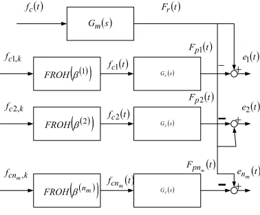
E. Multi-model scheme1

Firstly, the transfer functions composing the parallel scheme are obtained for pre-intended values ofβ . Thus, a finite set of possible design values

{

β( )1,β( )2,..,β( )nm

}

is considered,

obtaining the set of discrete transfer functions as,

( ) ( )

[

h s Gs

]

Z

H_β = _β ⋅ , β∈

{

β( )1_,β( )2_,..,β( )nm

}

Then, the actual control law at the previous time instant is applied to the above scheme by calculating the output of all the continuous time modelsF_p1

( )

t,F_p2

( )

t,..,F_pm

( )

t . The tracking performance of the set of possible models is evaluated by comparing these outputs and the desired reference output. Finally, the proposed high level supervision algorithm will select the most appropriate one to design the control law which is actually applied to the system according to the values of

( )z

H_ff H_β( )z

( )z Hfc

( )z Hm

+ε=0

[ ]KN F_rk

− +

−

c

[image:4.612.331.520.536.693.2]

f Fp

Fig.2: Basic Model following control scheme.

( )s G_m

( )t f_c

( )

( )

_β1

FROH Gc( )s

( )s Gc

( )

( )

_β2

FROH

( )s Gc

( )

( )

nm

FROHβ

( )t F_r

k c

f_1,

k c f_2,

k cnm

f _,

( )t f_c1

( )t f_c2

( )t f

m

cn

( )t Fp1

( )t Fp2

( )t F

m

pn

( )t e₁

( )t e₂

[image:4.612.67.258.599.686.2]

( )t e m n + + + −

−

−

these performance indexes. Figure 3 depicts a schematic representation of the control scheme.

F. Multi-model scheme 2

In the second criterion the system starts with an arbitrary value and its associate tracking performance is compared with the obtained from the use of other two close values ofβ. One being a slightly larger and the other slightly smaller than the active value. Then, the system only can choose a value among those three cases. However, these three potential values are not constant in general and they are updated. In case of choosing one of the two other close values to the current value ofβ . It becomes the active one and the other two are updated again by adding and subtracting a quantity. If the system chooses to maintain the same value ofβ , then the other two possible values are updated as well by considering other two closer values ofβ.

The following algorithm describes carefully this method: 1. At kthsample the active value of βisβ_k. Other two

values, β_ksup=β_k+∆β _{and β =β −∆β} k

kinf are used for simulation. Suppose that the last β switching

took place at kthsample.

2. If

(

k+1

)

T−kT ≥MT, M >0, then the tracking performance of the of the three possible discretizations are compared and one with the lowest value of the switching rule is used in the FROH device.

3. If the system chooses to maintain the same value ofβ, first ∆βis decreased and then βsupand βinfare updated. (If βk+1=βk, ∆β =∆β/m, m>1, and

β β β_ksup₊ = _k+∆

1 , βkinf+1=βk−∆β.

4. If the system chooses another value, ∆β maintains its value and βsupand βinfare calculated by adding and subtracting the following value:

- ifβ_k+1=β_ksup, β_k+ =β_k+ ∆β β_kinf₊ =β_k

1 sup

1 2 ,

- if inf

1 k

k β

β ₊ = , β_k+ =β_k β_kinf₊ =β_k −∆β

1 sup

1 ,

IV. SWITCHING RULE AND IDENTIFICATION PERFORMANCE INDEX

The objective of the supervisor is to evaluate the tracking performance of the possible controllers operating on the plant for the given reference model with the aim of choosing the current controller from the set of parallel controllers. The proposed performance index is defined as:

( )

( )

( )

( )

∑

∫

−

= −

− ₋

= k

M k j

jT

T j

pl rl

j k l

k F F d

J

1

τ τ τ

λ (10)

for1≤l<n_m, where λ∈

(

0,1

]

and M>0are design real parameters and nmis the number of possible plant

discretizations. λis a forgetting factor which allows to weight optionally more recent data ( if λ≠1 ) to the last time interval.

Note that there are two supervisory hierarchical levels of action of the intelligent system:

1. Basic control: It consists of generating the control signal from (9) for each of the discrete models integrated in the multi-model scheme.

2. Choice ofβ : The model and correcting gain β of the FROH is on-line selected via minimization of the supervisory performance index (10) and the criterion selected for choosingβ.

It is of interesting mention that the time interval between two consecutives switch times in the current controller has to be larger than a minimum residence time in order to guarantee the closed-loop stability. This value could be obtained from an ‘a priori’ knowledge or from experimental research.

V. SIMULATION RESULTS

In this section, the two above introduce control schemes are applied to the explained milling system to show the usefulness of the schemes.

Two selected plots are used tentatively for the milling system output performance evaluation. The first one uses the multi-model scheme 1letting the system to choose among any of the possible gainsβ, multi-model 1. The set of possible gains are

( )i ₌₁₋

( )

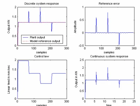
_{i−1 /10}

β for 1≤i≤15and the residence time is chosen to be one period. In the second multi-model method the initial value of ∆βis set to 0.2 and mto 2. Figures 4 and 6 show the outputs, and figures 5 and 7 the on-line active value of β selected via switching using (10), for the multi-models methods 1 and 2, respectively.

The forgetting factor is fixed to unity so that old data are not forgotten in this particular simulation package. The M value is also selected to be one. Similar results are obtained with other values of those parameters.

For the each synthesized control, four output figures are plotted in the group of figures 4 and 6. The first one depicts the model reference and the plant output signals versus sample time; the second one shows the evolution of the tracking error signal,

(

e=F_p−F_pm

)

; the third figure displays the controller response and, finally, the four graphic shows the continuous-time domain system response obtained using theβ−FROH. The figures show that the steady-state force tracks the reference force which is set to 1.2KN, except for the response peaks appreciated when the axial depth of cut, and then the transfer function, is suddenly altered. It is also appreciated that the discrete-time transient response follows exactly the discrete model reference at each sampling instant as a consequence of the perfect knowledge of the plant parameters. The programmed feed rate is feasible and smooth, even though the axial depth of cut varies.

breakage [8]. In that case, some ‘a priori’ information about the work-piece geometry is required to design a successful control, as in [14], where a CAD model of the work-piece is used to modify the control command when the axial depth of cut changes in order to minimize the overshoots due to abrupt changes in the transfer function.

VI. CONTINUOUS-TIME RESPONSES CHARACTERIZATION

In this section, the output of the milling system is evaluated under the application of the developed control schemes using fractional order holds. It is going to be compared with the output of the basic control scheme represented in section III.A under a ZOH discretization. For this purpose, a cost function is defined:

( ) ( )

( ) τ τ dτ

k

j jT

T

j pm

F p F c

J ∑n _∫

= −

− =

1 1 ,

where Fpis the output signal and Fp,mis the model reference output signal, knis the number of periods which have been taken into account in the continuous-time response characterization.

This cost function calculates an approximation of the area between the continuous-time domain system output response

and the continuous-time model reference response. The smaller this area is, the smaller cost function is, and then, the output of the system associated to the lowest value of this cost function will correspond to a signal that better follow the reference signal. In terms of milling, this fact implies better accuracy on the working-piece surface, and prevents against damaging the tool and machine tool components.

The values of the cost function are 0.0277, 0.2365 and 0.083, for the cases where multi-model scheme letting the system chooses a number of possible consideredβ - values, multi-model scheme 1, multi-multi-model changing βto a close value, multi-model scheme 2, and for the case where the model reference control is applied using a ZOH device.

The multi-model scheme 1 improves the continuous response respect to the scheme which uses just a ZOH, but the second scheme is not such efficient.

VII.CONCLUSIONS

In this paper, a multi-model discrete-time control strategy for a known continuous-time milling systems has been developed. The different discrete models are obtained by discretizing the continuous plant under a FROH device. The scheme is designed to find at each multiple of the residence

0 50 100 150 200 250 300 -0.4

-0.2 0 0.2 0.4 0.6 0.8 1

number of samples

bet

a-v

al

[image:6.612.70.293.49.219.2]

ue

Figure 4: System responses corresponding to multi-model scheme 1. Figure 5: Active value of βwith method 1.

0 100 200 300 0

1 2 3

samples

O

uput

K

N

0 100 200 300 -1

0 1 2

samples

A

m

pl

itude

0 100 200 300 0

0.5 1 1.5 2

samples

Li

near f

eed i

n m

m

/s

0 5 10 15 20 0

1 2 3

time(s)

Out

put

in

K

N

0 50 100 150 200 250 300 0

0.1 0.2 0.3 0.4 0.5 0.6 0.7 0.8 0.9 1

samples

bet

a-va

lu

[image:6.612.80.288.249.413.2]

e

time the value of the gain β which leads to the best tracking performance. Two different methods have been presented for this purpose. The first one selects the current value of the gain among a fixed set of possible prefixed values. The second one updates βonly to a close value of the current value, avoiding poor transients which may occur when the changing is big.

Simulations have showed that an appropriate choice of the value of β leads to a more precise continuous-time response than when just a ZOH is used. Moreover, the advantages and disadvantages of both methods have been discussed through a cost function which measures the continuous-time system response behavior.

On the other hand, it is of interest to mention that the general FROH device can be implemented by means of ZOH holds, which make this approach fairly feasible implemented in the manufacturing industry, see for instance [4].

ACKNOWLEDGMENT

The Authors are very grateful to Ministry of Science and Technology (MCYT) of Spain by its partial support through grant DPI2006-0714 and to Basque Government through SAIOTEK 2006 Program, Ref. S-PE06UN10. L. Rubio is also thankful to University of the Basque Country for his ph. D. studies financial support.

REFERENCES

[1] R.G. Landers, A.G. Ulsoy and Y.M. Ma, “A comparison of model-based machining force control approaches”, International Journal of Machine Tools & Manufacture, 2004, vol. 44, pp.733-748.

[2] Y. Altintas, “Manufacturing Automation”, Cambridge University Press, 2000.

[3] K.J. Astrom, P. Haganger and J. Sternby, “Zeros of sampled systems”, Automatica, Vol. 20, nº1, pp. 31-38, 1984.

[4] R. Barcena, M. De la Sen and I. Sagastabeitia, “ Improving the stability of the Zeros of Sampled Systems with Fractional Order Hold”, IEE Proc. Control Theory and Applications, 147,Vol. 4, pp. 456-464, 2000. [5] K.S. Narendra and J. Balakrishnan, “Improving Transient Response of

Adaptive Control Systems using multiple models and switching” IEEE Transaction on Automatic Control, Vol. 39, nº 9,pp.1861-1866, 1994. [6] K.S. Narendra and J. Balakrishnan, “Adaptive Control using multiple

models and switching” IEEE Transaction on Automatic Control, Vol.42, nº23,pp.171-187, 1997.

[7] Y. Altintas, I. Yellowley and J. Tlusty, “The Detection of Tool Breakage in Milling Operations”, Journal of Engineering for Industry, November 1988, Vol. 110.

[8] Y. Altintas, F. Sassani, and F. Ordubadi, “Design and Analysis of Adaptive Controllers for Milling Process. Transactions of the CSME. pp. 17-25, no. 1/2, 1990, Vol. 14.

[9] M. Ishitobi, “Stability of zeros of sampled systems with fractional order hold”, IEE Proc.-Control Theory Appl., Vol. 143, nº 3, May 1996. [10] A. Bilbao-Guillerma, M. De la Sen and S. Alonso-Quesada, “On a Root

Locus-based Analysis of the Limiting Zeros of Plants of Nominal Order at most two under FROH-discretization”, Proceedings of the 2005 American Control Conference, pp.1205-1207, June 2005, Portland, USA. [11] L.K. Lauderbaugh and A.G. Ulsoy, “Model Reference Adaptive Force Control in Milling”, Journal of Engineering for Industry, February 1988, Vol. 111.

[12] Y.H Peng,, “On the performance enhancement of self-tuning adaptive control for time-varying machining processes”, International Journal of Advanced Manufacturing Technology, pp. 395-403, 2004, 24.

[13] B.C. Kuo, (1991). Automatic Control Systems, Prentice-Hall, Englewood Cliffs, New Jersey, 1991.