Data driven approach to machine condition prognosis using least square regression trees

University of Huddersfield Repository

Tran, Van Tung

Data­driven approach to machine condition prognosis using least square regression trees

Original Citation

Tran, Van Tung (2007) Data­driven approach to machine condition prognosis using least square 

regression trees. In: The KSNVE Annual Autumn Conference, 2007, Korea. 

This version is available at http://eprints.hud.ac.uk/id/eprint/16567/

The University Repository is a digital collection of the research output of the

University, available on Open Access. Copyright and Moral Rights for the items

on this site are retained by the individual author and/or other copyright owners.

Users may access full items free of charge; copies of full text items generally

can be reproduced, displayed or performed and given to third parties in any

format or medium for personal research or study, educational or not­for­profit

purposes without prior permission or charge, provided:

•

The authors, title and full bibliographic details is credited in any copy;

•

A hyperlink and/or URL is included for the original metadata page; and

•

The content is not changed in any way.

For more information, including our policy and submission procedure, please

contact the Repository Team at: [email protected].

Data-driven approach to machine condition prognosis using least square

regression trees

Van Tung Tran

†

, Bo-Suk Yang

†

, Myung-Suck Oh

†

ABSTRACT

Machine fault prognosis techniques have been considered profoundly in the recent time due to their profit for reducing unexpected faults or unscheduled maintenance. With those techniques, the working conditions of components, the trending of fault propagation, and the time-to-failure are forecasted precisely before they reach the failure thresholds. In this work, we propose an approach of Least Square Regression Tree (LSRT), which is an extension of the Classification and Regression Tree (CART), in association with one-step-ahead prediction of time-series forecasting technique to predict the future conditions of machines. In this technique, the number of available observations is firstly determined by using Cao’s method and LSRT is employed as prognosis system in the next step. The proposed approach is evaluated by real data of low methane compressor. Furthermore, the comparison between the predicted results of CART and LSRT are carried out to prove the accuracy. The predicted results show that LSRT offers a potential for machine condition prognosis.

Key Words: Least square method; Embedding dimension; Regression trees; Prognosis; Time-series forecasting

1.

Introduction

Most of the components in machine are degraded condition during operation due to wear which is the major reason causing machine breakdown. Maintenance is the set of activities performed on a machine to sustain it on operable condition. The most common maintenance strategy is the corrective maintenance which almost means “fix it when it breaks”. However, this strategy reduces the availability of machine and high unscheduled downtime. Condition-based maintenance (CBM) which involves diagnostic module and prognostic module is an alternative. Prognosis is the ability to access the current state, forecast the future state, and predict accurately the time-to-failure or the remaining useful life (RUL) of a failing components or subsystems. RUL is the time left for the normal operation of machine before the breakdown occurs or machine condition reaches the critical failure threshold.

Prognosis is a relatively new area and becomes a significant part of CBM [1]. Various approaches to prognosis have been developed that range in fidelity from simple historical failure rate models to high-fidelity physics-based models. Fig. 1 illustrates the hierarchy of potential prognostic approaches related to their applicability and relative accuracy as well as their complexity. Each of those approaches has advantages and limitations in application. For example, experience-

P ro

g n o s tic

a_p p ro

a_c h

In

cr

e

a

si

n

g

co

st

a

n

d

a

ccu

ra

cy

Fig.1 Fidelity of prognostic approaches

based prognosis is the least complex, however, it is only utilized in situations where the prognostic model is not warranted due to low failure occurrence rate; trend-based prognosis may be implemented on the subsystems with slow degradation type faults [2].

Data-driven and model-based techniques are much considered due to their accuracy. Nevertheless, model-based techniques require accurate mathematical models of failure modes and are merely applied in some specific components in which each of them needs different model. Furthermore, a suitable model is also difficult to establish to mimic the real life. Meanwhile, data-driven techniques can generate the flexible and appropriate models for almost failure modes. Consequently, data-driven approaches are firstly examined that some of those have been proposed [3-6].

In order to predict the condition of machines, one-step-ahead or multi-one-step-ahead predictions of time-series

† Pukyong National University, Korea. E-mail : [email protected]

2 forecasting techniques is frequently used. They imply that the prognostic system utilizes available observations to forecast one value or multiple values at the definite future time. The more the steps ahead are, the less reliable is the forecasting operation because multi-step prediction is associated with multiple one-step operations [6].

In data-driven approaches, the number of essential observations, so-called embedding dimension d,is used for forecasting the future value. It should be chosen large enough so that the estimator can forecast accurately the future value and not too large to avoid the unnecessary increase in computational complexity. False nearest neighbor method (FNN) [7] and Cao’s method [8] are commonly used to determine the embedding dimension. However, FNN method not only depends on chosen parameters and the number of available observations but also is sensitive to additional noise. Cao’s method overcomes the shortcomings of the FNN approach and therefore, it is chosen in this study.

The CART [9] is widely implemented in machine fault diagnosis. In the prediction techniques, CART is also applied to forecast the short-term load of the power system [10]. Nevertheless, the average value of samples in each terminal node used as predicted result is the reason for reducing the accuracy of CART. Several approaches have been proposed to ameliorate that CART’s limitation [12-14]. In this article, we suggest the use of LSRT which is an extension of the CART as an estimator for predicting the conditions of machine.

2.

Background knowledge

2.1 Determine the embedding dimension

Assuming a time-series of x1, x2, …, xN. The time

delay vector is defined as follows:

τ τ τ τ ) 1 ( ,..., 2 , 1 ] ..., , ,

[ 2 ( 1)

) ( − − = = − + + + d N i x x x x

y_{id i i i i d}

(1)

where τ _{is the time delay. Defining the quantity as}

follows: ) ( ) ( ) 1 ( ) 1 ( ) , ( ) , ( ) , ( d y d y d y d y d i a d i n i d i n i − + − + = ₍₂₎

where ||⋅_{|| is the Euclidian distance and is given by the}

maximum norm, yi(d) means the ith reconstructed vector and n(i, d) is an integer such that yn(i,d)(d)is the nearest

neighbor of yi(d) in the embedding dimension d. In order to avoid the problems encountered in FNN method, the new quantity is defined as the mean value of all a(i, d)’s:

∑

− = − = τ τ d N i d i a d N d E 1 ) , ( 1 ) ( (3)

E(d) is dependent on only the dimension d and the time delay τ_{. To investigate its variation from} d to d+1, the parameter E1 is given by

) ( ) 1 ( ) ( 1 d E d E d

E = + ₍₄₎

By increasing the value of d, the value E1(d) is also

increased and it stops when the time series comes from a deterministic process. If a plateau is observed for d ≥ d0, d0 + 1 is the minimum embedding dimension.

The Cao’s method also introduced another quantity

E2(d) in case that E1(d) is slowly increasing or has

stopped changing if d is large enough:

) ( ) 1 ( ) ( 2 d E d E d E ∗ ∗ + = ₍₅₎ where

∑

− = + + − − = τ τ τ τ d N i d d i n d i x x d N d E 1 ) , ( * 1 ) ( (6)

2.2 Least square regression trees

The CART [16] involves classification tree and regression tree. The classification tree deals with a qualitative output variable whilst the regression tree handles a quantitative one. Given a data set comprised n

couples of observation (y1,x1),...,(yn,xn) , where

) ,...,

( 1i di

i = x x

x is a set of independent variables and

R

y_i∈ _{is a response associated with} xi, the regression

tree is constructed by using recursively partitioning process of this data set into two descendant subsets which are as homogeneous as possible until the terminal nodes are achieved.

The split values for partitioning process are chosen so that the sums of square errors are minimum. The sum of square error of the tth subset is expressed as:

2 , )) ( ( 1 ) (

∑

∈ − = t y i i i t y y n t R x (7)

In the LSRT, the average of response at any node is replaced by the local model f(θ,xi)which shows the

relationship between the response yi and a set of independent variable xi. Hence, the sum of square error

of the tth node (subset) can be rewritten as:

2 , )) , ( ( 1 ) (

∑

∈ − = t y i i i i f y n t R x x θ ₍₈₎

where θθθθ_{is a set of parameters. The local models ( , )}

i f θ x

can be either linear or non-linear model in which the forms are known with unknown values of parameters as shown in Table 1

Table 1 Local model types in LSRT

Model type Description Parameters

Polynomial

∑

+ = − + = 1 1 1 n i i n ix y θ i θ Power 3 2 2 1 1 θ θ θ θ θ x y x y + = = 3 2 1,θ ,θ

θ Fourier

∑

∑

= = + + = n i n i x n x n y i i 1 2 1 1 0 ) sin( ) cos( ω θ ω θ θ i i 2 1 0,θ ,θ θ

Sine

∑

=

+ =

n

i i i i

x y

1

3 2

1sin(θ θ )

θ

i i i 2 3

1,θ ,θ θ

Those local models are organized as a set of models. At any node, the values of parameters of each model are initially calculated by using least square method [11], the fit model are subsequently chosen based on the sum of squares due to error (SSE) and the root mean squared error (RMSE) criterions:

∑

∑

= = − = − = n i i i n i i i y y n RMSE y y SSE 1 2 1 2 ) ˆ ( 1 ) ˆ ( (9)

where yi andyˆ are response value and predicted value i

given by local model at that node, respectively. Consequently, the outputs of terminal nodes are local models that lead to more accurate prediction.

Similarly to CART, LSRT is also pruned in order to avoid the overfitting and complicated problems. In this work, we use 10 cross-validations to select the best tree size.

3.

Proposed system

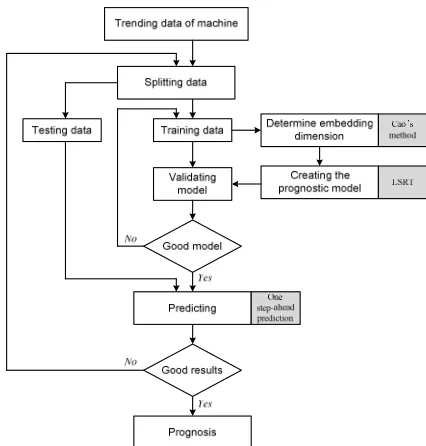
[image:4.595.322.535.199.422.2]

Normally when a fault occurs, the conditions of machine can be identified by the change in vibration amplitude. In order to predict the future state based on available vibration data, the proposed system as shown in Fig. 2 which consists of four procedures is proposed.

Fig. 2 Proposed system for machine fault prognosis.

The role of each procedure is explained as follows:

Step 1 Data acquisition: acquiring vibration signal during the running process of the machine until faults occur.

Step 2 Data splitting: the trending data is split into two parts: training data for building the model and testing data for testing the validated model.

Step 3 Training-validating: determining the

embedding dimension based on Cao’s method, building the model and validating the model for measuring the performance capability.

Step 4 Predicting: one-step-ahead prediction is used to forecast the future value. The predicted result is measured by the error between predicted value and actual value in the testing data. If the prediction is successful, the result obtained from this procedure is the prognosis system.

4.

Experiments and results

4

Male rotor axial Male rotor horizontal

Motor DE/NDE horizontal

Motor DE/NDE vertical

Motor DE/NDE axial Male rotor vertical

Suction vertical, horizontal, axial

Symptom sensing

CMS Off-line monitoring (100mV/g acceleration)

[image:5.595.321.520.97.264.2]

CMS Off-line monitoring (100mV/g acceleration) (Only horizontal)

[image:5.595.79.295.99.222.2]

Fig. 3 Low methane compressor.

Table 2 Description of system

Electric motor Compressor Voltage 6600 V Type Wet screw

Power 440 kW

Lobe

Male rotor (4 lobes)

Pole 2 Pole Female rotor

(6 lobes)

Bearing NDE:#6216, DE:#6216

Bearing

Thrust: 7321 BDB

RPM 3565 rpm Radial: Sleeve type

The data applied in this study is peak acceleration and envelope acceleration trending data recorded from August 2005 to November 2005 as shown in Figs. 4 and 5. Consequently, it can be seen as time-series data.

The machine is in normal condition during the first 300 points. After that time, the condition of machine suddenly changes indicating some faults occurring in this machine. With the aim of forecasting the change of machine condition, the first 300 points were used to train the system and the following 200 points were employed for testing system.

[image:5.595.60.294.99.375.2]

Fig. 4 The entire of peak acceleration data of low methane compressor.

Fig. 5 The entire of envelope acceleration data of low methane compressor.

The predicting performance is evaluated by using the RMSE given in Eq. (9). The time delay value is chosen as 1 for the reason that one step-ahead is implemented in all datasets. The embedding dimension is estimated to be 6 when the values of E1(d) reaches its saturation as

depicted in Fig. 6.

Fig. 6 The values of E1 and E2 of peak acceleration

data of low methane compressor.

0 50 100 150 200 250 300

0.34 0.36 0.38 0.4 0.42 0.44 0.46

Number of data

A

c

c

e

le

ra

ti

o

n

(

g

)

RMSE = 0.0011883

Actual Predicted

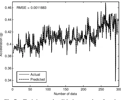
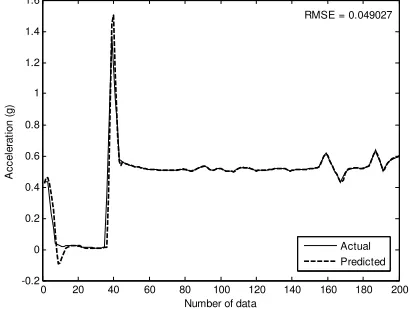
[image:5.595.324.533.381.528.2] [image:5.595.70.273.540.703.2] [image:5.595.324.522.566.730.2]

Fig. 7 depicts the training and validating results of peak acceleration data with a small RMSE value of 0.00118. In testing process, the independent data set contained the changing machine condition is used. Fig.8 shows the actual-like predicted results with the RMSE error of 0.049027 although the predicting model was not trained with those changing values. That is impossible to obtain with CART as shown in Fig. 9.

0 20 40 60 80 100 120 140 160 180 200 -0.2

0 0.2 0.4 0.6 0.8 1 1.2 1.4 1.6

Number of data

A

c

c

e

le

ra

ti

o

n

(

g

)

RMSE = 0.049027

[image:6.595.64.280.197.562.2]

Actual Predicted

Fig.8 Predicted results of peak acceleration data using LSRT.

0 20 40 60 80 100 120 140 160 180 200 0

0.2 0.4 0.6 0.8 1 1.2 1.4

Number of data

A

c

c

e

le

ra

ti

o

n

(

g

)

RMSE = 0.18546

[image:6.595.69.274.206.367.2]

Actual Predicted

[image:6.595.75.281.399.564.2]

Fig.9 Predicted results of peak acceleration data using CART.

Table 3 The RMSE of CART and LSRT

Data type Training Testing

CART LSRT CART LSRT

Peak

acceleration 0.00062 0.0011 0.1855 0.049

Envelop

acceleration 0.00028 0.00015 0.1429 0.101

Table 3 shows not only the remaining results of applying LSRT on envelop acceleration data but also the comparison of the RSME between CART and LSRT. According to table 3, training results of CART are sometimes slightly smaller than those of LSRT but the testing results of CART are always larger. This shows the superior of LSRT in aspect of machine condition

prognosis.

5.

Conclusions

Machine condition prognosis is extremely significant in foretelling the degradation of working condition and trends of fault propagation before they reach the alarm. In this study, the least square regression tree together with one-step-ahead of time-series techniques have been investigated for machine condition prognosis. The proposed method is validated by predicting future state condition of a low methane compressor wherein the peak acceleration and envelope acceleration have been examined. The obtained results confirm that the proposed method offers a potential for machine condition prognosis with one-step-ahead prediction.

References

(1) Jianhui Luo, M. Namburu, K. Pattipati, Liu Qiao, M. Kawamoto, S. Chigusa, Model-based prognostic techniques, AUTOTESTCON Proceedings, IEEE Systems Readiness Technology Conference, 22-25 Sept. (2003) 330–340.

(2) M. J. Roemer, C. S. Byington, G. J. Kacprzynski, G. Vachtsevanos, An overview of selected prognostic technologies with application to engine health management, Proceedings of GT2006, (2006).

(3) G. Vachtsevanos, P. Wang, Fault prognosis using

dynamic wavelet neural networks, AUTOTESTCON

Proceedings, IEEE Systems Readiness Technology Conference, 22-23 Aug. (2001) 857–870.

(4) R. Huang, L. Xi, X. Li, C. R. Liu, H. Qiu, J. Lee, Residual life prediction for ball bearings based on self-organizing map and back propagation neural network methods, Mechanical Systems and Signal Processing 21 (2007) 193–207. (5) W.Q. Wang, M.F. Golnaraghi, F. Ismail, Prognosis of machine health condition using neuro-fuzzy system, Mechanical System and Signal Processing 18 (2004) 813–831.

(6) W. Wang, An adaptive predictor for dynamic system forecasting, Mechanical Systems and Signal Processing 21 (2007) 809–823

(7)M.B. Kennel, R. Brown, H.D.I. Abarbanel, Determining embedding dimension for phase-space reconstruction using a geometrical construction, Physical Review A 45 (1992) 3403– 3411.

(8)L. Cao, Practical method for determining the minimum embedding dimension of a scalar time series, Physica D 110 (1997) 43–50.

(9)L. Breiman, J.H. Friedman, R.A. Olshen, C.J. Stone, Classification and regression trees, Chapman & Hall (1984).

(10) J. Yang, J. Stenzel, Short-term load forecasting with increment regression tree, Electric Power Systems Research 76 (2006) 880–888

(11) R. Johansson, System modeling and identification, Prentice-Hall International, Inc., (1993).

(12) A. Suárez, J.F. Lutsko, Globally optimal fuzzy decision trees for classification and regression, IEEE Transactions on Pattern Analysis and Machine Intelligence 21 (1999) 1297-1311.

[image:6.595.51.292.609.682.2]

6

24 (2003) 75-90.