Improved Rate Control Algorithm Based on R  Model in High Efficiency Video Coding

ISBN: 978-1-60595-520-9

 

Improved Rate Control Algorithm Based on R-



Model in High

Efficiency Video Coding

He XU

*

_{, Qiang LI and Yan MING}

Chongqing Key Laboratory of Signal and Information Processing, Chongqing University of Posts and Telecommunications, Chongqing 400065, P.R. China

*Corresponding author

Keywords: HEVC, Rate control, R- model, Image complexity, Parameter update.

Abstract. In order to improve the accuracy of rate control for High Efficiency Video Coding, the paper proposed an improved rate control algorithm based on R- model. First of all, it exploits G and MAD weighting to represent the complexity of the LCU layer image. Afterwards, it utilizes the feedback information of the encoded units to further adjust the quantization parameters. Eventually, the model parameters are updated by using video coding distortion and Newton method. Experimental results illustrate that the average Bit-error of the improved algorithm reduces by 0.055%, and the average luminance peak signal to noise ratio increases by 0.07dB compared with rate control algorithm for the current HEVC.

Introduction

In April 2013, JCTVC enacted a new generation of video coding standards High Efficiency Video Coding[1]_{. The application foreground of HEVC has attracted much attention of video consumers}

and video content integration service providers. At present, transmission bandwidth and storage space are still the most critical resources in video applications. How to obtain the best video experience in the limited storage space and transmission channel has been the untiring pursuit of experts, scholars and video content providers. If the output bitstream of video coding is too big, it will block the transmission channel up. It will lead to delaying video transmission or lost frames. If the output bitstream is too small, it will reduce video quality of the decoder. The main method to solve this problem is to use rate control technology, i.e., the video coding bits is adjusted reasonably, and the size of video output bitstream is adjusted so that the video coding quality can be the best under the condition of video transmission. Hence, rate control algorithms are used in the H. 263[2]_,

H.264/AVC and HEVC standards to meet the needs of video coding practical applications.

As to the R- model in JCTVC-K0103[3] _{proposal rate control algorithm of HEVC, it is defined}

that we can obtain Lagrange multiplier through the rate distortion model, then we will obtain actual quantization parameters according to the relationship between  and quantization parameters. The rate control effect of R- model rate control algorithm is better than the R-Q model, and its fluctuation is smaller. However, as for those intensely moving video sequences, this algorithm lead to allocating bits in the LCU layer inaccurately and losing the peak signal to noise ratio of image.

An improved rate control algorithm used weighted spatial and temporal information and model parameter update is proposed in the paper. Firstly, the algorithm guides the bits allocation in LCU layer by weighing the local kinematically spatial complexity and the temporal complexity of the global motion in this layer. Secondly, the video distortion and Newton method [4] _{are used to}

The Optimization Strategies of R- Model Rate Control Algorithm Optimization of LCU Layer Complexity Measures

The gradient G of image reflects the spatial location information of every pixel, and it can accurately represent the complexity of image content. The gradient G in LCU layer is calculated as fllows:

  



  







∑∑

1 ，

1 1

1

1 1

1 H -= i

-W

= j

j i, I -j i, I + j i I -j i, I W

× H =

G   (1)

Where H _and W are the height and width of one LCU, and I

 

i,j is the pixel value at position

 

i,j .

The MAD in LCU layer is calculated as fllows:

   

W × H

| j i, I -j i, I | = MAD

-H

= i

-W

=

j cur pred

∑∑

1

1 1

1 (2)

 

i j

Icur , is the pixel value of the original signal at position

 

i,j , and Ipred i,j is the pixel value of

predicted signal at position

 

i,j . The time correlation is used in the MAD _{prediction, the relative}

information of intra frames can be well reflected, while the gradient G _{reflects the spatial}

correlation of pixels. Therefore, the idea of space time weighted combination is used in the paper, i.e., the weighted MAD _and G _{is used to estimate the complexity of the current LCU.}

As to the insufficient of R- model rate control in JCTVC-K0103 proposal, an new complexity NC is obtained by using the LCU layer space time complexity of weighted joint in the paper according to the unique characteristics of the HEVC. The NC can effectively distinguish the LCU with different complexity, and it can be well fitted with the actual complexity, i.e., they are the linear relationship. Therefore, the algorithm will allocate the target bits more reasonable according to complexity of the LCU layer which is got by a weighted combination method. After a large number of experimental statistical analysis, the NC is calculated as follows:

G × + MAD =

NC 0

.

1 ₍₃₎

LCU Layer Quantization Parameter Adjustment Factor

The quantization parameter of the current LCU are calculated according to its image complexity. If the LCU complexity is changed, its quantization parameter will be adjusted. Because the QPvalue

of the LCU in I frame is a setting value of initial QP in the configuration file, the QPvalue saty

the same. For other frames, an adjustment factor of the formula (4) is defined based on the complexity of the current LCU prediction and gradient values G. The quantization parameter QP

obtained by the calculation of current LCU is adjusted by AF.

G NC =

AF (4)

Model Parameter Update

The rate control model parameters  _and  of rate control model are calculated by Newton iteration after the video distortion is known. Newton method is usually used to solve the optimization problem, the basic idea of solving the problem is as follows. The objective function is expanded at the minimum point, then the zero of first derivative in the objective function will be obtained, i.e., it is the estimated value of minimum point. Assume the objective function is f x , the

   xn f n x f -n x = 1 + n

x _{ (5)}

Where x_n and xn1 represent the nth iteration point and the No(n1) iteration point.  f

 

xn

and f

 

xn represent first-order derivative at point and second derivative at point of the objective

function.

When video is encoded by the parameter C_{old and} Kold, the video coding distortion at the target

bitrate R _{is as follows.}

old

K old old C R

D    (6) Assume actual bit rate after video coding is R_real, the actual distortion is Dreal.

K real real C R

D    (7) Take natural logarithms on both sides of formula (8), and assume ClnC_.

real real C K R

D ln

ln   (8) Therefore, the square error between the actual coding distortion and the coding distortion obtained by target rate estimation is as follows.





2

2 _{ln ln} old real D

D

e   (9) Combine formula (8) and formula (9), the results are as follows.





2

2 _{ln ln}

old real D R

K C

e    (10) Take _e2 _{the first-order and second derivative of the}

C and K, and use the Newton iterated

method.



real old



old

new C D D

C    ln ln (11)

real old real old new _R D D K K ln ln ln  

 (12)

Take natural logarithms on (11), and combine taking the exponent and the Taylor expansion for it.







real old



old

new C D D

C  1 ln ln (13) There are two formulas as follows.

       1 old old old old old K β K C α (14)        1 new new new new new K β K C α (15)

In the formulas, αnew and βnew represent the model parameters when we determine quantization

parameters, while αnew _and βnew _{are updating values.}

Combine formula (12), formula (13), formula (14), and formula (15), what’s more, the antilogarithm of logarithm keep positive, the results are as follows.

real old old real

old

new _R

β Rλ -D β

β

ln 1 ln

ln _

  

  

 

 (17)

Formula (16) and formula (17) are the final model parameters updated formulas. Where

λ

_{old is}

the Lagrange factor of the current encoded unit. Since the update part of the model parameters takes full advantage of the information of the relevant coding parameters, the accuracy of rate control is improved.

Improved Rate Control Algorithm Based on R- Model Target Bit Allocation of Picture Group GOP

The target bits of any frame is calculation by formula (18).

f

R

R

_AvgPic



(18)

Where f and R _{represent the frame rate and target bits.}

The target bits allocation of Group Of Pictures layer[5] _{are as follows.}





SW

R SW N

R

T AvgPic coded coded AvgPic

  



(19)

GOP AvgPic

GOP

T

N

T





(20) Where T_AvgPic represent mean target bits of every picture, TGOP represent target bits of every GOP,

coded

N represent number of the coded pictures. Rcoded is the bit cost for all the coded pictures. NGOP is

the number of pictures in a GOP. SWrepresent the size of the sliding window which is set to 40. Target Bit Allocation of Frame Layer

The current target bits[11] _{are calculated by formula (21).}







 



ctures NotCodedPii

CurrPic GOPcoded

GOP

curPic T R _ω ω

T (21)

GOPcoded

R _{represent the number of bits coded in the current GOP.}

ω

_{i represent weight of picture}

level bit allocation. ωCurrPic represent weight of picture level bit allocation for current picture. TGOP

represent target bits of a GOP. NotCodedPictures _{represent uncoded picture numbers.} Target Bit Allocation of LCU Layer

Because the less bits are allocated in the latter LCU, an improved LCU level bit allocation algorithm which is proposed in the paper can make the bit allocation reasonably. The algorithm use formula (3) to get the new complexity NC, which can measure the image complexity in LCU layer.

Furthermore, this algorithm regard NC _{as allocated weight. The calculation formula of target bits}

in LCU layer are as follows.









 



CUs NotCodedL

i

CurrLCU Piccoded

headbits CurrPic

CurrLCU

NC NC R

T T

T (22)

Where T_CurrPic represent the target bits of current frame. T_{headbits represent the estimated head bits.}

Piccoded

R _{represent the number of bits coded in the current picture.} NC_{i represent the weight of LCU}

of LCU layer.

Adjustment of LCU Layer Quantization Parameters

After the target bits of each layer are obtained, the quantization parameter QP _and λ _{will be}

obtained by the R- model, the calculation formula is as follows.

β

bpp

α

λ  (23)

7122 13 ln 2005

4. λ .

QP   (24) The initial values of  and  are set to 3.2003 and -1.367 respectively[6]_.

The first section shows that we need to readjust the QP _{of current LCU. According to the}

statistical analysis of amounts of experimental data, the algorithm will adjust the QP _value

according to the formula (25).

      

 

  

  

 



3 0 2

3 0 2

0 1

2 0 15

0 1

15 0 2

. AF QP

. AF . QP

. AF . QP

. AF QP

QP (25)

Updating of Model Parameters

The model parameters are updated according to formula (16) and formula (17). Update of Buffer Occupancy

After a picture is encoded, the formula (26) is used to update the buffer occupation.

f R R B

Bc  old  real  (26)

real

R _{is the actual encoding consuming of the current frame.} R _{is previously setted channel}

bandwidth, i.e., the initial target bitrate. f _{is the frame rate.}

The Process of Improved Rate Control Algorithm Based on R- Model

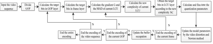
[image:5.612.87.528.514.605.2]

The process of improved rate control algorithm based on R- model in this paper is as shown in Figure 1.

Figure 1. Rate control flowcharting of the paper.

The description of this algorithm is as follows.

(1)Input the video sequence and divide the sequence into GOP according to the value of the GOPSize in the encoding configuration file.

(2)If it is I frame, encoding is executed according to the initial QP of encoding configuration

file. If it is P frame, the target bits in GOP layer are obtained by the formula (18) ~ (20). (3)The target bits in frame layer are obtained by formula (21).

(5)The target bits in LCU layer are obtained by formula (22) and the new complexity of current LCU which is got by formula (3) .

(6)The quantization parameters are obtained by formula (24). The encoding is executed by formula (25) after fine-tuning.

(7)After a LCU is encoded completely, the model parameters of the R- are updated according to the formula (16) and the formula (17), then returned (3), the next step is executed until the current frame is encoded completely.

(8)The buffer occupation Bc is updated by formula (26), then return (2), the next step is

executed until the current GOP is encoded completely.

(9)Returns (1) until the entire sequence encoding is completed.

Experimental Results and Analysis

The control accuracy and coding performance of this improved rate control algorithm which is proposed in the paper are tested in HEVC reference software HM10.0[7]_{. The tested coding}

configuration file is LD configuration file used IPPP coding structure. The configuration file of test sequences and coding configuration file are from JCTVC Common Test Conditions[8]_{. The basic}

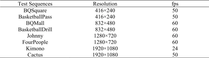
[image:6.612.129.481.324.423.2]

information of test sequence is as follows. Each test sequence will be encoded with 100 frames.

Table 1. Basic information of test sequences.

Test Sequences Resolution fps

BQSquare 416×240 50

BasketballPass 416×240 50

BQMall 832×480 60

BasketballDrill 832×480 60

Johnny 1280×720 60

FourPeople 1280×720 60

Kimono 1920×1080 24

Cactus 1920×1080 50

Under the same configuration conditions, the performance of three algorithms that they are the rate control algorithm of JCTVC-K0103 proposal and this paper are tested. The test specifications are bit-error, increment of peak signal to noise ratio in image luminance compent Y, ΔY-PSNR,

BDBR and BDPSNR[9]_{. The calculation formula of}

error

-Bit _and ΔY-PSNR _{are formula (27) and}

formula (28) respectively.

% 100 | |

  

R R R error

-Bit real (27)

In the formula (27), R_realis actual bit rate which is used the rate control algorithm. Ris the target

bit rate.

K0103 -JCTVC real Y -PSNR PSNR

-Y PSNR

-Y  

 (28)

real PSNR

-Y _{is the actual luminance component peak signal to noise ratio of the image which is}

used the rate control algorithm. Y-PSNR_{JCTVC-K0103 is the luminance component peak signal to noise}

ratio of the image which is used the JCTVC-K0103 rate control algorithm.

[image:7.612.86.530.79.701.2]

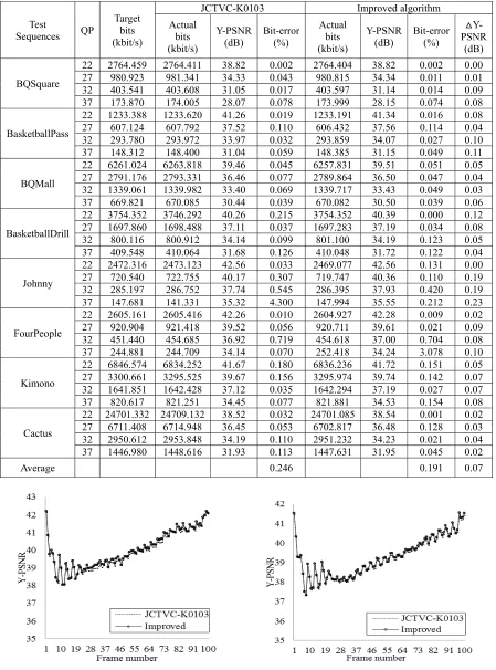
Table 2. Comparison of the JCTVC-K0103 algorithm with the improved algorithm.

Test

Sequences QP

Target bits (kbit/s)

JCTVC-K0103 Improved algorithm Actual

bits (kbit/s)

Y-PSNR

(dB) Bit-error (%)

Actual bits (kbit/s)

Y-PSNR

(dB) Bit-error (%)

ᇞY- PSNR

(dB)

BQSquare

22 2764.459 2764.411 38.82 0.002 2764.404 38.82 0.002 0.00 27 980.923 981.341 34.33 0.043 980.815 34.34 0.011 0.01 32 403.541 403.608 31.05 0.017 403.597 31.14 0.014 0.09 37 173.870 174.005 28.07 0.078 173.999 28.15 0.074 0.08

BasketballPass

22 1233.388 1233.620 41.26 0.019 1233.191 41.34 0.016 0.08 27 607.124 607.792 37.52 0.110 606.432 37.56 0.114 0.04 32 293.780 293.972 33.97 0.032 293.859 34.07 0.027 0.10 37 148.312 148.400 31.04 0.059 148.385 31.15 0.049 0.11

BQMall

22 6261.024 6263.818 39.46 0.045 6257.831 39.51 0.051 0.05 27 2791.176 2793.331 36.46 0.077 2789.864 36.50 0.047 0.04 32 1339.061 1339.982 33.40 0.069 1339.717 33.43 0.049 0.03 37 669.821 670.085 30.44 0.039 670.082 30.50 0.039 0.06

BasketballDrill

22 3754.352 3746.292 40.26 0.215 3754.352 40.39 0.000 0.12 27 1697.860 1698.488 37.11 0.037 1697.283 37.19 0.034 0.08 32 800.116 800.912 34.14 0.099 801.100 34.19 0.123 0.05 37 409.548 410.064 31.68 0.126 410.048 31.72 0.122 0.04

Johnny

22 2472.316 2473.123 42.56 0.033 2469.077 42.56 0.131 0.00 27 720.540 722.755 40.17 0.307 719.747 40.36 0.110 0.19 32 285.197 286.752 37.74 0.545 286.395 37.93 0.420 0.19 37 147.681 141.331 35.32 4.300 147.994 35.55 0.212 0.23

FourPeople

22 2605.161 2605.416 42.26 0.010 2604.927 42.28 0.009 0.02 27 920.904 921.418 39.52 0.056 920.711 39.61 0.021 0.09 32 451.440 454.685 36.92 0.719 454.618 37.00 0.704 0.08 37 244.881 244.709 34.14 0.070 252.418 34.24 3.078 0.10

Kimono

22 6846.574 6834.252 41.67 0.180 6836.236 41.72 0.151 0.05 27 3300.661 3295.525 39.67 0.156 3295.974 39.74 0.142 0.07 32 1641.851 1642.428 37.12 0.035 1642.294 37.19 0.027 0.07 37 820.617 821.251 34.45 0.077 821.881 34.53 0.154 0.08

Cactus

22 24701.332 24709.132 38.52 0.032 24701.085 38.54 0.001 0.02 27 6711.408 6714.948 36.45 0.053 6702.817 36.48 0.128 0.03 32 2950.612 2953.848 34.19 0.110 2951.232 34.23 0.021 0.04 37 1446.980 1448.616 31.93 0.113 1447.631 31.95 0.045 0.02

Average 0.246 0.191 0.07

Figure 2. Y-PSNR comparison diagram of Johnny. Figure 3. Y-PSNR comparison diagram of FourPeople.

[image:7.612.83.532.82.688.2]

[image:8.612.143.472.113.238.2]

terminal is also different. The Y-PSNR is increased slightly compared with the JCTVC-K0103 rate control algorithm.

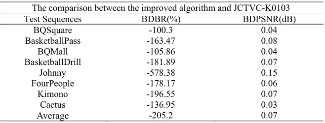
Table 3. Encoding RD performance comparation of the improved algorithm. The comparison between the improved algorithm and JCTVC-K0103 Test Sequences BDBR(%) BDPSNR(dB)

BQSquare -100.3 0.04

BasketballPass -163.47 0.08

BQMall -105.86 0.04

BasketballDrill -181.89 0.07

Johnny -578.38 0.15

FourPeople -178.17 0.06

Kimono -196.55 0.07

Cactus -136.95 0.03

Average -205.2 0.07

Table 3 and Table 4 are the rate distortion performance comparison between this proposed algorithm in the paper and the other two algorithms. The test specifications are BD-PSNR and BDBR. As to Table 3, we can see that the improvement of the rate distortion performance which this improved algorithm in the paper compare with the JCTVC-K0103 rate control algorithm is greater, i.e., the average BD-PSNR increases by 0.07dB under the LD configuration.

The RD (Rate Distortion) performance curve of the rate control algorithm in this paper and the JCTVC-K0103 proposal are as follows. The A of Figure 4 and Figure 5 is the JCTVC-K0103 algorithm. The B of Figure 4 and Figure 5 is the rate control algorithm in this paper.

[image:8.612.106.515.313.457.2]

Figure 4. RD curves of Johnny sequence. Figure 5. RD curves of FourPeople sequence.

As for Figure 4 and Figure 5, we can see that the RD performance curve of the proposed algorithm is over the curve of JCTVC-K0103 algorithm. It shows that the Y-PSNR of the proposed algorithm is biggest under the same bit rate. Therefore, the RD performance is best. According to a large number of experimental datas, we can see that the coding performance in Bit-error, luminance component peak signal to noise ratio, RD performance of the paper algorithm is better than the JCTVC-K0103 algorithm.

Conclusion

Acknowledgment

This work is supported by the National Science Foundation of Chongqing Science and Technology Committee(cstc2016jcyjA0543).

References

[1]Sullivan G.J., Ohm J.R., Han W..J, et al. Overview of the high efficiency video coding[J]. IEEE Transactions on Circuits and Systems for Video Technology, 2012, 22(12): 1649-1668.

[2]ITU-T. video coding for low bitrate communication [S]. USA: ITU-T Recommend-ation H.263, version 1, 1995, version 2, 1998, version 3, 2000.

[3]B. Li, H. Li, L. Li and J. Zhang. Rate control by R-lambda model for HEVC, ITU-T/ISO/IEC JCT-VC Document JCTVC-K0103 [S]. 2012.

[4]Shigeo Abe. Optimizing working sets for training support vector regressors by Newton’s method [C]// 2015 International Joint Conference on Neural Networks. Janpan:IEEE.2015:1-8.

[5]Wan Shuai, Yang Fu-zheng. A new generation High Efficiency Video Coding H.265/HEVC: Principle, Standard and Implementation [M]. Beijing: Publishing House of Electronics Industry, 2014.

[6]Bin Li, Houqiang Li, Li Li, Jinlei Zhang. λ Domain Rate Control Algorithm for High Efficiency Video Coding [J]. IEEE Transactions on Image Processing, 2014, 23(9):3841-3854.

[7]Bossen F., Flynn D., Suehring K. HEVC reference software HM10.0 [C]// JCT-VC of ITU-T SG16 WP3 and ISO/IEC JTC1/SC29/WG11 12th Meeting. Geneva: ITU. 2012:1-13.

[8]Bossen F. Common test conditions and software reference configurations [C]// Proceedings of the 12th Joint Collaborative Teamon Video Coding(JCT-VC) Meeting. Geneva: ITU. 2013:74-90. [9]Bjontegaard G. Calculation of average PSNR difference between RD-curves