Sentiment Classification Via Recurrent Convolutional Neural Networks

2017 2nd International Conference on Computer Engineering, Information Science and Internet Technology (CII 2017) ISBN: 978-1-60595-504-9

Sentiment Classification Via Recurrent

Convolutional Neural Networks

CHANGSHUN DU and LEI HUANG

ABSTRACT

The state-of-the-art methods used for sentiment classification are primarily based on statistical machine learning, and their performance strongly depends on the quality of the extracted features. The extracted features are often derived from the output of pre-existing natural language processing (NLP) systems, which leads to the propagation of errors in the existing tools and hinders the performance of these systems. In contrast to traditional methods, this paper introduces a recurrent convolutional neural network for text classification that works independently of and without human-designed features. The model applies a recurrent structure to capture as much contextual information as far as possible when learning word representations, which may introduce considerably less noise compared to traditional window-based neural networks. In addition, we also employ a max-pooling layer that automatically judges which words play key roles in sentiment classification to capture the key components in texts. We also conduct experiments on movie review datasets. These experimental results show that the proposed method outperforms current state-of-the-art methods.

KEYWORDS

Sentiment classification, Recurrent neural networks, Convolutional neural networks

INTRODUCTION

Sentiment analysis (also known as opinion mining) refers to the use of natural language processing, text analysis and computational linguistics to identify and extract subjective information in source materials. A basic task in sentiment analysis is classifying the polarity of a given text at the document, sentence, or feature/aspect level and determining whether the expressed opinion in a document, a sentence or an entity feature/aspect is positive, negative, or neutral. Detecting sentiments in plain texts is a challenging task which has recently spawned great interest [1].

At present, there are some neural networks based methods that have been used in the sentiment classification task. Socher et al. [2, 3, 4] proposed the Recursive Neural Network (RecursiveNN). It has been shown to be effective in constructing sentence representation. However, the RecursiveNN is first captured by the tree structure in order to capture the semantics of the sentence. To a large extent, the performance of _________________________________________

text tree structure determines its performance. In addition, the construction of such a text tree exhibits a time complexity factor of at least O(n2), where the text’s length is n.

[image:2.612.106.499.426.585.2]

It takes a long time to apply this model to a long sentence or a document. In addition, relationships between the two sentences are difficult to represent using a tree structure. So, recursion is not suitable for modeling long sentences and documents. Another model, which only exhibits a time complexity factor of O(n), is the Recurrent Neural Network (RecurrentNN). This model uses a word to analyze a text word, and it stores all the previous text semantics in the hidden layer of a fixed size. RecurrentNN has the advantage of being more able to capture contextual information. This may be useful for capturing the semantics of long texts. However, the RecurrentNN is a biased model, where later words are carry more weight than earlier words. As we know, critical components may appear in any location in the document, not just at its end. So, when it is used to capture the semantics of an entire document, its effectiveness will be diminished and it may overlook important information in practice. In addition, some work also uses the Convolutional Neural Network (CNN) for sentiment classification. It has been introduced into the Natural Language Processing mission to solve the problem of deviation because it is unbiased in determining the distinct phrases in a text using the maximum pool layer. As a result, compared with recursive or recurrent neural networks, CNN may be more beneficial to the process of capturing text semantics. CNN's time complexity is O(n), however, previous studies on CNNs tend to use simple convolutional kernels such as a fixed window [5, 6]. When using such a kernel, it is difficult to determine the size of the window. Small windows can cause important information to be lost while large windows result in huge parameter spaces (which may be difficult to train). The literature [7] uses a CNN and a LSTM, which is a deformation of the RNN model, to model sentences respectively. Although it can improve experimental results, it still can’t overcome the defects of CNN and RNN.

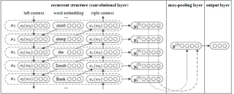
Figure 1. The structure of the cyclic convolution neural network.

determine which features play a key role in the emotional classification and capture the key components of the text. We combine the cyclic structure with the maximum pool layer, and give it the combined advantages of both the recurrent neural model and the convolution model. In addition, the time complexity of our model is and it has a linear relationship with the length of the text.

METHODOLOGY

In this paper, our task is to identify the polarity of documents, namely as positive and negative. We use two sets of criteria to evaluate sentiment analysis which include a 2-class and 5-class classification task. The 2-class includes positive and negative, and the 5-class contains positive, somewhat positive, neutral, somewhat negative and negative. The latter is a more fine-grained and thorough measurement. We will report accuracies and show analyses of the two metrics.

To capture the semantics of a document, we present a deep neural model. Figure 1 is our model’s network structure. The input of the network is the document D, which is the word w w₁, ₂, w_n sequence. The output of the network contains class

elements. We use p k D



| ,



to denote the probability of the document being class

k , where  represents the parameters in the network.

This figure is a partial example of the sentence “A sunset stroll along the South Bank affords an array of stunning vantage points”, and the subscript denotes the position of the corresponding word in the original sentence.

Pre-trained Word Vectors

Word embedding is a distributed representation of words. The distributed representation is applied to the input of the neural network. Traditional representations, such as thermal representations, lead to dimensionality. Recent studies have shown that neural networks can converge to a better local minimum with an appropriate unsupervised pre-training program.

In this work, we use the Skip-gram model to pre-embed the word. This model is the most advanced of all the NLP tasks. The Skip-gram model trains the embedding of words w w₁, ₂, w_T by maximizing the average log probability

1 , 0

1

log ( t j| t) c j c j

T

t

p w w

T

 

     

(1)

| | 1

exp( '( ) ( ))

( | )

exp( '( ) ( ))

b a

b a

k a

T

V _T

k

e w e w p w w

e w e w 





(2)

where V is the vocabulary of the unlabeled text. e w

 

_i is another embedded

i

Word Representation Learning

We combine a word and its context to express a word. We get more precise semantics through context. In our model, we use a regular structure to capture the background which is a bidirectional recurrent neural network.

We define cl(wi) as the left context of the word wi, cr(wi) as the right

context of the word wi. cl(wi ) and cr(wi) are the |C| of the dense vector of the

real value of the elements. The left side context cl(wi) of word wi is calculated

by formula (3), where e(wi−1) is the word embedding of word wi−1, which is a

dense vector with |e| real value elements. cl(wi-1) is the left side of the context

of the previous word wi−1. The left side of the first word in any document uses

the same shared parameter cl(w1). W(l) is the transformation of the hidden layer

(context) to the next layer of the hidden layer of the matrix. W(sl) is a matrix that is used to blend the semantics of the current word into the left context of the next word. f is a nonlinear activation function. cr(wi) is calculated in a

similar manner as shown in the formula (4). cr(wn) is for the right context of

the last word in the document.

( ) ( ( ) ( 1) ( ) ( 1))

l sl

l i l i i

c w  f w c w_ w e w_ (3)

c w_r( _i) f w c w( ( )r _r( _i1)w(sr)e w( _i1)) (4)

We can see from formulas (3) and (4) that the semantics of all the left and right contexts can be captured by the context vector. For example, in Figure 1, cl (w7)

encodes the semantics of the left-side context “stroll along the South” along with all texts in previous sentences, and cr (w7) encodes the semantics of the right-side

context “affords an ...”. Afterwards, we define the representation of word wi in

formula (5), which is the concatenation of the left-side context vector cl(wi), the

word embedding e(wi), and the right-side context vector cr(wi). In this way, with the

aid of this contextual information, our model is more powerful, more accurate, and more meaningful (i.e., it uses only part of the textual information) than the traditional neural model which uses only a fixed window of the neural model.

x_i [ (c w_{l i}); (e w_i);c w_r( _i)] (5)

Regular structures can take cl in all forward-scanned text, and get cr in all

backward-scanned text. Time complexity is O(n). We use xi to represent wi, and we

apply a linear transformation and hyperbolic tangent activation function to xi and

then input the result to the next layer.

y_i(2)tanh(W(2)x_ib(2)) (6)

yi(2) is a latent semantic vector, in which each semantic factor will be analyzed

Text Representation Learning

In our model, convolutional neural networks represent text. In convolutional neural networks, the recurrent structure we mentioned earlier is convoluted.

When all the words are evaluated, we apply a maximum pool level to it.

(3) (2)

1 max

n

i i

y y



 (7)

Here's the max function to smart elements. The kth element of y(3) is the maximum in the kth element of yi(2).

The pooling layer converts texts of various lengths into a fixed length vector. At the convergence layer, we can capture information throughout the document. There are other types of pool layers, such as the average pool layer [5]. We do not use average pooling here, because only a few words and their combinations are useful in capturing document meaning. The maximum layer attempts to find the most important underlying semantic elements in the document. The convergence layer uses the output of the regular structure as input. The convergence layer’s time complexity is O(n). The overall model is a cascade of regular structures and a maximum pond layer, so our model’s time complexity is still O(n).

Our model’s last part is an output layer. As in the traditional neural network, it is defined as:

y(4) W(4)y(3)b(4) (8)

At last, the softmax function is applied to y(4). It can output data into probabilities.

(4)

(4) 1

exp( )

exp( )

i

i n

k k

y p

y  



(9)

Training

We define the parameters of all we should train for θ.

 { ,E b(2),b(4), (c w_{l 1}),c w_r( _n),W(2),W(4),W( )l ,W( )r ,W( )sl ,W(sr)} (10)

In detail, the parameters are the word embeddings E∈ |e|×|V |, the bias vectors

b(2)∈ H,b(4)∈ O , the initial contexts cl(w1), cr(wn)∈ |c| and the transformation

matrixes W(2)∈ H×(|e|+2|c|), W(4)∈ O×H, W(l), W(r)∈ |c|×|c| , W(sl), W(sr)∈ |e|×|c| . Where |V| is the number of words in vocabulary, H is the hidden layer size and O is the number of document types.

The network training goal is to maximize the logarithm of θ like:

log p



_D| ,



D

class D

 



Where  is the training document set, classD is the correct class of document D.

We use a stochastic gradient descent to optimize training objectives. In each step, we randomly select an example (D, classD), and make a gradient step.

   log (p classD|D, )



  

 (12)

α is the learning rate.

We use one trick to train phrases, which is widely used when training neural networks with a stochastic gradient. We call initialization parameters from the uniform distribution of the neural network. Maximum or minimum size is equal to the square root of the "fan-in" [9]. The number is the network node of the previous layer in our model. The vector of the layer is divided by the "fan-in".

EXPERIMENTS

In this section, we will do some experiments to evaluate our model and show their analysis.

Dataset

We consider the corpus (Stanford Sentiment Treebank) of movie review excerpts from the rotten-tomatoes.com website originally collected and published by Pang and Lee (2005). The original dataset includes 10,662 sentences, half of which were considered positive and the other half negative. Each label is extracted from a longer movie review and reflects the writer’s overall intention for this review. The normalized, lowercase text is first used to recover, from the original website, the text with capitalization. Remaining HTML tags and sentences that are not in English are deleted. The Stanford Parser is used to parse all 10,662 sentences. [4] uses Amazon Mechanical Turk to label the resulting 215,154 phrases. It transfers the original 25 different values into 2 and 5 classes for classification. Our paper uses this dataset in our experiments. The dataset can be downloaded from http://nlp.stanford.edu/sentiment/.

As each phrase and sentence is labelled in the dataset, we will report the phrase and sentence prediction accuracies in experiments.

Experiments Settings

Hyper-parameters and Training. In our model, there are mainly three kinds of hyper-parameters: the number of hidden layer nodes n, the learning rate α for SGD and the coefficient λ for regularization items. We choose these hyper-parameters by obtaining the highest level of accuracy on a valid set. We select the number of hidden layer nodes among {50,100,150}, the regularization coefficients among {0.001,0.0001,0.00001} and the learning rate among {0.1,0.01,0.001}. On the movie review dataset for a 2-class classification, we select these hyper-parameters as n = 100, α = 0.01 and λ = 0.0001. As for a 5-class classification, we select them as n = 100, α= 0.01 and λ = 0.001.

Baseline Methods. We report the performance of the proposed models on sentiment classification tasks, and compare them with that of other competitor baseline systems. We show the related neural network baseline methods as follows: Recursive Neural Network, Matrix-Vector RNN, Recursive Neural Tensor Network, Convolutional Neural Network.

Results and Analysis

We include two types of analyses. The first type includes several large quantitative evaluations on the test set. The second type focuses on two linguistic phenomena that are important in sentiments. For all models, we use the dev set and cross-validate over regularization of the weights, word vector size, as well as learning rate and minibatch size for AdaGrad. We compare this with commonly used methods that use bag of words features with Naive Bayes and SVMs, as well as Naive Bayes with bag of bigram features. We abbreviate these with NB, SVM and biNB. We also compare with a model that averages neural word vectors and ignores word order (VecAvg).

TABLE I. ACCURACY FOR FINE GRAINED (5-CLASS) AND BINARY PREDICTIONS (2-CLASS) AT THE SENTENCE LEVEL (ROOT) AND FOR ALL NODES.

Model Fine-grained Positive/Negative

All Root All Root

NB 67.2 41.0 82.6 81.8

SVM 64.3 40.7 84.6 79.4

BiNB 71.0 41.9 82.7 83.1

VecAvg 73.3 32.7 85.1 80.1

RNN 79.0 43.2 86.1 82.4

MV-RNN 78.7 44.4 86.8 82.9

RNTN 80.7 45.7 87.6 85.4

CNN 79.3 45.5 86.8 81.9

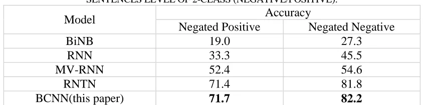
TABLE II. ACCURACY OF NEGATION DETECTION. NEGATED POSITIVE IS MEASURED AS CORRECT SENTIMENT INVERSIONS. NEGATED NEGATIVE IS MEASURED

AS INCREASES IN POSITIVE ACTIVATIONS. THIS EVALUATION IS CONDUCTED ON SENTENCES LEVEL OF 2-CLASS (NEGATIVE/POSITIVE).

Model Accuracy

Negated Positive Negated Negative

BiNB 19.0 27.3

RNN 33.3 45.5

MV-RNN 52.4 54.6

RNTN 71.4 81.8

[image:8.612.86.509.95.200.2]

BCNN(this paper) 71.7 82.2

Table I shows the experimental results of prediction accuracies. “All” represents the prediction of all nodes in sentences (phase level), while “root” represents the prediction of a sentence (sentence-level). In Fine-grained prediction, regardless of phrase and sentence level, RCNN (our proposed model) outperforms all the baseline methods including RNN, MV-RNN, RNTN and CNN, which indicates that RCNN can combine the advantages of RNN and CNN. In Positive/Negative prediction, RCNN also achieves state-of-the-art performance on sentence level. Although RNTN obtains better accuracy than RCNN a little on phrase level, the RNTN has numerous parameters and a high cost.

We investigate two types of negation. For each type, we use a separate dataset for evaluation. The first is Negating Positive Sentences. It contains positive sentences and their negation. In this set, the negation changes the overall sentiment of a sentence from positive to negative. The second is Negating Negative Sentences. It contains negative sentences and their negation. When negative sentences are negated, the sentiment treebank shows that overall sentiment should become less negative, but not necessarily positive. For instance, “The movie was terrible” is negative but “The movie was not terrible” says only that it was less bad than a terrible one, not that it was good. Hence, we compute accuracy in terms of correct sentiment reversal from positive to negative, and evaluate accuracy in terms of how often each model was able to increase non-negative activation in the sentiment of the sentence. Table II shows the accuracy of the two types of negation in the dataset of several models. From Table II, we can see that our approach outperforms all the baseline systems on both types of negation. It indicates that our model can capture linguistic sentiment details.

CONCLUSIONS AND FUTURE WORK

In the future, the work we may explore includes 1) extending the RCNN to other natural language processing tasks including relation extraction, sentence classification and sentence matching; 2) exploring the algorithm to reduce the number of parameters because our model requires numerous parameters for large datasets.

REFERENCES

1. Pang B and Lee L. 2008. “Sentiment Analysis and Opinion Mining”, Foundations and trends in information retrieval, vol. 2, no. 1-2, pp. 1-135.

2. R Socher, EH Huang, J Pennington, AY Ng and CD Manning. 2011. “Dynamic Pooling and Unfolding Recursive Autoencoders for Paraphrase Detection”, Advances in Neural Information Processing Systems., vol. 24, pp. 801-809.

3. R Socher, J Pennington, EH Huang, AY Ng and CD Manning. 2011. “Semi-Supervised Recursive Autoencoders for Predicting Sentiment Distributions”, Proceedings of the Conference on Empirical Methods in Natural Language Processing, Edinburgh, United Kingdom, July 27-31, 2011.

4. Richard Socher, Alex Perelygin, Jean Y. Wu, Jason Chuang, Christopher D. Manning, Andrew Y. Ng and Christopher Potts. 2013. “Recursive Deep Models for Semantic Compositionality Over a Sentiment Treebank”, Proceedings of the conference on empirical methods in natural language processing, Seattle, USA, October 18-21, 2013.

5. Ronan Collobert, Jason Weston, Léon Bottou, Michael Karlen, Koray Kavukcuoglu and Pavel Kuksa. 2011. “Natural Language Processing (Almost) from Scratch”, The Journal of Machine Learning Research, Vol.12, pp. 2493-2537.

6. N Kalchbrenner and P Blunsom. 2013. “Recurrent Convolutional Neural Networks for Discourse Compositionality”, Proceedings of the Workshop on Continuous Vector Space Models and their Compositionality - Association for Computational Linguistics, Sofia, Bulgaria, August 9, 2013. 7. Mathieu Cliche. 2017. “Task 4: Twitter Sentiment Analysis with CNNs and LSTMs”, Proceedings

of the 11th International Workshop on Semantic Evaluation, Vancouver, Canada, August, 2017. 8. S Lai, L Xu, K Liu and J Zhao. 2015. “Recurrent convolutional neural networks for text

classification”, Proceedings of the Twenty-Ninth AAAI Conference on Artificial Intelligence, Austin Texas, USA, January 25-30, 2015.

9. Polanyi L and Zaenen A. 2006. “Contextual Valence Shifters”, Information Retrieval., vol. 20, pp. 1-10.

10. Mikolov T A. 2012. “Statistical Language Models Based on Neural Networks”, Presentation at Google, CA, USA, April 2, 2012.