High Order Compact Scheme and the Moving Mesh Method for Helmholtz Equation with Variable Wave Numbers

2016 International Conference on Mathematical, Computational and Statistical Sciences and Engineering (MCSSE 2016) ISBN: 978-1-60595-396-0

High Order Compact Scheme and the Moving Mesh Method for

Helmholtz Equation with Variable Wave Numbers

Fu-jun CAO

1,*

, Dong-fang YUAN

1

and Yong-bin GE

2

1_{School of Science, Inner Mongolia University of Science and Technology, Baotou, Inner Mongolia}

014010, China

2

Institute of Applied Mathematics and Mechanics, Ningxia University, Yinchuan, Ningxia 750021, China

*Corresponding author

Keywords: High order compact scheme, Helmholtz equation, Moving mesh method, Non-uniform mesh.

Abstract. High order compact scheme has extensively been used for solving the Helmholtz equation on uniform mesh. Although uniform spacing is computationally advantageous for isotropic problems, the non-uniform mesh will be superior to the problems with the anisotropic properties or boundary layers. In this paper, we proposed a compact scheme on nonuniform mesh which has at least third order accuracy for the 2D Helmholtz equation with variable wave number. A novel adaptive mesh algorithm is also presented to generate the orthogonal nonuniform mesh. The 2D Helmholtz equation is solved by combining the HOC scheme on nonuniform mesh with the moving mesh method. The multigrid method is used to solve the discrete algebraic system. Numerical experiments are executed to verify the accuracy and efficiency of the presented method.

Introduction

The Helmholtz equation governs wave propagation and scattering phenomena arising in acoustic problems in many areas, e.g., in aeronautics, marine technology, geophysics, and optical problems. Much effort has been invested and a widely range of numerical methods has been proposed for solving the Helmholtz equation, such as, the finite volume method, finite element method, finite difference method and spectral element method. The compact finite difference scheme has been extensively studied for solving the Helmholtz equation on the behalf of high order accuracy on small stencils. Starting from the noticeable work [1], a family of high-order compact schemes are derived for variety of Helmholtz equations based on the differencing of governing equation to eliminate higher order derivatives in the discretization error, such as, the compact finite difference scheme for one dimension problems[2], the compact fourth order accuracy finite difference approximation for two and three dimension problems on the Cartesian coordinate [1,3] and polar coordinates[4,5]. Other papers have extended the HOC scheme to Helmholtz equation with non-homogeneous materials [6], with nonstandard boundary conditions [7] and with singular solutions[8]. Recently, more accurate compact sixth order methods are considered for solving the Helmholtz equation with a constant wave number [9, 10,11] and a variable wave number [12].

The adaptive mesh method has been widely researched and applied in solving the partial differential equation with large solution variations or boundary layers. Tang and Tang[20] develop efficient moving mesh algorithms for one- and two-dimensional hyperbolic systems of conservation laws by using rezoning moving mesh methods where physical partial differential equations(PDEs) were integrated on a uniform mesh over a time step and conservative interpolation was used to transfer solutions from the old mesh to the new mesh. In one dimension, it is show that the underlying numerical approximation obtained in the mesh-redistribution part satisfies the desired total variation diminishing (TVD) property. However, the finite volume mesh produced by the algorithm for 2D problems lose of orthogonality and can’t be directly extended to finite difference scheme.

In this paper, we derive a compact difference scheme on nonuniform mesh for the two dimensional Helmholtz equation with variable wave number. The presented scheme is of at least three order accuracy assuming the variables u, k and the source term f are sufficiently smooth. A novel adaptive mesh algorithm is proposed to generate orthogonal nonuniform computational mesh for 2D rectangular domain based on the 1D algorithm by [16]. Moreover, in order to accelerate the solving efficiency, the multigrid method in [14] is applied to solve the discrete linear system.

This paper is organized as follows. In Section 2, we introduce the compact difference scheme on nonuniform gird for Helmholtz equation with variable wave number. In Section 3, an adaptive mesh algorithm is provided to generate the orthogonal nonuniform mesh for the two dimensional domain. The numerical results are executed in Section 4 to verify the accuracy and efficiency of the present method. The conclusion is summarized in Section 5.

The Compact Scheme on Nonuniform Mesh

Consider the two-dimensional Helmholtz equation with variable wave number

2

( , ) ( , ), ( , )

xx yy

u u k x y u f x y x y 

, (1) where  [ , ] [ , ]a b  c d and ( , )k x y is the function of wave number. The variable u _{and the source}

function ( , )f x y are assumed to be differentially smooth.

First, we discrete the computational domain in each direction by sub-intervals with arbitrary steps donated as xand y, i.e.,

1 0

1 0

{ } { | [ , ], , 0,1, , 1, , },

{ } { | [ , ], , 0,1, , 1, , },

x

y

i i i i x N

j j j j y N

x x x a b x x i N x a x b

y y y c d y y j N y c y d





      

      

where N_x and N_y are grid number at xand y direction, respectively.

Denote h_x  (b a) /N_x, the forward and backward step sizes are given as

1 , 1 , 1 1.

fx i i fx x bx i i bx x x

h x_  x  h h  x x_  h  i N 

Similarly, let h_y (dc) /N_y, and

1 , 1 , 1 1.

fy j j fy y by j j by y y

h  y _ y  h h  y y _  h  j N 

For the sake of expression simplicity, let _x   _{fx bx}, _x _fx _bx, _x _fx_bx. Similarly,

,

y fy by

   y fy by, y fyby. Using the Taylor series expansion, and eliminating higher order derivatives in the discretization error by the differencing of governing equation, the compact nine point difference scheme on nonuniform grids for 2D Helmholtz equation can be written as

2 2

8

0 0 0 0

0 1 1 2 2 2 2

0

i i

f f f f

A f H L H L

x y x y



   

    

   



2 2 2

0 0 2 2 0 1 0 1 0 0 1 0 1

2 2

2 2 2 2 2 2

1 2 1 2 0 2 0 2 0 2 2 2 2

1 1

2( ) 2 ( )

2 2 2 2 4( )

2 ( ) ,

y y x x

x y

x x y y x x x y y y

y x x x y y

x y

y y y x x y x x x y y y x x y y x y x y

A k k H k L k k H k L

h h h h

k H k L H L

H L k H k L k

h h h h h h h h

                                                2

1 2 2

2 1 0 2

1 2 0 1 2 2 2 2 2

4( )

2 1 1 2 2 2

( ) ( ) + y y bx,

bx x bx x bx bx bx

x x x x x x x x x x x x x y y x x x y y x x x x y x y x y

L k H H L

H

A k H

h h h h h h h h h h h

                                    2

0 2 2 2

2 1 1

2 2 0 1 2 2 2 2 2

2 ₁ 2 _{2 1} 2 4( )

( ) ( )+ ,

by y fy by x y by by x by

y y y y y y y y y y y x x x x y y y y y y y y x y x y x y

k L H L

H L

A k L

h h h h h h h h h h h

         

                 



      

2

1 2 2 2

2 1

3 2 1 0 2 2 2 2 2

2 _{1 2 1} 2 2 4( )

( ) ( )+ ,

fx x fx x fx fx y fx y fx

x x x x x x x x y y y x x x x x x x x y y x x x x y x y x y

L k H H L

H

A H k

h h h h h h h h h h h

         

                  



      

2

0 2 2 2

2 1 1

4 2 0 1 2 2 2 2 2

2 1 2 1 2 2 4( )

( )+ ( ) ,

fy y fy y fy fy fy x x fy

y y y y y y y y x x y y y y y y y y y y y x x x y x y x y

k L H H L

L

A k L

h h h h h h h h h h h

       _  

                 



      

1 ₁ 2 2

5 2 2 2 2 1

2 2 4( )

, ,

3

by _bx bx by _{x x}

y y x x y x x y y x x y x y x y

H L H L h

A H

h h h h h h

    

         



   

2 2

1 1 2 2

6 2 2 2 2 2

2 2 4( ) ( 3 )

,

12

fx by by fx x x x

x y x y x y x y x y x y x y x y

L H H L h

A H

h h h h h h

     

         

 

    ，

1 2 2

1

7 2 2 2 2 1

2 4( )

2

, ,

3

fy fy bx y y

bx

x y x y x y x y x y x y x y x y

H H L h

L

A L

h h h h h h

                     2 2

1 1 2 2

8 2 2 2 2 2

2 2 4( ) ( 3 )

. 12

fy fx fx fy y y y

y y x x y x x y y x x y x y x y

H L H L h

A L

h h h h h h

     

         

 

    ， 

The scheme (2) is of at least three order accuracy on non-uniform mesh. Once _fx  _bx, _fy _by the step sizes on the both x _and y directions are equal, then the mesh is uniform and the scheme (2) has fourth order accuracy. For more details about the derivation process, one can refer to [13, 14].

Moving Mesh Algorithm

Although plenty of moving mesh method are presented for 2D problems, most of them aim at the finite volume method which neglect the orthogonality of mesh and unable to be directly used for finite difference scheme. In this section, the adaptive mesh algorithm for 2D rectangular domain is proposed to generate orthogonal computational mesh. The dimension split idea is applied to fulfill this aim which simplifies the implementation process and improves the efficiency of the algorithm. The presented algorithm is suitable for the problems in which the boundary layers are parallel to the coordinate axis.

Locating the Boundary Layer

The uniform mesh for the 2D computational domain is used as the initial mesh and denoted as [0]

( , )

coord i j , i.e., coord[0]( , )i j {( ( ), ( )) |x i y j i0,1, ,Nx,j0,1, ,Ny}. Given a well posed problem with boundary layers, we solve the problem on the uniform mesh coord[0] _{and get a}

estimated result as the initial value denoted as [0]

u _{. The adaptive mesh method will be executed based}

on the initial mesh coord[0] _{and the initial value} u[0].

1 [0]

1/2, 0

( ) | |, 0,1, , x

N r

i j y

i

sg j u j N



 





  ， [0] [0] [0] [0] [0] 1/ 2, ( 1 ) / ( 1 )

i j i i i i

u u u x x

    .

Similarly, the summation of gradient at i th column can be obtained and denoted as

{sg i ic( ), 0,1, ,N_x}

. Let imax be the index of {sg i ic( ), 0,1, ,Nx} which has the maximum

value, i.e., imax{ | maxi sg i ic( ), 0,1, ,N_x}_{. It means that the solution at the} imax-th row varies most intensely. Similarly, we can define the jmax{ | maxj sgr( ),j j0,1, ,Ny}. Denote the

maximum cell gradient on imax row and imax column as maxr and maxc, respectively.

1/ 2, , 1/ 2

max | |, max | | .

r c

i jmax imax j

max  u_ max  u _

Define layy maxr /sgr(jmax), layx maxc/sg imaxc( ). The values of layy _and layx _{will be}

used to detect the large solution variations. When layy _and layx _{are large, then the solution at these}

cells vary intensely. In order to get more accurate numerical solutions, it need to distribute more grid points in this region. Given a threshold parameter  _{, there are four cases should be considered.}

Case 1. {layx ,layy}_{, it means that the solutions on the both directions are relatively smooth} and uniform mesh is enough and the adaptive mesh is unnecessary.

Case 2. {layx,layy }_{, it means that there is a boundary layer parallel to} y axis, the adaptive mesh algorithm should be performed along this direction.

Case 3. _{layx ,layy }, it means the boundary layer is parallel to x axis and the grid points along this direction should be adjusted and clustered to the large gradients region.

Case 4. {layx ,layy }. In this case, there are two boundary layers on each directions and they intersect each other. In practice, the threshold parameter  is chosen to be 0.3.

Moving Mesh by Iteration

To begin with, the idea of 1D adaptive algorithm is described. Based on the standard equidistribution principle, the mesh generation equation for one-dimensional is

(x_{ }) 0,

where  is the monitor function. Solving the above equation by Gauss-Seidel-type iteration proposed in [20] with an uniform mesh x[0] _{and initial value} u[0], a map between the physical domain

p

 and the logical domain _c can be computed.

[ ] [ ] [ 1] [ ] [ 1] [ 1]

1 1 1 1

2 2

( )( _{j j} ) ( )( _{j j} ) 0,

j j

u x x u x x

    

 

     

where  is the iteration number, x[ ]j 1 

 is the coordinate of the (j1)-th point at -th iteration.Repeat the above process for a fixed number of iterations or until [ 1] [ ]

1 x x 

‖ ‖ . The new mesh based on

the initial mesh x[0] and value u[0] is obtained and denoted as x. For more details about the 1D adaptive mesh algorithm, one can refer to [16].

None lose of generality, as for 2D problem, we consider the Case 4. There are boundary layers exist in both directions. The alternating direction 1D adaptive mesh algorithm can be applied separately to generate the nonuniform mesh on x and y direction. Let {x_r[0][ ]i x[0]( ),i

[0] [0]

[ ] ( , ), 0,1, , }

x x

u i u i jmax i N and [0] [0]

{y_r [ ]j  y ( ),j u[0]_y [ ]i u[0](imax j, ), j0,1, ,N_y} . Given{x[0]_r ,u[0]_x } and {y[0]_c ,u[0]_y } as initial data, the 1D adaptive mesh algorithm will be perform for

as coord[1]( , )i j {(x[1]( ),i y[1]( )),j i0,1, ,Nx, j0,1, ,Ny} _{. After obtaining the new value} [1]

coord , we need to update the solution from [0]

u to [1]

u by the bilinear interpolation

[0] [0] [0] [0]

[1] [0] [1] [0] [1] [0]

[0] [0] [0] [0]

[1] [0] [0] [1] [0] [0]

( 1, ) ( , ) ( , 1) ( , )

( , ) ( , ) ( ( ) ( )) ( ( ) ( )),

( 1) ( ) ( 1) ( )

( ) ( ( ), ( 1)), ( ) ( ( ), ( 1)).

u i j u i j u i j u i j

u i j u i j x i x i y j y j

x i x i y j y j

if x i x i x i y j y j y j

   

    

   

   

Repeat the above processes and until coord[ 1] coord[ ] 2

 _  _

, the new mesh coord _{can be}

generated. Similarly, as for Case 2 and Case 3, the boundary layers are exists either in xor y direction. Therefore, the 1D adaptive mesh algorithm is performed for the solution intensely varied direction, and the uniform mesh is kept for the smooth solution direction.

Numerical Example

In this section, the numerical experiments are executed to verify the effectiveness and accuracy of the present method. The numerical results from the HOC scheme on nonuniform mesh and adaptive mesh method are compared with those on uniform and nonuniform mesh by the grid stretching function [13,14].

Example 1 Consider the problem which has two boundary layer at x1 _and y1_{. The}

0

( , ) 1 ( ), ( ) cos( ).

k x y k m x m x  x The analytical solution is

( 1) ( 1) 2

(1 )(1 )

( , ) .

(1 )

x y

e e

u x y

e

 



 



 





The source term can be calculated by the analytical solution. The parameters k₀ 10,0.3and

0 0.2k

[image:5.595.67.525.455.553.2]

  are used in computation. The monitor function used for this problem is 2

1 0.15 |u_|

  .

In order to get the nonuniform mesh, the grid stretching parameter x y 0.6and xy 0.9 are

used for 2

10

  _and 3

10

  , respectively.

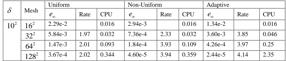
Table 1. The comparison of maximum error, CPU time and Rate.

 Mesh

Uniform Non-Uniform Adaptive

e_ Rate CPU e_ Rate CPU e_ Rate CPU

2

10 162 2.29e-2 0.016 2.94e-3 0.016 1.34e-2 0.016

2

32 5.84e-3 1.97 0.032 7.36e-4 2.33 0.032 3.60e-3 3.85 0.046

2

64 1.47e-3 2.01 0.093 1.84e-4 3.93 0.109 4.26e-4 3.97 0.25

2

128 3.67e-4 2.02 0.344 4.60e-5 3.94 0.359 2.44e-5 4.14 2.35

Table 1 compares the maximum error, CPU time and convergence rate under three kinds of meshes. when  102, the accuracy and convergence rate on three kinds of meshes are acceptable. The maximum errors on nonuniform mesh and adaptive mesh are much lower than that by uniform mesh. When  103 the solution become steep in the boundary layers, the accuracy of numerical solution on uniform mesh loss. The accuracy of the solution on other two kinds of meshes still keeps.

(a) (b)

[image:6.595.110.490.69.488.2]

(c) (d)

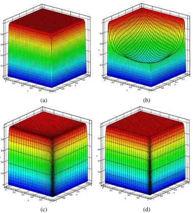
Figure 1. The plot of exact solution(a), numerical solution on uniform mesh(b), nonuniform mesh(c) and adaptive mesh(d)

with grids number N_x 33,N_y 33 for 3

10

  _.

Figure 2. The comparison of exact solution with numerical solution on uniform mesh(a), nonuniform mesh(b) and adaptive

mesh(c) at line y0.9 with grids number _{65, 65}

x y

[image:6.595.64.534.538.708.2]

Summary

We present a HOC scheme on nonuniform mesh for 2D Helmholtz equation with variable wave number. This scheme is of at least third order accuracy on nonuniform mesh and fourth order on uniform mesh. A novel adaptive mesh algorithm is proposed to generate orthogonal nonuniform mesh for 2D domain which cluster the grid points to the region of large variation gradients according to the solution structure. Combining the HOC scheme on nonuniform mesh with the adaptive mesh method, the 2D Helmholtz equation with boundary layers are solved to test the validity and effectiveness of the presented method. Numerical results show that the presented method is supervisor to the HOC scheme on uniform. Besides, it is effective to be implemented and be able to improve the accuracy of numerical solution.

Acknowledgment

This work was supported by the Foundation of National Nature Science Foundation of China (11361045), and the Foundation of Science of Inner Mongolia University of Science and Technology (2014QDL004).

References

[1] I. Singer, E. Turkel, High-order finite difference method for the helmholtz equation, Comput. Methods Appl. Mech. Eng., 163 (1998) 343-358.

[2] K. Wang, Y.S. Wong, Pollution-free finite difference schemes for non-homogeneous Helmholtz equation, Int. J. Numer. Anal. Model., 4(11) (2014) 787-815.

[3] Y. Fu. Compact fourth-order finite difference schemes for Helmholtz equation with high wave numbers. J. Comput. Math., 26(1) (2008).

[4] S. Britt , S. Tsynkov ,E. Turkel . A compact fourth order scheme for the Helmholtz equation in polar coordinates. J. Sci. Comput., 45(1-3) (2010) 26-47.

[5] K. Wang, Y. S. Wong, J. Deng. Efficient and Accurate Numerical Solutions for Helmholtz Equation in Polar and Spherical Coordinates, Commun. Comput. Phys., 17(03) (2015) 779-807.

[6] Britt, S., Tsynkov, E. Turkel. Numerical simulation of time-harmonic waves in inhomogeneous media using compact high order schemes. Commun. Comput. Phys., 9(3) (2011) 520-541.

[7] Britt, S., Tsynkov, E. Turkel. A high-order numerical method for the Helmholtz equation with nonstandard boundary conditions. SIAM J. Sci. Comput., 35(5) (2013) A2255-A2292.

[8] S. Britt, S. Petropavlovsky, S. Tsynkov, et al. Computation of singular solutions to the Helmholtz equation with high order accuracy. Appl. Numer. Math., 93 (2015) 215-241.

[9] S.O. Settle, C.C. Douglas, I. Kim, D. Sheen, On the derivation of highest-order compact finite difference schemes for the one- and two-dimensional Poisson equation with Dirichlet boundary conditions, SIAM J. Numer. Anal., submitted for publication.

[10] M. Nabavi, M. H. K. Siddiqui ,J. Dargahi. A new 9-point sixth-order accurate compact finite-difference method for the Helmholtz equation. J. Sound Vibr., 307(3) (2007) 972-982.

[11] G. Sutmann, Compact finite difference schemes of sixth order for the Helmholtz equation, J. Comput. Appl. Math., 203(1) (2007) 15-31.

[12] E. Turkel, D. Gordon, R. Gordon , S. Tsynkov, Compact 2D and 3D sixth order schemes for the Helmholtz equation with variable wave number, J. Comput. Phys., 232 (2013) 272-287.

[14] Y. B. Ge, F. J. Cao, Multigrid method based on the transformation-free HOC scheme on nonuniform grids for 2D convection diffusion problems, J. Comput. Phys., 230 (2011) 4051-4070.

[15] Y. B. Ge, F. J. Cao, J. Zhang.A transformation-free HOC scheme and multigrid method for solving the 3D Poisson equation on nonuniform grids. J. Comput. Phys., 234 (2013) 199-216.