Temporal Aggregation for ARMA Model in an Application Perspective

2017 2nd International Conference on Computational Modeling, Simulation and Applied Mathematics (CMSAM 2017) ISBN: 978-1-60595-499-8

Temporal Aggregation for ARMA Model in an Application Perspective

Ze-hui JIN, Ying-ying HU, Jia-liang HUA and Zeng-min WANG

Beijing University of Posts and Telecommunications, China

*Corresponding author

Keywords: ARMA, Temporal aggregation, Monte Carlo, Model optimization.

Abstract. This article perfects ARMA model explanations and discusses regularity results of ARMA model in temporal aggregation. Monte Carlo simulation has been applied to verify accuracy of the theory. And we also put forward possible model applications, that is, integrating shocks to better prediction model in financial markets.

Introduction

Shocks are frequently witnessed by the financial market, to efficiently and timely integrate these unexpected fluctuations into the forecasting model will benefit players for huge profit or less loss. People modify their models according to a certain time unit—for example, players will update their stock forecasting model after every trading day. Suppose that, if the shock happens at the mid of the day, then players have to suffer that afternoon since they couldn’t integrate this shock into the model immediately so they are not able to make moves according to quantitative analysis but intuitions.

Temporal aggregation accounts for this phenomenon, that is, the frequency of data collection is lower than the frequency at which data are generated, thus part of items in the original random process 𝑥 = {𝑥_𝑡}_𝑡=0∞ are missing, only items after aggregation 𝑋 = {𝑋_𝜏}_𝜏=0∞ can be observed, where 𝑡 is the original frequency and 𝜏 is the after-aggregation frequency, 𝑋 is a specific function of 𝑥 determined by the aggregation scheme (Marcellino, 1999). In the above case, trading data are generated at every minute while people only gather them at every day. Temporal aggregation model is a great method to fix this problem by ‘transferring’ time unit to integrate every single hour data or even every minute data (not realistic though) into the daily model for optimization. So once data is available, players could improve their model to better its forecasting ability.

The study of temporal aggregation was started by Amemiya and Wu (1972), who first proposed the view that the structure of AR model remains unchanged after temporal aggregation. Brewer (1973) derived ARMAX model with exogenous variable x to further improve theories. William (1978) stated that seasonality has to be considered when the temporal aggregation frequency is greater than the nature frequency of data. Weiss (1994) discussed flow and stock variables separately for ARIMA models. Seater (1995) explored the periodic variation of the time series before and after temporal aggregation, and found that the monthly and quarterly data have lower frequency fluctuations and the annual data completely loses the periodic fluctuation; in other words, there exists information loss. The discussion paper of Andrea Silvestrini and David Veredas in 2005 reviewed temporal aggregation of ARIMA, ARMA-GARCH, VARMA and GARCH models, and it was published in 2008 in an official version. Temporal aggregation has been discussed for over 30 years, but most attention has been focused on the theoretical level, little has been done to practical applications.

ARMA Model

Model Derivation

In this section, we will focus on the stock case 𝑦𝑡∗ = 𝑦𝑘𝑡, where k is the aggregation frequency. We

also mention flow case at the end of this section. The ARMA model is defined as

𝜙(𝐿) ⋅ 𝑦_𝑡= 𝜃(𝐿) ⋅ 𝜖_𝑡. (1) Where 𝑡 = 0,1,2, ⋯, 𝜙(𝐿) and 𝜃(𝐿) are both polynomials of lag operator 𝐿, 𝜙(𝐿) = 1 − 𝜙1𝐿 − ⋯ − 𝜙𝑝𝐿𝑝, 𝜃(𝐿) = 1 + 𝜃1𝐿 + ⋯ + 𝜃𝑞𝐿𝑞, and 𝜖𝑡 ∼ 𝑁(0, 𝜎𝜖2). We assume 𝜙(𝐿) and 𝜃(𝐿)

have distinct roots that lie outside the unit circle. Let 𝛿𝑗(𝑗 = 1,2, … 𝑝) be the inverted roots of 𝜙(𝐿) which are inside the unit circle, then 𝜙(𝐿) can be expressed as ∏𝑝_𝑗=1(1 − 𝛿_𝑗𝐿).

We define the model after temporal aggregation as

𝛽(𝐵) ⋅ 𝑦_𝑇∗ = 𝜂(𝐵) ⋅ 𝜖_𝑇∗. (2) Where 𝑇 = 0, 𝑘, 2𝑘, ⋯, 𝛽(𝐵) and 𝜂(𝐵) are both polynomials of lag operator 𝐵 = 𝐿𝑘_, 𝛽(𝐵) = 1 − 𝛽₁𝐵 − ⋯ − 𝛽_𝑐𝐵𝑐_{, 𝜂(𝐵) = 1 + 𝜂}

1𝐵 + ⋯ + 𝜂𝑟𝐵𝑟, 𝑦𝑇∗ is the dependent variable after

aggregation and 𝜖_𝑇∗ is the white noise after aggregation.

In this case, 𝜙(𝐿) ⋅ 𝑦𝑡 = 𝜃(𝐿) ⋅ 𝜖𝑡 model represents model for data gathered per minute, the

time unit is short, the information amount is great but the fluctuation is too huge for prediction. While 𝛽(𝐵) ⋅ 𝑦_𝑇∗ _{= 𝜂(𝐵) ⋅ 𝜖}

𝑇

∗ _{model represents daily model which is perfect for reference.}

We use polynomial 𝑇(𝐿) = 1 + 𝑡₁𝐿 + 𝑡₂𝐿2+ ⋯ + 𝑡_ℎ𝐿ℎ to connect these two models, so that once 𝜙(𝐿) ⋅ 𝑦_𝑡 = 𝜃(𝐿) ⋅ 𝜖_𝑡 is updated, 𝛽(𝐵) ⋅ 𝑦_𝑇∗ _{= 𝜂(𝐵) ⋅ 𝜖}

𝑇

∗ _{can be adjusted as well.}

𝑇(𝐿) ⋅ 𝜙(𝐿) ⋅ 𝑦_𝑡 = 𝛽(𝐵) ⋅ 𝑦_𝑇∗_{. (3)}

𝑇(𝐿) ⋅ 𝜃(𝐿) ⋅ 𝜖𝑡 = 𝜂(𝐵) ⋅ 𝜖𝑇∗. (4)

According to the first formula above, we have

(1 + 𝑡₁𝐿 + 𝑡₂𝐿2_{+ ⋯ + 𝑡}

ℎ𝐿ℎ) ⋅ (1 − 𝜙1𝐿 − ⋯ − 𝜙𝑝𝐿𝑝) ⋅ 𝑦𝑡

= (1 + 𝛽₁𝐵 + 𝛽₂𝐵2_{+ ⋯ + 𝛽}

𝑐𝐵𝑐) ⋅ 𝑦𝑇∗. (5)

Brewer (1973) indicated the matrix form of 𝑇(𝐿), thus 𝑇(𝐿) ⋅ 𝜙(𝐿) = 𝛽(𝐵) can be expressed as

[

1 0 ⋯ 0

𝑡₁ 1 ⋯ 0

𝑡₂ 𝑡₁ 1 0

⋮ ⋮ ⋮ ⋮

𝑡_𝑝 𝑡_𝑝−1 ⋯ 1

⋮ ⋮ ⋮ ⋮

𝑡ℎ 𝑡ℎ−1 ⋯ 𝑡ℎ−𝑝

0 𝑡_ℎ ⋯ ⋯

0 0 𝑡_ℎ ⋯

0 0 0 𝑡_ℎ ]

⋅ [ 1 −𝜙₁

⋮ −𝜙_𝑝

] =

[ 1 0 ⋮ 𝛽₁

0 ⋮ 𝛽₂

0 ⋮ 𝛽_𝑐]

. (6)

Note that

1) Matrix 𝑇(𝐿) is comprised of coefficients of lag operator 𝐿, the first line represents 𝐿0_{, the}

second line is 𝑡1𝐿1+ 𝐿0, the third line is 𝑡2𝐿2+ 𝑡1𝐿0+ 𝐿0, and so forth. Because the highest

power of 𝑇(𝐿) is ℎ, so the ℎ + 1 line represents 𝑡_ℎ𝐿ℎ_{+ 𝑡}

ℎ−1𝐿ℎ−1… + 𝑡ℎ−𝑝𝐿ℎ−𝑝. And

(−𝜙_𝑖) is the coefficient of 𝐿𝑖 in 𝜙(𝐿). Only those 𝐿𝑖𝑘(𝑖 = 0,1,2 … )̇ have non-zero coefficients in 𝛽(𝐵).

𝛽(𝐵) is 1. Similarly, the last item of 𝑇(𝐿), 𝐿ℎ, has non-zero coefficient 𝑡ℎ, the last item of 𝜙(𝐿), 𝐿𝑝, has non-zero coefficient (−𝜙𝑝), so the last item of 𝛽(𝐵), 𝐿ℎ+𝑝, has non-zero

coefficient 𝛽𝑐.

3) Matrix 𝑇(𝐿) is (𝑝 + ℎ + 1) × (𝑝 + 1), 𝜙(𝐿) is (𝑝 + 1) × 1, 𝛽(𝐵) is (1 + 𝑐𝑘) × 1, where 𝑝 is known, ℎ and 𝑐 can be calculated by constriction equations. From the view of matrix multiplication, number of rows of 𝑇(𝐿) must be equal with that of 𝛽(𝐵), thus the first equation is 𝑝 + ℎ + 1 = 1 + 𝑐𝑘. From the view of matrix solutions, the number of unknown coefficients ℎ in 𝑇(𝐿) must match with 𝑐(𝑘 − 1) conditions in 𝛽(𝐵), thus the second equation is ℎ = 𝑐(𝑘 − 1). From these two equations we can yield that 𝑐 = 𝑝,

ℎ = 𝑝(𝑘 − 1).

𝑇(𝐿) can be calculated through the above matrix. In this case, we give the qualifying 𝑇(𝐿)

expression without proof

𝑇(𝐿) = ∏ 1−𝛿𝑗

𝑘_𝐿𝑘

1−𝛿𝑗𝐿

𝑝

𝑗=1 = ∏ (

𝑝

𝑗=1 ∑𝑘−1𝑖=0 𝛿𝑗𝑖𝐿𝑖). (7)

Since the polynomial T (L) is given based on the AR(𝑃) model, so the aggregation of AR(𝑃)

model is easy to operate.

𝑇(𝐿) ⋅ 𝜙(𝐿) ⋅ 𝑦_𝑡 = ∏𝑝_𝑗=1[1−𝛿𝑗

𝑘_𝐿𝑘

1−𝛿𝑗𝐿] ⋅ ∏ (

𝑝

𝑗=1 1 − 𝛿𝑗𝐿) ⋅ 𝑦𝑡

= ∏𝑝_𝑗=1(1 − 𝛿_𝑗𝑘𝐿𝑘) ⋅ 𝑦_𝑡 = ∏𝑝_𝑗=1(1 − 𝛿_𝑗𝑘𝐵) ⋅ 𝑦_𝑇∗ _.

(8)

By contrast, the operation of MA(q) is quite tough, which has to be solved by an equation system

𝑇(𝐿) ⋅ 𝜃(𝐿) ⋅ 𝜖𝑡 = ∏𝑝𝑗=1[ 1−𝛿_𝑗𝑘𝐿𝑘

1−𝛿𝑗𝐿] ⋅ (∑ 𝜃𝑑

𝑞

𝑑=0 𝐿𝑑) ⋅ 𝜖𝑡

= ∏𝑝_𝑗=1(∑𝑘−1_𝑖=0 𝛿_𝑗𝑖𝐿𝑖) ⋅ (∑𝑞𝑑=0𝜃𝑑𝐿𝑑) ⋅ 𝜖𝑡 = ∏𝑝_𝑗=1(∑𝑘−1_𝑖=0 𝛿_𝑗𝑖𝐿𝑖_{)(∑ 𝜃}

𝑑 𝑞

𝑑=0 𝐵) ⋅ ϵT.

(9)

Where 𝜃₀ = 1, the order of 𝜖_𝑇 is 𝑟 = 𝑝(𝑘 − 1) + 𝑞, the order of 𝜖_𝑇∗ _{is 𝑟 = ⌊}𝑝(𝑘−1)+𝑞 𝑘 ⌋, and ⌊𝑏⌋ indicates the integer part of a real number b.

𝑇(𝐿) ⋅ 𝜃(𝐿) ⋅ 𝜖_𝑡 ≡ 𝜂(𝐵) ⋅ 𝜖_𝑇∗_{. (10)}

The coefficients of 𝜂(𝐵) are solved by equalizing the variance and the auto-covariance of R.H.S and L.H.S of the above equation. Since 𝜂(𝐵) has the highest r order, so it has a total of r auto-covariances. Hence it becomes a problem of solving a system of equations with (r + 1) unknowns and (r + 1) nonlinear equations.

Let 𝐺_𝑡= 𝑇(𝐿) ⋅ 𝜃(𝐿) ⋅ 𝜖_𝑡 and 𝐻_𝑇 = 𝜂(𝐵) ⋅ 𝜖_𝑇∗, then the covariance of 𝐺_𝑡 is 𝛾₀ = 𝐸(𝐺_𝑡⋅ 𝐺_𝑡), its 𝑟 auto-covariance are respectively 𝛾_𝑖 = 𝐸(𝐺_𝑡⋅ 𝐺_{𝑡−𝑖𝑘}), 𝑖 = 1 ⋯ 𝑟. And the covariance of 𝐻_𝑇

is 𝛤₀ = 𝐸(𝐻_𝑇⋅ 𝐻_𝑇), its 𝑟 auto-covariance are respectively 𝛤_𝑖 = 𝐸(𝐻_𝑇⋅ 𝐻_𝑇−𝑖), 𝑖 = 1 ⋯ 𝑟. So the equation system can be expressed as

{

𝛤0 = 𝛾0 𝛤₁ = 𝛾₁ ⋯ ⋯ ⋅ 𝛤_𝑟 = 𝛾_𝑟

. (11)

From which coefficients 𝜂𝑖 of 𝛽(𝐵), 𝑖 = 1 ⋯ 𝑟 and covariance 𝜎𝜖2∗ of 𝜖_𝑇∗ can be yielded. For flow case, T(L) is shown below

𝑇(𝐿) = [1−𝐿𝑘 1−𝐿] ⋅ ∏

1−𝛿_𝑗𝑘𝐿𝑘

1−𝛿𝑗𝐿

𝑝

An Example of ARMA(1,2)

(1 − 𝜙₁𝐿 − 𝜙₂𝐿2)𝑦_𝑡= (1 + 𝜃𝐿)𝜖_𝑡. (13) Where the absolute value of 𝜃 is less than 1. Let 𝛿₁ and 𝛿₂ be the inverted roots of (1 − 𝜙₁𝐿 − 𝜙₂𝐿2_{) which lie inside the unit circle, thus (1 − 𝜙}

1𝐿 − 𝜙2𝐿2) is equal to (1 − 𝛿1𝐿)(1 − 𝛿2).

In this case, we aggregate monthly model into quarterly model, that is, 𝑘 = 3, and 𝐵 = 𝐿3,

so 𝑇(𝐿) can be expressed as 𝑇(𝐿) = [1−𝛿13𝐿3

1−𝛿1𝐿] ⋅ [

1−𝛿23𝐿3

1−𝛿2𝐿].

Multiply both sides of equation above by T(L), the AR part can be directly obtained

𝑇(𝐿) ⋅ ∏2_𝑗=1(1 − 𝛿𝑗𝐿)𝑦𝑡= (1 − 𝛿13𝐿3)(1 − 𝛿23𝐿3)𝑦𝑡∗. (14)

For MA part,

𝑇(𝐿) ⋅ (1 + 𝜃𝐿)𝜖_𝑡 = (∑2_𝑗=0𝛿₁𝑗𝐿𝑗)(∑2_𝑗=0𝛿₂𝑗𝐿𝑗)(1 + 𝜃𝐿)𝜖_𝑡 = 1 + (𝜃 + 𝛿₁+ 𝛿₂)𝐿 + (𝛿₁2_{+ 𝛿}

1𝛿2+ 𝜃𝛿1 + 𝛿22+ 𝜃𝛿2)𝐿2 +(𝛿₁2𝛿₂+ 𝜃𝛿₁2+ 𝛿₁𝛿₂2+ 𝜃𝛿₁𝛿₂+ 𝜃𝛿₂2)𝐿3

+(𝛿₁2𝛿₂2+ 𝜃𝛿₁2𝛿2+ 𝜃𝛿1𝛿22)𝐿4+ (𝜃𝛿12𝛿22)𝐿5]𝜖𝑡.

(15)

The order of MA after aggregation is 𝑟 = [𝑝(𝑘−1)+𝑞

𝑘 ] = [

2×2+1

3 ] = 1

Because 𝑟 = 1, so we can suppose that 𝐻𝑇 = 𝜂(𝐵)𝜖𝑇∗ = (1 + 𝜂𝐵)𝜖𝑇∗, the covariance and

auto-covariance of which are

𝛤₀ = (1 + 𝜂2_)𝜎 𝜖2∗

𝛤1= 𝜂𝜎𝜖2∗.

While 𝐺_𝑡= 𝑇(𝐿)(1 + 𝜃𝐿)𝜖_𝑡, the covariance and auto-covariance of which are

𝛾0 = [1 + (𝜃 + 𝛿1+ 𝛿2)2+ (𝛿12+ 𝛿1𝛿2+ 𝜃𝛿1+ 𝛿22+ 𝜃𝛿2)2+ (𝛿12𝛿2+ 𝜃𝛿12+ 𝛿1𝛿22 +𝜃𝛿₁𝛿₂+ 𝜃𝛿₂2₎2_{+ (𝛿}

12𝛿22+ 𝜃𝛿12𝛿2+ 𝜃𝛿1𝛿22)2+ (𝜃𝛿12𝛿22)2]𝜎𝜖2

𝛾₁ = [(𝛿₁2𝛿₂+ 𝜃𝛿₁2+ 𝛿₁𝛿₂2+ 𝜃𝛿₁𝛿₂+ 𝜃𝛿₂2) + (𝜃 + 𝛿₁+ 𝛿₂)(𝛿₁2𝛿₂2+ 𝜃𝛿₁2𝛿₂+ 𝜃𝛿₁𝛿₂2) +(𝛿₁2+ 𝛿1𝛿2+ 𝜃𝛿1+ 𝛿22+ 𝜃𝛿2)(𝜃𝛿12𝛿22)]𝜎𝜖2.

Let 𝛤₀ = 𝛾₀ and 𝛤₁ = 𝛾₁, we have

𝜂 1 + 𝜂2 =

𝛾₁ 𝛾0

Let 𝜌₁ = 𝛾1

𝛾0, it’s obvious that 𝜌1 is the correlation coefficient. After simplification, we can yield

that 1 + 𝜂2₋ 𝜂

𝜌1 = 0, and the root is 𝜂 =

1 2(

1

𝜌1± √

1

𝜌12− 4), since 𝜂 is inside the unit circle, thus

𝜎_𝜖2∗ = 𝛾₁/𝜂.

Regularity Results

1) The lag order of AR(p)

The AR model structure remains unchanged after temporal aggregation, and the lag order p remains the same as well. Models that have unchanged lag order are called stable model, apparently MA model is not stable.

2) The lag order of MA(q)

As k continues to grow until it tends to infinity, when 𝑞 ≥ 𝑝, 𝑟 = 𝑝 and when 𝑞 < 𝑝,

lim

𝑘→+∞𝑟ϵ𝑇∗ = {

𝑝, 𝑞 ≥ 𝑝

𝑝 − 1, 𝑞 < 𝑝. (16)

3) Lag order comparison of MA (q) before and after aggregation The lag order of MA(q) is 𝑟 = ⌊𝑝(𝑘−1)+𝑞

𝑘 ⌋, we rewrite it as 𝑟 =

𝑝(𝑘−1)+𝑞

𝑘 − 𝜌 for convenience,

where 0≤ρ<1. By contrasting (𝑝 + 1 − 𝑞)(𝑘 − 1) and 𝜌𝑘 we can infer the size of lag order q before aggregation and that r after aggregation. Under the circumstances of 𝑝 > 𝑞, we have 𝑟 > 𝑞.

Monte Carlo Simulation

Firstly we make a brief description of the Monte Carlo simulation variables that will be presented below.

Table 1. Variable Definitions.

Variable Meaning

Y Dependent variable

u Error term

MA(1) The first order of white noise

MA(2) The second order of white noise

Y(-1) The first order lag item

Y(-2) The second order lag item

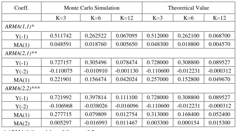
According to the previous derivation, AR model is stable and its lag order remains unchanged. And it is not difficult to find that the coefficients of B are the k times power that of the operator L. We illustrate three models respectively for simulation, that is, ARMA(1,1), ARMA(2,1) and ARMA(2,2), which verifies the theory of model derivation above, and we also find some special regularities that could not be observed in theory.

Table 2. Monte Carlo Simulation (Stock y).

Coeff. Monte Carlo Simulation Theoretical Value

K=3 K=6 K=12 K=3 K=6 K=12

ARMA(1,1)*

Y(-1) 0.511742 0.262522 0.067095 0.512000 0.262100 0.068700

MA(1) 0.048591 0.018760 0.005650 0.048300 0.018800 0.004570

ARMA(2,1)**

Y(-1) 0.727157 0.305496 0.078474 0.728000 0.308800 0.089527

Y(-2) -0.110075 -0.010910 -0.001130 -0.110600 -0.012231 -0.000312

MA(1) 0.221901 0.156474 0.042024 0.257000 0.152800 0.049670

ARMA(2,2)***

Y(-1) 0.721992 0.397814 0.111100 0.728000 0.308800 0.089527

Y(-2) -0.106968 -0.038026 -0.016096 -0.110600 -0.012231 -0.000312

MA(1) 0.277715 0.079809 0.012754 0.313000 0.168400 0.052400

MA(2) 0.005297 -0.016993 0.011467 0.003300 0.000154 0.015300

* ARMA(1,1) model:y_t=0.8y_t-1+u_t+0.2u_t-1

** ARMA(2,1) model: yt=1.4yt-1-0.48yt-2+ut+0.2ut-1

*** ARMA(2,2) model: y_t=1.4y_t-1-0.48y_t-2+u_t+0.2u_t-1+0.1u_t-2

be infinite, coefficients of AR lagging part are all tend to zero, which means they all lose explanation to y. Only y_T* remains, the whole model confirms to AR(1) form.

Coefficients of MA model are based on θ and δ, we use control variable method to explore whether there is a relationship between β and δ. Since the MA part is solved by equation systems, hence we are not capable of expressing it in concrete mathematical form, so we fail to infer the explicit trend relation between δ and β.

It is apparent that β will influence the accuracy of AR model estimation, which reminds us that δ may account for the coefficient bias between theory and simulation. Note that when k grows, coefficients may be too small to be significant, such as case k=12 showed in the table.

Summary

The paper has considered temporal aggregation of ARMA model, including model derivation and regularity results, and applied Monte Carlo simulation to verify the theory. We showed that temporal aggregation transfer model of ARMA is accurate as long as k is appropriate, but there are times that bias will emerge and researchers have to pay attention to. With this method, unexpected shocks or fluctuations can be timely integrated into the forecasting model for better prediction.

Acknowledgements

We are grateful to our teacher Zengmin Wang for inspiring our thoughts and strongly supporting us along the whole research process. Besides, this research is financially supported by the Research Innovation Fund for College Students of Beijing University of Posts and Telecommunications.

References

[1] Amemiya T, Wu R Y. The effect of aggregation on prediction in the autoregressive model[J]. Journal of the American Statistical Association, 1972, 67(339): 628-632.

[2] Brewer K R W. Some consequences of temporal aggregation and systematic sampling for ARMA and ARMAX models[J]. Journal of Econometrics, 1973, 1(2): 133-154.

[3] Marcellino M. Some Consequences of Temporal Aggregation in Empirical Analysis[J]. Journal of Business & Economic Statistics, 1999, 17(1):129-136.

[4] Rossana R J, Seater J J. Temporal aggregation and economic time series[J]. Journal of Business & Economic Statistics, 1995, 13(4): 441-451.

[5] Silvestrini A, Veredas D. Temporal aggregation of univariate linear time series models[M]. CORE, 2005.

[6] Silvestrini A, Veredas D. Temporal aggregation of univariate and multivariate time series models: a survey[J]. Journal of Economic Surveys, 2008, 22(3): 458-497.

[7] Wei, William W S. Some Consequences of Temporal Aggregation in Seasonal Time Series Models[J]. Nber Chapters, 1978.